Article

Evaluation of Strategies to Reducing Traction Energy Consumption of Metro Systems Using an Optimal Train Control Simulation Model

State Key Laboratory of Rail Traffic Control and Safety, Beijing Jiaotong University, No.3, Shangyuncun, Haidian District, Beijing 100044, China
*
Author to whom correspondence should be addressed.
Energies 2016, 9(2), 105; https://doi.org/10.3390/en9020105
Submission received: 5 December 2015 / Revised: 20 January 2016 / Accepted: 22 January 2016 / Published: 12 February 2016

Abstract

:
Increasing attention is being paid to the energy efficiency in metro systems to reduce the operational cost and to advocate the sustainability of railway systems. Classical research has studied the energy-efficient operational strategy and the energy-efficient system design separately to reduce the traction energy consumption. This paper aims to combine the operational strategies and the system design by analyzing how the infrastructure and vehicle parameters of metro systems influence the operational traction energy consumption. Firstly, a solution approach to the optimal train control model is introduced, which is used to design the Optimal Train Control Simulator(OTCS). Then, based on the OTCS, the performance of some important energy-efficient system design strategies is investigated to reduce the trains’ traction energy consumption, including reduction of the train mass, improvement of the kinematic resistance, the design of the energy-saving gradient, increasing the maximum traction and braking forces, introducing regenerative braking and timetable optimization. As for these energy-efficient strategies, the performances are finally evaluated using the OTCS with the practical operational data of the Beijing Yizhuang metro line. The proposed approach gives an example to quantitatively analyze the energy reduction of different strategies in the system design procedure, which may help the decision makers to have an overview of the energy-efficient performances and then to make decisions by balancing the costs and the benefits.

1. Introduction

Metro systems aim to provide frequent, safe and comfortable journeys to a large number of passengers in a short period of time, which make them become an important part of public transportation to relieve traffic congestion. In addition, metro systems can transport more passengers with less energy consumption and, thus, are regarded as a green transportation mode when compared to buses and private car services. However, due to the large-scale operations of metro systems (especially in big cities) and high-frequency services, a great amount of energy is consumed for the daily operation. For example, in Beijing metro systems, there are 18 operating lines, and the passengers can on average reach 10 million per day, which could increase to 11.5 million for peak periods. The corresponding annual energy consumption is over 500 MWh. Hence, improving the energy efficiency of metro systems will be of great interest for the operation company to reduce the energy consumption, as well as the operational cost. Furthermore, according to the investigation in the Railenergy project [
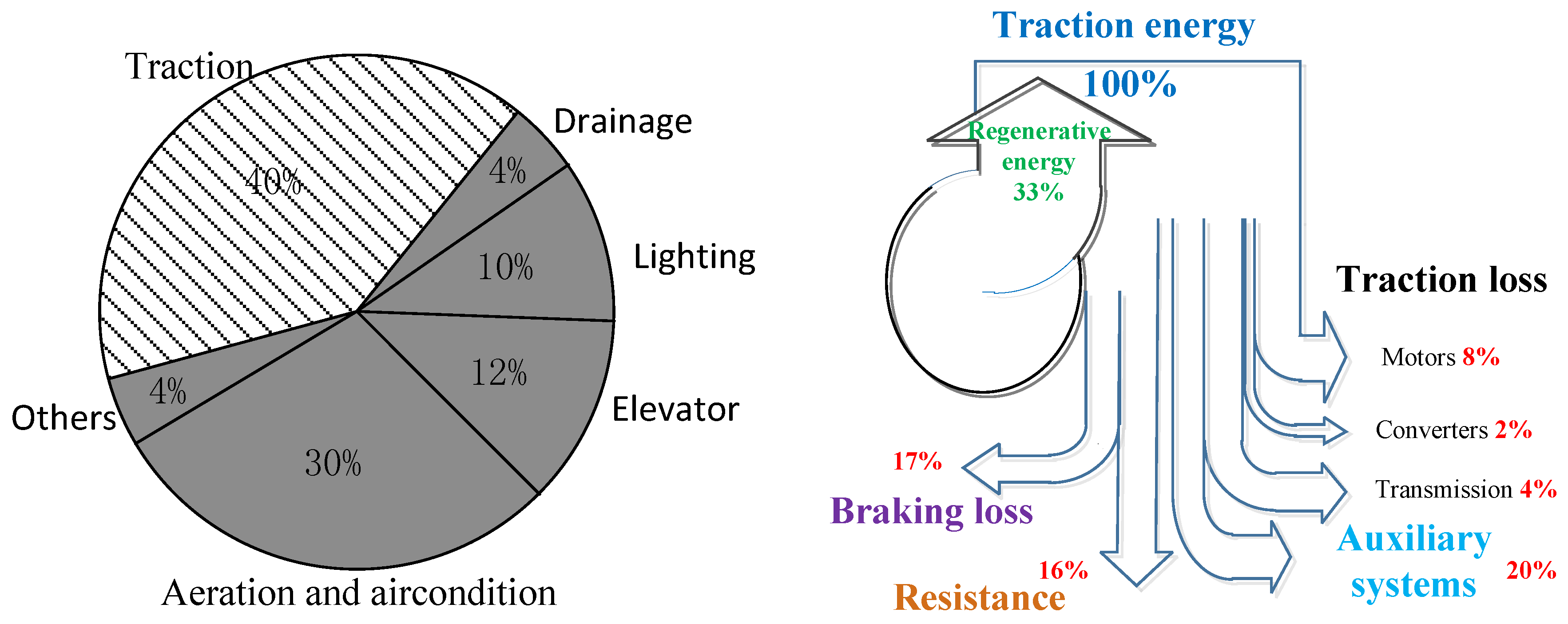
1], the energy consumption in metro systems is mainly consumed in traction, aeration, air condition, elevator, lighting and drainage (see Figure 1), among which the traction energy plays the most important role. This implies that reducing the traction energy has a great potential in improving the energy efficiency of metro systems, which will be studied in this paper consequently.
Figure 1. Energy consumption in metro systems.
Energies 09 00105 g001
As shown in 
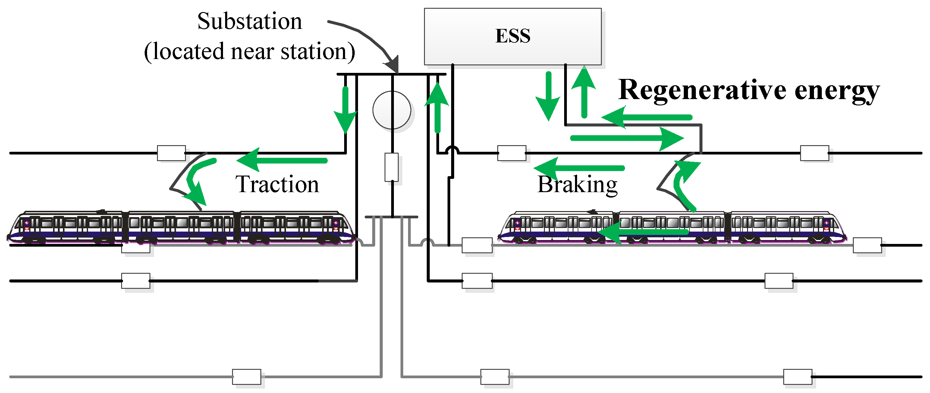
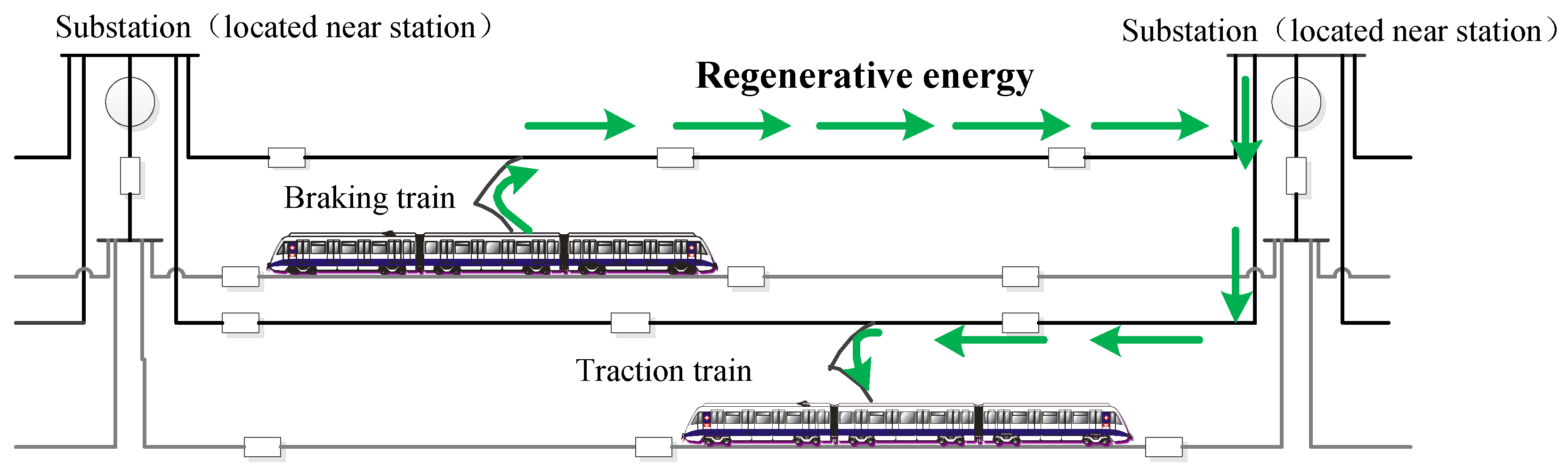
Figure 1, the traction energy absorbed from the power supply system is mainly consumed at the auxiliary system, overcoming the resistance, traction loss and the braking loss. For most metro systems, the train’s kinetic energy can be converted back to electric energy when trains apply regenerative braking. This part of regenerative braking energy can be reused by itself, stored in on-board energy storage systems or be transmitted backwards to the overhead catenary or the third rail and utilized by other trains, i.e., the regenerative energy could be reused in the systems. Hence, the research on reducing the train traction energy consists of two aspects: cutting down the losses and increasing the reused regenerative energy.
From the view of system engineering, the energy-efficient strategies can also be classified into operational strategies and energy-efficient system design. Operational strategies aim to optimize the utilization of the traction energy with the given infrastructure and vehicle conditions, e.g., energy-efficient driving strategy and timetable optimization. For a given interval, many driving strategies are feasible with the fixed trip time, among which the energy-efficient driving strategy consumes the minimum energy. Many literature works studied the optimal train control strategies to minimize the mechanical traction energy [2,3]. The constraints in the optimal train control model include the trip time, trip distance, maximum traction force, the maximum braking force and speed limit. Additionally, the optimization problem can be solved by analytic methods [4,5], numerical methods [6,7] and searching algorithms [8,9]. Differing from the works mentioned above, this paper gives a detailed analysis on how the factors in the optimal train control model influence the trains’ energy consumption and presents some possible energy-efficient strategies for metro systems. Recently, theoretical studies have been directed towards the problem of designing an energy-efficient timetable to save energy [6,10]. Albrecht [10] proposed a dynamic programming approach to find the energy-efficient trip times based on the solution to the optimal train control problem. Su [6] used an iterative algorithm to obtain the driving strategy for the entire route, which integrated the driving strategy optimization and the distribution of the trip time. Scheepmaker [11] incorporated energy-efficient train operation into the railway timetable by distributing the time supplements into segments, and the robustness of the generated timetable was analyzed. Similar studies can be found in [12,13]. Su [14] proposed a cooperative train control model to efficiently use the regenerative energy by adjusting the departure time of the accelerating train. Gong [15] proposed an energy-efficient operation methodology for metro lines, including timetable optimization and the driving strategy optimization. The proposed approach in [15] can adjust the dwell time of trains for better utilization of the regenerative energy.
Energy-efficient system design integrates the efficient strategies into the design process, such that the operational energy consumption could be reduced. To some extent, the energy-efficient system design is of greater significance. Some researchers have studied smart infrastructure and vehicle design methods to improve the efficiency of the metro systems, including the mass reduction, the energy-efficient slopes, the installation of energy storage and the improvement of aerodynamics. Carruthers [16] analyzed the influence of the material selection on the train mass and proposed that 7% of the savings in energy can be achieved with a 10% reduction in the train mass. Similar studies were done by Rochard [17]. Walter [18] gave an overview of the various possibilities of increased energy efficiency in electric railway systems, and highly reliable energy storage was focused on to save energy and operation cost in the paper. Wang [19] and Xia [20] studied the optimization on the location and size of the energy storage systems in metro lines, acting as a compromise between satisfying better energy savings, voltage profile and lower installation cost.
The contribution of this paper is to create a connection between the operational strategies and the system design strategies. The relative energy-efficient strategies are analyzed, and the influence of the system design on the operational energy consumption can be quantitatively evaluated with the optimal train control solution. The simulation results can give the decision makers an overview of the energy-efficient performances with different strategies, which may help them to balance with the investment according to their practical experience and make the final decision from a short- or a long-term view.
The rest of this paper is organized as follows. In Section 2, the optimal train control model and the corresponding solution are presented. In Section 3, some energy-efficient strategies with the optimal train control model and the energy-efficient performances are evaluated with the practical data of the Beijing Yizhuang metro line. A short discussion and future work are included in Section 4.

2. Optimal Train Control Model

The optimal train control problem applies the optimal control theory to optimize the driving strategy between successive stations, such that the mechanical traction energy is minimized [3,21].
m i n E ( T ) = 0 T k t ( t ) v ( t ) F ( v ( t ) ) d t .
E, T and v are the energy consumption, trip time and train speed, respectively. F denotes the available maximum traction force, and k t is the relative traction force, i.e., the ratio between the applied traction force and the maximum traction force. The mass-point model of the train is widely used to describe the train movement as the following equations:
m d v ( t ) d t = k t F ( v ( t ) ) k b B ( v ( t ) ) g ( s ) r ( v ) , d s d t = v ,
where B and k b denote the available maximum braking force and the relative braking force. g is the gradient and curve resistance. r is the running resistance, which includes the friction and air resistance. Generally, trains will not apply the traction and braking forces at the same time. Hence,
k t * k b = 0 .
The boundary conditions and the constraint on the speed limit are:
v ( 0 ) = v ( T ) = 0 , v V ¯
In addition, the trip distance constraint should be satisfied,
L = 0 T v ( t ) d t
Additionally, the constraints on the relative traction and braking force are shown as follows.
k t [ 0 , 1 ] , k b [ 0 , 1 ]
The optimal train control model is concluded as Equations (1) to (6). By using the the Pontryagin maximum principle, the optimal driving strategies are proven to consist of maximum acceleration, cruising with partial power, cruising with partial braking, coasting and maximum braking [3,5]. The previous works [6,7] have proposed a numerical algorithm to calculate the energy-efficient driving strategy, which includes the control sequences and the corresponding switching points. The proposed algorithm will firstly present an iterative algorithm to calculate the driving strategy for one section. Then, the solution is extended to solve the driving strategy of multiple sections by distributing the energy units to sections.

2.1. Calculation of the Driving Strategy for One Section

It is noted that the minimum energy consumption is uniquely determined by the trip time and vice versa. Hence, the energy-efficient driving strategy can be calculated with either the known trip time or the known energy consumption. For a section (section in the algorithm is defined as a small part of the trip with a constant gradient and speed limit), the driving strategies of each section will be maximum acceleration (MA), cruising (CR), coasting (CO) and maximum braking (MB) [22]. With the given energy consumption, we can firstly generate the speed sequences for the MA phase. The CR speed sequences will be calculated with the remaining energy when the train speed has reached the speed limit. The speed sequences of the rest of the journey will be covered by the CO and MB phases. The details for obtaining the speed sequences of a given section are described in Algorithm 1.
Algorithm 1: calculation of the energy-efficient driving strategy for a given section.
Step 1:
Initialize the initial speed v 0 j and the energy consumption Ej for section j;
Step 2:
Divide the section into nj pieces, such that the distance of each piece is Δx;
Step 3:
Generate the speed sequences for the MA phase;
v i j = v 0 j , while Ej > 0, v i j < V, do
v i + 1 j 2 v i j 2 = 2 Δ x ( F ( v i j ) / m r ( v i j ) / m g ( x i ) / m ) ,
E = E F ( v i j ) Δ x ;
Step 4:
If the speed v i j has reached the speed limit, then partial braking or partial power is applied to keep cruising, and the speed sequences are calculated as v i + 1 j = v i j ;
Step 5:
Generate the speed sequences for CO phase as, v i + 1 j 2 v i j 2 = 2 Δ x ( r ( v i j ) / m g ( x i ) / m ) ;
Step 6:
If the MB phase exists, we calculate the braking speed sequences { v i j } as, v k j = v t j , v i + 1 j 2 v i j 2 = 2 Δ x ( B ( v k j ) / m r ( v k j ) / m g ( x K ) / m ) , and then, let v i j = min ( v k j , v t j ) ;
Step 7:
Return the optimal speed sequences v i j and the trip time of this section T j = i = 0 n j Δ x v i j .
Δ x is a small distance unit, which is assumed to be 1 m in the algorithm.

2.2. Calculation of the Driving Strategy for Multiple Sections

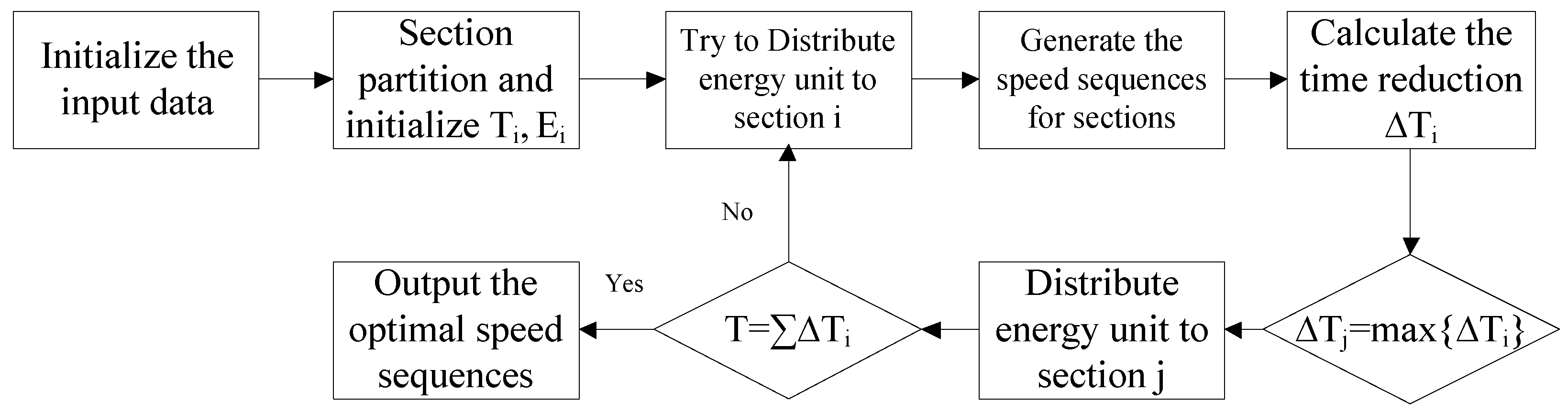
For dealing with variable gradients and speed limits, the trip is divided into several sections, such that each section has the constant gradient and speed limit. The speed sequence of each section can be generated by Algorithm 1. Then, based on a primary solution, the energy unit (a small amount of energy, which is assumed to be 0.05 kW·h in this algorithm) will be attempted to distribute to each section for achieving the corresponding time reductions. After a comparison among these time reductions, the energy unit will be finally assigned to the section that can achieve the maximum time reduction. This distribution process will be repeated to shorten the primary trip time until the practical trip time is delivered, after which the driving strategy and the speed profile will be obtained. The flow chart of the algorithm is described in Figure 2 [6,7,23].
Figure 2. The flow chart for calculating the energy-efficient driving strategy of multiple sections.
Energies 09 00105 g002
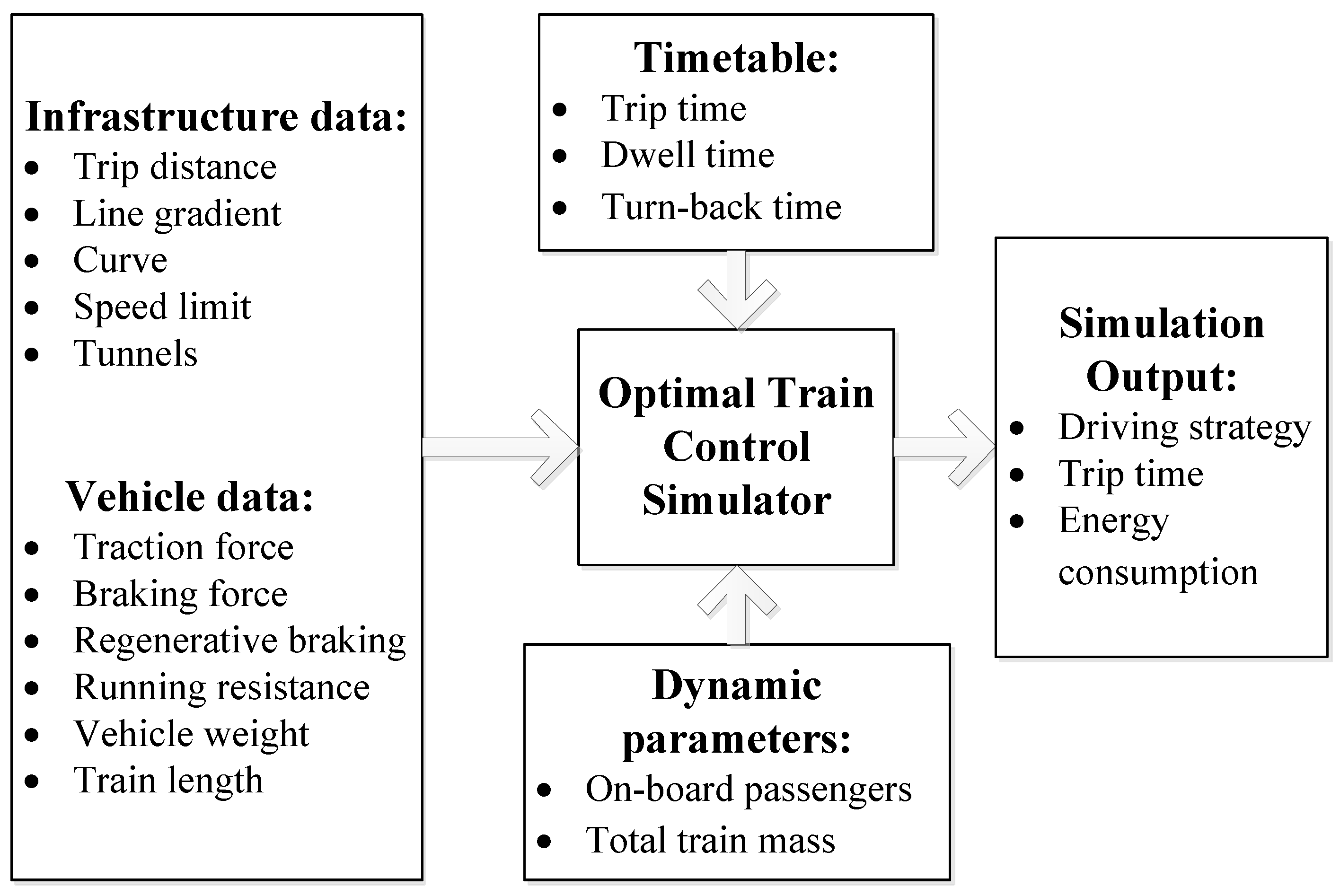
The algorithm is used to design an Optimal Train Control Simulator (OTCS). The trip distance, trip time, gradient, resistance, traction and braking characteristics and train mass are the inputs. The energy-efficient train control strategies and the corresponding energy consumptions are the outputs (see Figure 3). When the train stops at stations are taken as a speed limit of 0 km/h, the OTCS can also be used to calculate the energy-efficient driving strategy for multiple interstations, as well as the trip time at each interstation.
Figure 3. The flow chart of the OTCS.
Energies 09 00105 g003

3. Energy-Efficient Strategies

To advocate a sustainable rail transportation, many measures have been taken to save energy. According to the optimal train control model, the possible factors that influence the traction energy consumption are the trip time, the gradient, the running resistance, the maximum traction and braking forces, the regenerative braking and the train mass according to the OTCS. In the following subsections, the influence of these factors on the traction energy consumption is analyzed separately based on OTCS, from which effective solutions to saving energy are presented. The simulations are based on the practical data of the Beijing Yizhuang line.

3.1. Data Preparation

3.1.1. Vehicle Data

The running resistance can be calculated [24] by:
r ( v ) = 0.005 × v 2 + 0.23 × v + 2.965 kN
The maximum traction force is given as follows.
F ( v ) = 310 kN , v 10 m / s F ( v ) = 310 ( v 10 ) * 10 kN , 10 < v 22.2 m / s
The maximum electrical braking force is calculated by:
B ( v ) = 260 kN , v 15 m / s B ( v ) = 260 ( v 15 ) * 18 kN , v > 15 m / s
Note that the practical braking force is the combination of the mechanical braking and electrical braking forces. The electrical braking force is small when trains run with a high speed, and the mechanical braking can supply the needed braking force. Hence, the braking force can be taken as a constant in metro systems. In the following simulations, the maximum braking force is assumed to be 260 kN if there is no specific explanation. The electrical braking force is used to calculate the regenerative braking energy.
The vehicles on the Beijing Yizhuang line consist of six car units, three of which are traction units. The mass of each traction unit and non-traction unit is about 35 t and 31 t, respectively. The net total train mass is about 198 t. The normal train capacity is 1500, but the number of on-board passengers can reach 2000 in peak hours. The general, train mass in the simulation is assumed to be 250 t according to the operational experience, and the maximum train mass is 320 t. Other vehicle information is given in Table 1.
Table 1. Vehicle information.
ParametersValueParametersValue
Normal train mass286 tGearing Efficiency0.93
Over-load train mass311 tMaximum speed80 km/h
AC motor power180 kWMaximum acceleration1.2 m/s 2
Pantograph impedance0.015 ΩMaximum deceleration−1 m/s 2
Inverter efficiency0.97Equivalent internal resistance0.07 Ω

3.1.2. Infrastructure Data and Timetable

The infrastructure data of the Beijing Yizhuang line, including the altitude of the line and the speed limit for each position, is shown in Figure 4. Stations (used for trains’ stopping and passengers’ alighting and boarding) from Jiugong to Jinghailu are above the ground, and the other six stations are underground. Hence, there are two steep slopes near Jiugong and Jinghailu station. The gradient acceleration rate of a section can be obtained with the altitude difference in Figure 4. Note that the gradient for trains running from Yizhuang to Songjiazhuang and the gradient for trains running from Songjiazhuang to Yizhuang are symmetric. In addition, there is normally a speed limit of 54 km/h near stations, and the corresponding distance is about 150 m. The speed limit of the other sections is generally 80 km/h. The speed limit of all sections is the same for the trains of two directions.
Figure 4. Gradient and speed limits of the Beijing Yizhuang line.
Energies 09 00105 g004
The current simplified timetable of the Yizhuang line is shown in Table 2. Note that the turn-back times at Songjiazhuang and Yizhuang are 3 min in the timetable.
Table 2. Operation situation of the Yizhuang metro line.
SegmentDistance
(m)
Dwell Times
(s)
Trip Times
(Up-Bound) (s)
Trip Times
(Down-Bound) (s)
Songjiazhuang-Xiaocun263130190195
Xiaocun-Xiaohongmen127530108105
Xiaohongmen-Jiugong236630157157
Jiugong-Yizhuangqiao198235135135
Yizhuangqiao-Wenhuayuan993309090
Wenhuayuan-Wanyuan153830114111
Wanyuan-Rongjing128030103101
Rongjing-Rongchang135430104103
Rongchang-Tongjinan233830164162
Tongjinan-Jinghai226530150158
Jinghai-Ciqunan208630140141
Ciqunan-Ciqu128635102100
Ciqu-Yizhuang133445105110
Specifically, some simulation in the following sections is based on the interstation between the Jiugong and Yizhuangqiao station. Hence, the detailed gradient and speed limit for this journey is given in Table 3.
Table 3. Infrastructure data between Jiugong and Yizhuangqiao station. The negative gradient in the second column means downhill gradients.
Position (m)Gradient (‰)Speed Limit (km/h)Position (m)Gradient (‰)Speed Limit (km/h)
0–1300541029–1115080
130–4660801115–1405−280
466–543−4801405–1768−380
543–700−6801768–1802−280
700–7610801802–1840−180
761–8517801840–1975054
851–10291280---

3.1.3. Substation

The Yizhuang line contains 12 substations (used for supplying power to trains), which are located at each station, except the second station (Ciqu) and eighth station (Wanyuan) (see Table 4). Some other substation-related information is given in Table 5.
Table 4. Location of substations.
Substation123456789101112
Location02.624.716.979.3110.6613.4814.4716.4618.8220.1022.73
Table 5. Substation-related information.
ParametersValueParametersValue
Number of Substations12Auxiliary Power45 kW
substation voltage with no load850 Vmaximum tractive power3680 kW
substation inner resistance0.02 ΩContact line impedance0.007 Ω/km
over-voltage limitation930 VRail impedance0.009 Ω/km

3.2. Trip Time

In the left figure of Figure 5, the relation between the trip time and energy consumption is illustrated. With the increase of the trip time, the energy consumption decreases. In practical operation, the dwell time for one station is constant on the Beijing Yizhuang line. The practical dwell time is sometimes shorter than the scheduled dwell time in off-peak hours, which always happens in metro systems. If the driver could close the door immediately after passengers’ boarding and alighting process, the trip time for the next interstation will be prolonged, and the energy consumption will be reduced effectively. By training the drivers, the invalid dwell time will be utilized in the next interstation, which makes better use of the timetable to save energy.
In addition, the function between the energy consumption and the trip time is convex, which means that it costs more energy to achieve the same time reduction when the trip time is shorter (see the left picture in Figure 5). For example, the energy consumption increases by 3.4 kWh when the trip time is reduced from 160 s to 150 s, compared to 4.8 kWh when the trip time is reduced from 150 s to 140 s.
Similarly, E-T functions of interstations are discrepant, and then, the energy consumptions for the same time reduction are different for different interstations (see the right picture in Figure 5), which can be used to optimally distribute the running time supplements among multiple interstations [7,11]. Taking the Yizhuang line as an example, the driving strategies for each interstation are firstly optimized with the OTCS. Compared to the practical operation, the energy reduction is 8.64% with the energy-efficient driving strategy. Next, the trip time and the driving strategy are optimized together with the OTCS, and the traction energy consumption of the new timetable is calculated. As shown in Table 6, the total traction energy consumption for multiple interstations can be reduced by 12.07%. This implies that the optimized timetable has a good potential for energy savings.
Figure 5. Influences of the trip time on the traction energy consumption.
Energies 09 00105 g005
Table 6. Comparison of energy consumption between the energy-efficient driving strategy and integrated timetable optimization; the unit of the energy consumption is kW·h.
InterstationPractical Trip TimePractical Energy ConsumptionEnergy with Optimized Driving StrategyOptimal Trip TimeEnergy with Integrated Approach
Songjiazhuang-Xiaocun19029.87621.056179.328.563
Xiaocun-Xiaohongmen10810.0049.568108.78.996
Xiaohongmen-Jiugong15720.30219.680153.621.652
Jiugong-Yizhuangqiao13520.51519.932134.620.303
Yizhuangqiao-Wenhuayuan9015.97315.02592.112.011
Wenhuayuan-Wanyuan11414.98014.051116.911.547
Wanyuan-Rongjing1039.1568.903105.47.922
Rongjing-Rongchang10413.06812.293108.410.015
Rongchang-Tongjinan16411.32210.446152.813.779
Tongjinan-Jinghai15021.71120.047149.220.806
Jinghai-Ciqunan14027.62925.684144.120.174
Ciqunan-Ciqu10222.94421.399106.418.090
Ciqu-Yizhuang10515.77015.015110.611.237
Total1662233.250213.0991662205.095
Energy savings (%)--8.64-12.07
Hence, two techniques are concluded with respect to the trip time:
  • Increase the trip time by reducing the invalid dwell time;
  • Timetable optimization.

3.3. Train Mass

In this subsection, the influence of the train mass on the traction energy consumption is studied, which is shown in Table 7. In this case, the running time is fixed (145 s), and the corresponding energy consumptions are calculated with different train masses based on the OTCS. Obviously, the heavier the train is, the more energy consumption it will consume during the trip, since more traction force or a longer duration of traction will be applied to achieve the same train speed for a heavier train. The results illustrate that the energy consumption will show a great increase from 16.8 kWh for 200 t to 31.2 kWh for 300 t. In other words, the energy consumption is nearly doubled when the train mass increases by 50%. Hence, the mass reduction is proposed as one of the important strategies to save energy, not only for metro systems, but also for main line railway systems.
Table 7. Energy consumptions with different train masses.
Train Mass (t)Energy Consumption (kW·h)Train Mass (t)Energy Consumption (kW·h)Train Mass (t)Energy Consumption (kW·h)
20016.823520.827025.6
20517.224021.227526.4
21017.624522.028027.2
21518.425022.828528.0
22018.825523.229029.2
22519.226024.029530.0
23020.026524.830031.2
Important measures to reduce the train mass are concluded as follows [16,17]:
  • Selection of light material, e.g., aluminum alloy;
  • Development of new vehicle structure;
  • Optimization of component design.

3.4. Gradient

In this subsection, we study the influence of the gradient on the traction energy consumption. Three typical sections are chosen as examples in the case studies, i.e., the starting section from 130–466 m, the middle section from 761–851 m and the caudal section from 1840–1975 m. The gradients of these three sections change from −4‰–11‰, from 1‰–15‰ and from −5‰–10‰, respectively. The traction energy consumptions of the interstation from Jiugong to Yizhuangqiao station are calculated with each gradient, which is shown in Table 8. The results show that more energy will be consumed with the increase of the gradient for the starting section. The reason can be explained as that more traction force or a longer duration of the traction force must be applied to deliver the required trip time for a steeper uphill climb. On the contrary, the traction energy consumption will decrease with an increasing gradient of the caudal section. Since a higher braking rate can be obtained with a steeper uphill climb and the train needs less time to come to a standstill, so, in order to deliver the same trip time with a higher braking rate, trains can accelerate to a lower speed, which therefore costs less energy. In addition, more energy is needed when the gradient of the middle section is greater. It is obviously that the train will consume more energy to overcome the gradient resistance. It is also concluded that the longer the section distance is, the greater influence it will have on the traction energy consumption. Specifically, the distance of the starting section is 336 m, much longer than 90 m and 135 m in the middle and caudal sections. Additionally, the energy consumption increases by about 0.8 kWh when the gradient of the starting section gains 2‰ uphill, compared to only 0.1 kWh for the middle and caudal sections.
Table 8. Energy consumptions for different gradients.
SectionParametersValue
1G (‰)−4−3−2−10123
Energy (kWh)21.021.421.822.222.623.023.323.7
G(‰)4567891011
Energy (kWh)24.124.524.925.225.626.026.426.8
2G (‰)12345678
Energy (kWh)21.821.821.921.922.022.022.122.1
G (‰)9101112131415-
Energy (kWh)22.222.322.422.522.622.722.8-
3G (‰)−5−4−3−2−1012
Energy (kWh)22.822.822.722.722.722.622.622.5
G (‰)345678910
Energy (kWh)22.522.422.322.222.222.122.122.0
Energy-efficient train operation should couple with a larger acceleration rate in the beginning, less gradient resistance in the middle section and a larger braking rate at the end of the trip [25]. Generally, the vertical alignment is always designed to be downhill, slightly downhill and uphill in shape to save the operational traction energy (see Figure 6). In addition, when we consider the trains in both directions, the downhill gradient of the middle section in one direction implies uphill in the other direction. Trains need to apply traction to achieve the gravitational potential energy for the uphill gradient; while the gravitational potential energy can normally be used by trains running in the other direction. A qualitative conclusion is drawn that the gradient in the middle section has little influence on the total traction energy consumption of the operational systems.
Figure 6. Design of energy-saving slopes.
Energies 09 00105 g006
Although the slopes near stations could contribute to saving energy, the length of the slopes should be paid attention to for a high efficiency. Generally, there is no doubt that trains should overcome the gradient resistance for a steep uphill slope. However, the gravitational potential energy may not be used for trains in the reverse direction if the length of the gradient is too long. As shown in Figure 7, the red, black, blue and green curves denote the emergence braking speed, train speed, traction or braking force and the gradient. The data are from the practical operations of trains running between Yizhuang and Ciqu stations of the Yizhuang line. There is a steep slope near Yizhuang station according to the infrastructure data. For trains running from Yizhuang to Ciqu, the downhill slope could help the trains to achieve a high speed with a shorter time until the train reaches the target speed. Then, the train has to apply braking to slow down the speed, such that it will not trigger the emergency braking. As a result, the gravitational potential energy is wasted in some sense.
The proper length for the energy-efficient slop design will depend on the train length, traction and braking characteristics and the maximum speed train speed. As shown in Table 9, the acceleration distance will vary with different acceleration rates and the maximum train speed. Normally, the platform is designed on a flat gradient, and the energy-efficient slopes should be considered according to the acceleration distance. Taking the Yizhuang line as an example, the maximum train speed is 80 km/h with an average acceleration of 0.60 m/s 2 . The acceleration distance is about 407 m. As shown in the right picture in Figure 6, the length of the energy-efficient gradient should be about 330 m, except the flat gradient in the platform.
Figure 7. Influence of the gradient length on the energy consumption. (a) Driving strategy from Yizhang to Ciqu station; (b) driving strategy from Ciqu to Yizhang station.
Energies 09 00105 g007
Table 9. Length of the energy-efficient slopes with different train types.
ParametersValue
Maximum Speed (km/h)80859095100105110115120
Average acceleration rate (m/s 2 )0.600.570.550.520.500.480.470.460.45
Acceleration time (s)374145.550.755.660.863.667.974.1
Acceleration distance (m)40748856866976988497210851234
Length of trains (m)140140145148140142160162160
Length of the slope (m)3304104905906908008709801120
Important measures of the energy-efficient gradient design are concluded as follows:
  • Increase the gradient near stations;
  • Proper length of the gradient.

3.5. Maximum Acceleration and Braking

In this subsection, we calculate the traction energy consumptions with different maximum traction and braking forces with the OTCS. The results are shown in Table 10, which reveals that the traction energy consumption presents a gentle decrease with the increase of the maximum traction and braking forces. Definitely, the traction energy consumption is 23.70 kWh when the maximum traction force is 285 kN, which decrease by 7.0% to 22.06 kWh when the maximum traction force is 360 kN. Additionally, the traction energy consumptions are 23.90 kWh, 23.50 kWh, 22.50 kWh and 21.90 kWh, respectively, with the corresponding maximum braking forces as 255 kN, 270 kN, 305 kN and 345 kN. The energy consumption increases by 8.4% with the maximum braking force rising by 50%.
Table 10. Traction energy-saving performance with different maximum traction and braking forces.
ParametersValue
Maximum traction force (kN)285290295300305310315320
Energy consumption (kWh)23.7023.5823.4623.3423.2323.1122.9922.88
Maximum traction force (kN)325330335340345350355360
Energy consumption (kWh)22.7522.6322.5122.4022.3022.2122.1322.06
Maximum braking force (kN)255260265270275280285290
Energy consumption (kWh)23.9023.7723.6423.5023.3223.1522.9922.83
Maximum braking force (kN)295305310320330335340345
Energy consumption (kWh)22.6622.5022.4122.3022.1922.0921.9921.90
The reasons are explained as follows. By comparing the Speed Profiles 1 and 2 in Figure 8, the train should accelerate to a higher speed with a low acceleration rate for delivering the same trip time, which will consume more energy. By making a comparison between the Speed Profiles 2 and 3, we can obtain that the train with a higher braking rate can come to a stop more quickly, and then a lower speed is needed during the trip, which could reduce the traction energy consumption. In conclusion, vehicles with larger traction and braking forces will be more energy efficient.
Figure 8. Driving strategy with different maximum traction and braking forces.
Energies 09 00105 g008

3.6. Regenerative Braking

Many modern metro vehicles are capable of converting kinetic energy into electrical energy when trains apply electrical braking, which is known as regenerative braking. According to [1], approximately 30% of the traction energy from the braking train can be recovered and then reused in the systems. More importantly, the characteristic of the train operations in metro systems is that the maximum acceleration and electrical braking regimes frequently happen, which provides a good opportunity for trains to utilize the regenerative energy. Efficient utilization of the regenerative energy could make a great difference in reducing the energy consumption of metro systems. The recovered regenerative energy can be firstly used by the on-board systems, such as lights, carborne signaling systems and air conditioning. The rest of energy will be fed back to the power network, such that it can be used by the other accelerating trains. The energy could also be stored in the energy storage systems (ESSs) and then be reused by trains. Hence, the utilization of regenerative braking energy can be classified into two ways, i.e., immediate energy exchange between trains and energy exchange between trains through ESSs.
For the storage of the regenerative energy, ESSs (such as super-capacitor, batteries, flywheels and superconducting magnetic energy storage [26]) should be installed. According to the installation position, the ESSs can be divided into two types, i.e., ESSs on the trains or ESSs along the track side. The on-board ESSs, e.g., super-capacitor and batteries, are installed on trains, and the stored regenerative energy can only be used by the train itself. The advantage is that the efficiency of the reused regenerative energy is high, since this energy can be duratively and effectively utilized with less line losses. However, the installation of the on-board ESSs will greatly increase the train mass and will require a large space, so it is seldom used in practice nowadays. The wayside ESSs can store the generated regenerated energy when nearby trains are applying regenerative braking. Then, the stored energy can be reused by the passing trains when they need it (see Figure 9). The application of the wayside ESSs requires an electrical controller to distinguish the driving strategy of the nearby trains by detecting the voltage of the power line [27]. Trains in rail and rapid transit systems are usually braking near stations, and thus, the ESSs are normally installed near stations to increase the recovery efficiency. Compared to the on-board ESSs, one of the advantages for the application of the wayside ESSs is that they can recover regenerative energy from multiple braking trains at the same time, and their installation has little influence the operation and maintenance. However, wayside ESSs are usually less efficient due to the transmission losses on the power line [28,29]. According to experimental results [30,31,32], the rate of energy reduction with ESSs ranges from 12%–20% for different lines.
Figure 9. Energy exchange between trains through energy storage systems (ESSs).
Energies 09 00105 g009
Immediate energy exchange between trains could achieve good utilization of the regenerative energy without installing other equipment (see Figure 10). However, the immediate energy exchange between trains needs cooperative operation between the braking and traction trains. Firstly, if there are no other traction trains when trains are braking, the regenerative energy will increase the voltage of the grid to a high level until the tolerative voltage limit is reached. Then, the following regenerative energy will be wasted at the braking resistance to protect the power network. Secondly, the distance between the traction and braking trains should be short to achieve a high efficiency. Furthermore, the driving strategy of the cooperative trains should be applying traction and braking at the same time. In conclusion, the traction and braking trains should be matched in the time, space and driving strategy. The trip distance of metro systems is short, and the traction and braking processes usually happen near stations. As a result, a good cooperation between trains can be achieved near stations by optimizing the train timetable.
In our previous work [14], a cooperative train control model has been studied, in which the regenerative energy is used better by adjusting the departure time. The simulation results show that the net energy consumption can be reduced by 11.34% for peak hours with combining the energy-efficient driving strategy and utilization of the regenerative energy.
Figure 10. Immediate energy exchange between trains by regenerative braking.
Energies 09 00105 g010

3.7. Running Resistance

The running resistance is another important factor that influences the traction energy consumption. As shown in the left figure in Figure 11, the energy consumption is 23.4 kWh for the current train operation from Jiugong station to Yizhuangqiao station, which will be reduced by 0.4 kWh with the resistance decreased by 10%. If the running resistance can be cut by 90%, the energy consumption with the same trip time will be 21.2 kWh, accounting for 90.6% of the current operation.
Figure 11. Influence of running resistance on the traction energy consumption.
Energies 09 00105 g011
In Figure 11, we simulate the traction energy consumption for different trip times when the running resistance is reduced by 20%. The average energy reduction is calculated to be 3%. The energy-saving performance of improving the running resistance is smaller than the other energy-efficient strategies; partially because the running resistance in metro systems is small and the energy consumption for overcoming the running resistance accounts for a smaller proportion. Note that there will be a significant difference for the scenarios in the high speed railway systems. The running resistance is the most important aspect that restricts the maximum train speed, and the traction energy consumption for overcoming the running resistance takes a large proportion in the total traction energy for high-speed railways. Furthermore, improving trains’ external geometry, trains’ surface roughness and the friction between trains and rail track can greatly contribute to the reduction of the resistance according to the technical report [33].
For metro systems, the running resistance is divided into basic running resistance and the additional resistance. The basic running resistance is generally calculated as:
r ( v ) = a * v 2 + b * v + c .
Normally, the coefficients a and b are related to the train mass and the interaction between tracks and train wheels. The coefficient c is related to the aerodynamics of the trains. The practical technologies include the following items.
  • Streamlining of head and tail;
  • Streamlining of train sides and underfloor areas;
  • Bogie fairings;
  • Aerodynamic optimization of pantographs;
  • Lubrication of wheels and tracks;
  • Mass reduction.
The additional resistance includes gradient resistance, tunnel resistance and curvature resistance. The gradient resistance has been analyzed in Section 3.4. The tunnel resistance can be generally obtained as:
r t u n n e l ( v ) = 0.00013 * L t r a i n ( N / k N ) ,
which is determined by the train length. When there is a speed limit at the tunnel, the tunnel resistance will be:
r t u n n e l ( v ) = V 2 * L t r a i n / 10 7 ( N / k N ) .
A lower speed limit and a shorter train length will contribute to reducing the tunnel resistance. In addition, the equation for calculating the curvature resistance is as follows.
r c u r v e = 600 / R ( N / k N ) .
If the length L c u r v e and the radius angle α of the curve are known, the equation can be transformed to be:
r c u r v e = 10.5 * α / L c u r v e , L c u r v e L t r a i n ; r c u r v e = 10.5 * α / L t r a i n , L c u r v e < L t r a i n ;
Based on the above analysis, the possible strategies include:
  • Enlarging the curve radius and the curve length;
  • Shortening the train length (without reducing the train capacity);
  • Reducing the speed limit at the tunnel.

3.8. Other Factors

In the subsections above, we have analyzed the possible factors that are related to the traction energy consumption based on the optimal train control model. Besides, there are also some other practical measures to save energy for metro systems. For example, the conversion losses will happen during the transmission, which may account for 10% of the total energy consumption. Hence, reducing the conversion losses at the inverters [34], traction motors and gears will make a significant difference on energy efficiency. Secondly, alternative concepts for autonomous traction, such as fuel cells [35] and hydrogen [36], might be needed in future railways. In addition, reducing energy consumption for comfort functions, improving the space utilization and increasing the load factor can also contribute to save the energy consumption of metro systems [33].

4. Conclusions and Future Research

The main contribution of this paper is to analyze how the factors in the optimal train control model influence the traction energy consumption based on the OTCS. A connection between the energy-efficient operational strategies and energy-efficient system design strategies has been built. Some energy-efficient design strategies, such as mass reduction, energy-efficient timetable, improving the air aerodynamics and friction, the good design of gradients, increasing the maximum traction and braking force and introducing regenerative braking, are concluded. These energy-efficient strategies are evaluated with the data of the Beijing Yizhuang metro line, as shown in Table 11. The simulation results illustrate that the energy reductions range from 1.5%–15% if appropriate improvement on one factor is made, which may be over 20% by integrating all of the energy-efficient strategies. Note that mass reduction, energy-efficient slopes and the improvement of vehicle traction and braking characteristics aim to achieve a fast acceleration process with the constraint of riding comfort. Except for saving energy, the installation of the ESSs on board may also increase the traction energy consumption by increasing the train mass. Hence, the integrated performance of all of the strategies is not simply the sum of all single strategies. The proposed research could give important implications to the operators, sponsors and engineers that the energy-efficient strategies should penetrate from the system design and operations procedures.
Table 11. Evaluation of different energy-efficient strategies.
FactorsStrategiesEnergy-Saving%
Trip timeTimetable optimization3.5
Train mass10% reduction7
GradientOptimized slopes distance2
Maximum traction forceIncrease by 10%3
Maximum braking forceIncrease by 5%1.5
Regenerative brakingInstallation ESSs15
Regenerative brakingTimetable optimization11
Running resistance15% reduction3
The application of the proposed energy-efficient strategies will be further studied in our future work. For example, the reduction of the train mass and the increasing of the maximum traction and braking forces may need new reformed vehicles. It is better to consider the design of the energy-efficient gradient in the system design period. When installing the ESSs, the costs and benefits should also be analyzed. This research will help the operators, sponsors and engineers to make the final decision.

Acknowledgments

This work was supported by the Beijing Laboratory of Urban Rail Transit, Beijing Key Laboratory of Urban Rail Transit Automation and Control, the Fundamental Research Funds for the Central Universities (No. 2014YJS029) and the projects funded by the Beijing Municipal Science and Technology Commission (No. D131100004113002 and No. D131100004013001) and the National Natural Science Foundation of China (No. 61503020).

Author Contributions

Tao Tang contributed to the conception of the study and provided the line and vehicle data. Shuai Su contributed significantly to analysis and manuscript preparation. Yihui Wang helped to perform the analysis with constructive discussions.

Conflicts of Interest

The authors declare no conflict of interest.

References

  1. Railenergy. Innovative Integrated Energy Efficiency Solutions for Railway Rolling Stock. Technical Report. 2006. Available online: http://www.uic.org/cdrom/2008/11_wcrr2008/pdf/R.3.4.3.1.pdf (accessed on 6 February 2016).
  2. Howlett, P.G. Optimal strategies for the control of a train. Automatica 1996, 32, 519–532. [Google Scholar] [CrossRef]
  3. Liu, R.; Golovitcher, I. Energy-efficient operation of rail vehicles. Transp. Res. Part A 2003, 37, 917–932. [Google Scholar] [CrossRef]
  4. Howlett, P.G.; Pudney, P.J.; Vu, X. Local energy minimization in optimal train control. Automatica 2009, 45, 2692–2698. [Google Scholar] [CrossRef]
  5. Khmelnitsky, E. On an optimal control problem of train operation. IEEE Trans. Autom. Control 2000, 45, 1257–1266. [Google Scholar] [CrossRef]
  6. Su, S.; Li, X.; Tang, T.; Gao, Z.Y. A subway train timetable optimization approach based on energy-efficient operation strategy. IEEE Trans. Intell. Transp. Syst. 2013, 14, 883–893. [Google Scholar] [CrossRef]
  7. Su, S.; Tang, T.; Li, X.; Gao, Z.Y. Optimization on multi-train operation in subway system. IEEE Trans. Intell. Transp. Syst. 2014, 15, 673–684. [Google Scholar]
  8. Ke, B.R.; Chen, M.C.; Lin, C.L. Block-layout design using max-min ant system for saving energy on mass rapid transit systems. IEEE Trans. Intell. Transp. Syst. 2009, 10, 226–235. [Google Scholar]
  9. Chang, C.; Sim, S. Optimising train movements through coast control using genetic algorithms. IEEE Electr. Power Appl. 2008, 144, 65–73. [Google Scholar] [CrossRef]
  10. Albrecht, T.; Oettich, S. A new integrated approach to dynamic schedule synchronization and energy-saving train control. Comput. Railw. VIII 2002, 61, 847–856. [Google Scholar]
  11. Scheepmaker, G.M.; Goverde, R.M.P. The interplay between energy-efficient train control and scheduled running time supplements. J. Rail Transp. Plan. Manag. 2015. [Google Scholar] [CrossRef]
  12. Zhao, N.; Roberts, C.; Hillmansen, S.; Western, P.; Chen, L.; Tian, Z.B.; Xin, T.Y.; Su, S. Train trajectory optimisation of ATO systems for metro lines. In Proceeding of the IEEE 17th International Conference on Intelligent Transportation Systems, Qingdao, China, 8–11 October 2014; pp. 1796–1801.
  13. Lin, W.S.; Sheu, J.W. Optimization of train regulation and energy usage of metro lines using an adaptive-optimal-control algorithm. IEEE Trans. Autom. Sci. Eng. 2011, 8, 855–864. [Google Scholar] [CrossRef]
  14. Su, S.; Tang, T.; Roberts, C. A cooperative train control model for energy-Saving. IEEE Trans. Intell. Transp. Syst. 2015. [Google Scholar] [CrossRef]
  15. Gong, C.; Zhang, S.W.; Zhang, F.; Jiang, J.G.; Wang, X.H. An integrated energy-Efficient operation methodology for metro systems based on a real case of Shanghai metro line one. Energies 2014, 7, 7305–7329. [Google Scholar] [CrossRef]
  16. Carruthers, J.J.; Calomfirescu, M.; Ghys, P.; Prockat, J. The application of a systematic approach to material selection for the lightweighting of metro vehicles. Proc. Mech. Eng. Part F J. Rail Rapid Transit 2009, 223, 427–437. [Google Scholar] [CrossRef]
  17. Rochard, B.P.; Schmid, F. Benefits of lower-mass trains for high speed rail operations. Proc. Inst. Civil Eng. Transp. 2004, 157, 51–64. [Google Scholar] [CrossRef]
  18. Walter, G. Technologies for increased energy efficiency in railway systems. Eur. Conf. Power Electron. Appl. 2005, 10, 1–10. [Google Scholar]
  19. Wang, B.; Yang, Z.P.; Lin, F.; Zhao, W. An improved genetic algorithm for optimal stationary energy storage system locating and sizing. Energies 2014, 7, 6434–6458. [Google Scholar] [CrossRef]
  20. Xia, H.; Chen, H.X.; Yang, Z.P.; Lin, F.; Wang, B. Optimal energy management, location and size for stationary energy storage system in a metro line based on genetic algorithm. Energies 2015, 8, 11618–11640. [Google Scholar] [CrossRef]
  21. Cheng, J.; Howlett, P. A note on the calculation of optimal strategies for the minimization of fuel consumption in the control of trains. IEEE Trans. Autom. Control 1993, 38, 1730–1734. [Google Scholar] [CrossRef]
  22. Hansen, I.; Pachl, J. Railway Timetable and Traffic; Eurailpress: Hamburg, Germany, 2008. [Google Scholar]
  23. Su, S.; Tang, T.; Chen, L.; Liu, B. Energy-efficient train control in urban rail transit systems. Proc. Inst. Mech. Eng. Part F J. Rail Rapid Transit 2015. [Google Scholar] [CrossRef]
  24. Kondo, M. Traction and Braking Performance of Beijing Subway Line; Techiqual Report; Dongyang Manufacturer of Motor: Tokyo, Japan, 2009. [Google Scholar]
  25. Xu, H.Z.; Cheng, G.Z.; Wu, C. Study on the design method of energy-saving slope in subway. Appl. Mech. Mater. 2012, 204–208, 1559–1564. [Google Scholar] [CrossRef]
  26. Gonzalez-Gil, A.; Palacin, R.; Batty, P. Sustainable urban rail systems: Strategies and technologies for optimal management of regenerative braking energy. Energy Conver. Manag. 2013, 75, 374–388. [Google Scholar] [CrossRef]
  27. Konishi, T.; Morimoto, H.; Aihara, T.; Tsutakawa, M. Fixed energy storage technology applied for DC electrified railway. IEEE Trans. Electr. Electron. Eng. 2010, 5, 270–277. [Google Scholar] [CrossRef]
  28. Lee, H.; Lee, H.A.; Lee, C.; Jang, G.; Kim, G. Energy storage application strategy on DC electric railroad system using a novel railroad analysis algorithm. J. Electr. Eng. Technol. 2010, 5, 228–238. [Google Scholar] [CrossRef]
  29. Shen, X.J.; Chen, S.H.; Zhang, Y. Configure methodology of on-board supper-capacitor array for recycling regenerative braking energy of URT vehicles. In Proceeding of the IEEE Industry Applications Society Annual Meeting, Las Vegas, NV, USA, 7–11 October 2012.
  30. Ciccarellia, F.; Iannuzzia, D.; Tricolib, P. Control of metro-trains equipped with onboard supercapacitors for energy saving and reduction of power peak demand. Transp. Res. Part C Emerg. Technol. 2012, 24, 36–39. [Google Scholar] [CrossRef]
  31. Destraz, B.; Barrade, P.; Rufer, A.; Klohr, M. Study and simulation of the energy balance of an urban transportation network. In Proceeding of the 2007 European Conference on Power Electronics and Applications, Aalborg, Denmark, 2–5 September 2007; pp. 1–10. [CrossRef]
  32. Moskowitz, J.P.; Cohuau, J.L. STEEM: ALSTOM and RATP experience of supercapacitors in tramway operation. In Proceeding of the 2010 IEEE Vehicle Power and Propulsion Conference (VPPC), Lille, France , 1–3 September 2010; pp. 1–5. [CrossRef]
  33. Energy Efficiency Tech. Energy Efficiency Strategies for Rolling Stock and Train Operation; Technical Report. Energy Efficiency Tech, 2005. Available online: http://www.railway-energy.org/static/EnergyEfficiencyTech.pdf (accessed on 6 February 2016).
  34. Drabek, P.; Peroutka, Z.; Pittermann, M.; Cedl, M. New Configuration of traction converter with medium-frequency transformer using matrix converters. IEEE Trans. Ind. Electron. 2011, 58, 5041–5048. [Google Scholar] [CrossRef]
  35. Yedavalli, K.; Guo, L.P.; Zinger, D.S. Simple control system for a switcher locomotive hybrid fuel cell power system. IEEE Trans. Ind. Appl. 2011, 47, 2384–2390. [Google Scholar] [CrossRef]
  36. Hoffrichter, A.; Fisher, P.; Tutcher, J.; Hillmansen, S.; Roberts, C. Performance evaluation of the hydrogen-powered prototype locomotive “Hydrogen Pioneer”. J. Power Sour. 2014, 250, 120–127. [Google Scholar] [CrossRef]

