1. Introduction
According to China’s government planning, the installed capacity of wind farms will reach 200 GW in 2020 [
1]. With the rapid deployment of wind power, the impact of its randomness and uncontrollability on the power grid is also becoming increasingly challenging [
2,
3,
4,
5]. Thus, the penetration level of wind power is restricted. As the power grid fails to accommodate the fast deployment of wind power, wind curtailment phenomena occur frequently, which is against the original intention of “energy conservation and emission reduction”. In order to enhance the controllability of wind farms, matched energy storage devices are constructed so as to facilitate the wind power integration, which has become the consensus within this field [
6,
7,
8]. In [
9], the authors used an energy storage system (ESS) to improve the wind energy integration and grid voltage stability. Reference [
10] presented the formulation and qualitative analysis of the ESS performance for wind farms. Yang et al. [
11] developed a model predictive control (MPC)-based control strategy for wind/battery energy storage hybrid systems, which can ensure the total output of the hybrid system could be injected into the grid smoothly and safely. Wang et al. [
12] pointed out that energy storage could improve the operational reliability and energy utilization efficiency of power systems with high wind power penetration. However, the cost of investment in energy storage power stations restricts their applications on a large scale [
13,
14]. In order to improve the economic benefit of ESS, Astaneh et al. suggest benefitting from it as a regulation service provider besides its normal operation for mitigating wind power imbalances [
15].
Charging electric vehicles with renewable energy is an effective approach to accommodate the renewable energy penetration. In [
16,
17] the authors pointed out that it was feasible to reduce environmental pollution through the collaboration between EVs and renewable energy in Italy. Although electric vehicles can be used as cheap energy storage devices, it is challenging to manage a large number of scattered electric vehicles in a unified way. According to China’s government planning, more than 12,000 battery charging and switch stations will be built by 2020. Compared with electric vehicles, electric vehicle battery switch stations (EVBSSs) are more convenient to manage. Besides the battery swapping service, the EVBSS could also provide service as ESS through uniform management of charging and discharging of batteries in EVBSS [
18]. In [
19,
20], the EVBSS is regarded as an energy storage power station, which can be used to smooth the wind power fluctuations, and improve its economic efficiency through the optimization of charging/discharging of EVBSS.
In order to explore the synergistic benefits of the BSS and the wind farm sufficiently, the coupling between different time intervals should be taken into consideration, and the collaborative optimization should be carried out from a global viewpoint. There has been extensive research in the area of collaborative scheduling between ESS and wind power. Based on the day-ahead collaborative optimization of wind-storage system, the corresponding economic benefits can be improved [
21]. In [
22,
23], the charging/discharging power of ESS was optimized day-ahead in order to mitigate the wind power fluctuations and improve the capability for wind power to track its desired schedule. However, these studies have several defects. Firstly, the research object is usually a conventional energy storage system, while the collaborative scheduling between the BSS and wind farm is rarely studied. Compared with a conventional energy storage system, the BSS has some special characteristics such as uncertain stored energy, which is caused by the randomness of EV users’ battery swapping behaviors. Therefore, the collaborative scheduling between the BSS and wind farm is in fact more complicated. Secondly, when describing the wind power randomness, further corrections of ESS corresponding to the wind power fluctuations are not considered. Consequently, evaluations on the optimization effects of ESS are rather conservative; the capability of ESS worked as operating reserve is not sufficiently utilized. Thirdly, the decision variable is the charging/discharging power rather than the stored energy of ESS, which fails to provide effective guidance on further adjustment of ESS. Concerning the day-ahead scheduling of ESS, the stored energy in each period should be determined from a global viewpoint. Then, the hour-ahead decision is adopted to optimize the charging/discharging power of ESS in a rolling manner, and the randomness of wind power can be addressed effectively.
This paper focused on the collaborative scheduling of an integrated system formed by a wind farm and EVBSS. The collaborative scheduling has three objectives. Firstly, the battery swapping demand of EV users should be satisfied to the greatest extent in order to improve users’ satisfaction. Secondly, the wind power utilization should be elevated to reduce wind curtailment. Thirdly, the wind power fluctuations should be controlled to enhance the capability for the integrated system to track its schedule. For this purpose, three operating indices, i.e., battery swapping demand curtailment, wind curtailment and generation schedule tracking are defined. The collaborative scheduling comprises two stages of day ahead and hour ahead. For the former, it aims at maximizing the probability of operating index realization; the energy storage in each period is seen as the decision variable, and a day-ahead collaborative scheduling model is established for this stage based on the dependent-chance objective programming theory. Once the stored energy of the BSS in each period was determined, reserve capacity provided by the BSS for wind power and battery swapping demand was determined as well. On this basis, combining the ultra-short term prediction of wind power and battery swapping demand, an hour-ahead optimization decision model is formulated to optimize the charging/discharging power of BSS in a rolling manner within the given reserve region. The following contributions of this study can highlighted:
- (1)
A two-stage multi-objective collaborative scheduling model was proposed based on the dependent chance programming theory. Since the decision-makers care more about operating risk, the model aimed at maximizing the realization probabilities of the three operating indices rather than optimizing the indices themselves.
- (2)
The decision variable in the first stage was the stored energy rather than the charging/discharging power of BSS so as to provide effective guidance on further adjustment of BSS in the hour-ahead stage.
- (3)
Different from other research, the adjustment procedure of the BSS within each hour was considered in the day-ahead stage in order to explore the capability of BSS as reserve.
The rest of the paper is organized as follows: three operating indices of the integrated system are proposed in
Section 2.
Section 3 introduces the concept and generalized model of dependent chance programming. The proposed day-ahead collaborative scheduling model and hour-ahead optimization decision model are described in
Section 4 and
Section 5 respectively. Simulation analysis is given in
Section 6. Finally, the conclusions are drawn in
Section 7.
2. Operating Indices of the Integrated System
The integrated system of a wind farm and EVBSS can be seen as a special power plant. Based on the day-ahead prediction of wind power and battery swapping demand, the generation schedule of the next day can be formulated in the integrated system and reported to the system operator. Considering the load prediction and power grid security constraint, the system operator modifies the generation schedule of the integrated system and issues the final generation plan to the system. Meanwhile, the system operator determines the generation schedule of other units.
After receiving the generation schedule, the integrated system performs the day-ahead collaborative scheduling to determine the stored energy for each time interval of the next day.
During practical operation, the integrated system makes hour-ahead optimization decisions with the resolution of one to several minutes. Combining the ultra-short term prediction of wind power and battery swapping demand at this period, the decisions on charging/discharging power, battery swapping demand curtailment and wind curtailment are optimized. Considering the operating features of the integrated system, three operating indices can be defined as below.
2.1. Index of Battery Swapping Demand Curtailment
The battery swapping demand of EVs is random. When the residual capacity of a BSS is insufficient, the battery swapping demand of EV users cannot be met, which leads to a reduction of users’ satisfaction. Therefore, the index of battery swapping demand curtailment is defined as follows: the battery swapping demand curtailment should not be greater than the maximum permissible value
:
where
Nt is the number of time interval related to the day-ahead collaborative scheduling, and
is the battery swapping demand curtailment at time interval
t.
2.2. Index of Wind Curtailment
Wind curtailment takes place when poor wind power prediction occurs or an irrational generation schedule gives rise to the phenomenon that the BSS is unable to absorb redundant wind power. Obviously, excessive wind curtailment is against the goal of energy conservation and emission reduction. Hence, wind curtailment should not exceed the maximum permissible wind curtailment
.
where Δ
t is the length of a single time interval of the day-ahead collaborative scheduling, and
is the wind curtailment power at time
t.
2.3. Index of Generation Schedule Tracking
Due to the randomness of wind power, it is impossible for the integrated system to track the generation schedule precisely. When a large deviation occurs, the reserve cost of the power grid will increase. The generation schedule tracking index is defined as the absolute value of relative error between output power of the integrated system and its generation schedule and this index should be within the given range δ:
where
is the actual power of wind farm at time
t;
is the wind curtailment power at time
t;
is the charging/discharging power of BSS at time
t; and
is the generation schedule at time
t.
During the decision-making process, the decision-makers not only pay attention to the optimization of operating index values, but also care more about the relevant risks which are also known as the realization probabilities of these operating indices. Under these circumstances, dependent chance programming is suitable for this problem.
3. Dependent Chance Programming
Expected value programming which aims to obtain the optimal expected value fails to take risks into full consideration. Regarding the chance constrained programming, it optimizes the objective function based on the designated maximum acceptable risks. Once the optimization models are determined, the region of feasible solution has been determined as well. However, the solutions of the two methods mentioned above may be infeasible if the uncertainty of a real system is considered.
The dependent chance programming is originally proposed in [
24]. It maximizes the realization chance of events in uncertain environment. Together with the expected value programming and the chance constrained programming, the three main branches of stochastic programming are formed.
Model of the dependent chance programming can be denoted as:
where
x,
y,
p and
q are decision variable, random variable, and the number of events and constraint conditions, respectively. Equation (4) refers to maximize the chance of event {
hj(
x,y) ≤ 0,
j = 1,2,…,
p}, while Equation (5) refers to the uncertain environment at which the event is situated.
In the model, despite the fact that the decision variable
x is deterministic, it also shows certain randomness due to the existence of the random variable
y in Equation (5). In addition, the random variable also leads to a randomly correlated relationship among decision variables, which corresponds to the term of “dependent”. “Chance programming” means that the objectives are the chance of realizing events. The dependent chance programming is different from both the expected value programming and the chance constrained programming in nature. Without appointing the feasible set, the dependent chance programming directly involves the uncertain environment and the solution obtained only need to be performed as much as possible [
25].
4. Day-Ahead Collaborative Scheduling Model
As multi-objective stochastic programming, the day-ahead collaborative scheduling aims to maximize the realization probabilities of the three operating indices. Incompatible with each other, one index may be optimized by sacrificing the other two indices. For example, in order to bring down the risk of wind curtailment, the stored energy in BSS should be reduced to provide standby power for wind curtailment, which leads to an increase of the risk of battery swapping demand not being met. Therefore, multiple indices should be balanced.
Based on the thought of goal programming, decision-makers are able to set target values for the realization probabilities of the three operating indices according to differences in their importance and their risk tolerances of diverse indices. Moreover, a priority structure should also be established since it can help the realization probabilities to arrive at their target values.
The day-ahead collaborative scheduling model of such an integrated system can be expressed as below:
where
Lexmin{·} is the minimized target vector in lexicographical order; the decision variable
x is the stored energy
of BSS at diverse time frames; the random variable
y includes the real power
of a wind farm and the actual battery swapping demand
of EV users at each time frame;
Pr{·} is the realization probabilities of events;
h1(
x,y),
h2(
x,y) and
h3(
x,y,t) stand for the battery swapping demand curtailment in the BSS, the wind curtailment in the wind farm, and absolute value of relative error between output power of the integrated system and its generation schedule, respectively. In Equations (7)–(9), the first term on the left side of each equation represents the realization probability of battery swapping demand index, the realization probability of wind curtailment index, and the mean value of realization probabilities for generation schedule tracking indices at all time frames, respectively. Besides,
PQds,
PQws and
Pδ are target values for realization probabilities of the three indices, which are determine by decision-makers according to their risk preferences.
and
are positive and negative deviations for target
i deviating from the its target value. They are nonnegative numbers.
h1(
x,y),
h2(
x,y) and
h3(
x,y,t) are expressed in Equations (12)–(14):
Equation (10) stands for the uncertain environment, which includes Equations (15)–(17):
BSS Storage Capacity Constraint
where
Qmax and
Qmin are maximum and minimum energy storage of the BSS. In order to prevent battery lift shortening from over discharge, 10%–30% of the maximum capacity of the station is usually taken as
Qmin.
Energy Storage Constraint at the End of Decision-making Cycle of BSS
where
Qend refers to the minimum energy storage of the BSS required at the end of the decision-making cycle. Without prejudice to the battery swapping services at the next decision-making cycle,
Qend is generally required to be equal to the initial energy storage denoted by
Qini.
Energy Storage Ramping Constraint for BSS
where η
c and η
d denotes the efficiency of charging and discharging, respectively.
is the maximum discharge power of the BSS; and
is the maximum permissible charge power for the BSS at time
t, and it can be expressed as:
where
refers to the maximum charge power of the BSS. In Equation (18), the BSS is only charged by wind power, and electricity purchases from the power grid are not considered.
As the model contains random variables and probability values, it is very difficult to solve by conventional analytic methods. As a result, the model is solved based on a combination of stochastic simulation and genetic algorithm (GA) [
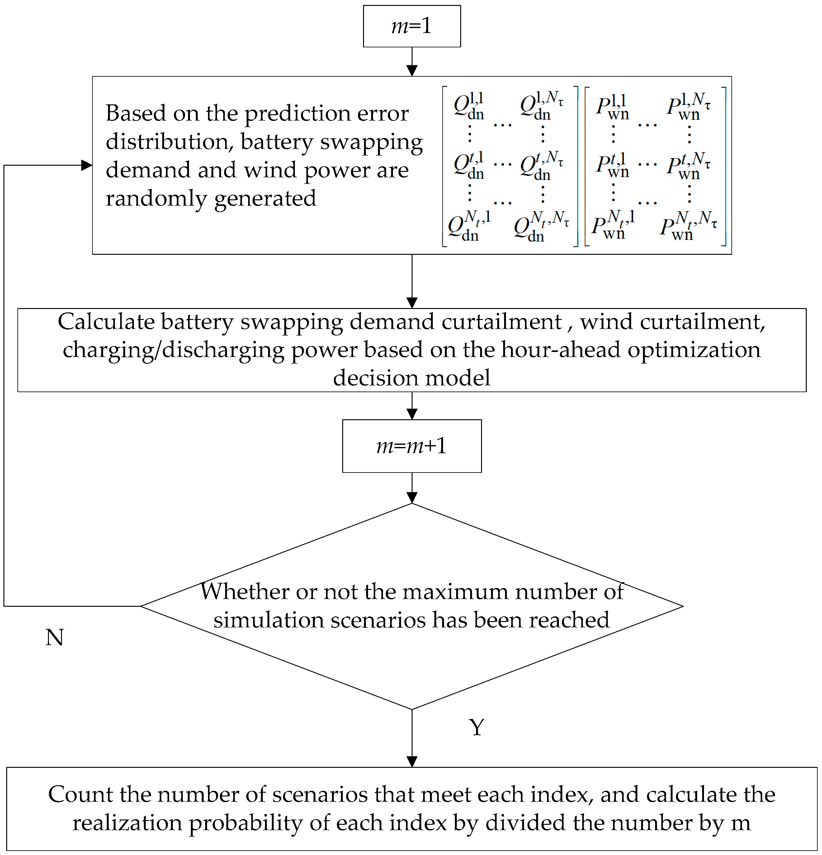
25]. MATLAB (R2012b, MathWorks, Natick, MA, USA, 2012) was adopted for solving the algorithm. The overall optimization of the model includes initialization, selection, crossover and mutation operation, which is the same as the traditional genetic algorithm. The special feature is the calculation of fitness function of GA. Since the fitness is realization probability of the indices, it should be solved by means of stochastic simulation. The flowchart of the stochastic simulation is shown in
Figure 1.
Under a stochastic simulation scenario, if wind power and battery swapping demand within each hour are replaced by only one set of simulation values, the accuracy level is not sufficient, which is detrimental to explore the reserve capability of the BSS. Therefore, during the stochastic simulation, further optimization adjustment procedure of the BSS within each hour should be taken into consideration to address the random fluctuations of wind power and battery swapping demand. In other words, the hour-ahead optimization decision process should be considered. Furthermore, each hour is divided into Nτ time intervals. According to the day-ahead prediction of wind power and battery swapping demand as well as the probability distribution of their prediction error, m groups of scenarios are generated randomly to simulate the fluctuations of wind power and battery swapping demand. In addition, the hour-ahead optimization decision model is employed to calculate the optimization solution. In line with the law of large numbers, when m is large enough, the probability satisfied by such an operating index can be approximately replaced by the proportion taken by the number of scenarios satisfying the operating index in the total quantity of simulation scenarios.
5. Hour-Ahead Optimization Decision Model
The hour-ahead optimization decision model is carried out every hour in a rolling manner based on the ultra-short term prediction of wind power and battery swapping demand. The corresponding objective function is:
The objective function consists of three parts. The first part stands for battery swapping demand curtailment; the second part stands for wind curtailment; and the third part stands for the output power of integrated system beyond the permissible range δ. Nτ is the number of time intervals for each hour during ultra-short term prediction; Δτ is the time interval; and ρ1, ρ2 and ρ3 are weighting factors. The decision variables include the battery swapping demand curtailment , wind curtailment power , charge power and the discharge power .
Considering that battery swapping requires some time, the energy stored in the batteries that need to be swapped within every hour no longer participates into the decision-making process. At the very beginning of the hour
t, the initial energy storage
, which can be involved with such a process, can be expressed as:
where
is the battery swapping demand at time interval τ within the hour
t.
The expression for stored energy
of BSS at time interval τ can be expressed as
The hour-ahead optimization decision model is subject to Equations (22)–(30):
Constraints on storage capacity in the BSS
Constraints on energy storage in the BSS at the end of an hour
Constraints on battery swapping demand curtailment
Constraints on wind curtailment power
Constraints on charging/discharging power
As binary variables,
and
are charge and discharge flags. Moreover, Equation (29) represents that the integrated system does not purchase power from the power grid.
Constraints on the maximum relative error between output power of the integrated system and generation schedule.
where
is the maximum permissible absolute value of relative error.
Through introducing an intermediate variable to replace the third part of objective function, the hour-ahead optimization decision model can be transformed into a mixed-integer linear programming model, which can be solved by state-of-art commercial solvers such as CPLEX (12.3, IBM, Armonk, NY, USA, 2010).
6. Simulation Analysis
In the study cases, multiple wind farms and a number of BSSs in the model are aggregated into one wind farm and one BSS. The equivalent wind farm data is selected from a wind farm in Shandong Province and its installed capacity is 99 MW. The parameters of the BSS for EVs are obtained from a practical station in this province and they are shown in
Table 1. Both
Qini and
Qend are set as 50% of the maximum storage capacity of the BSS.
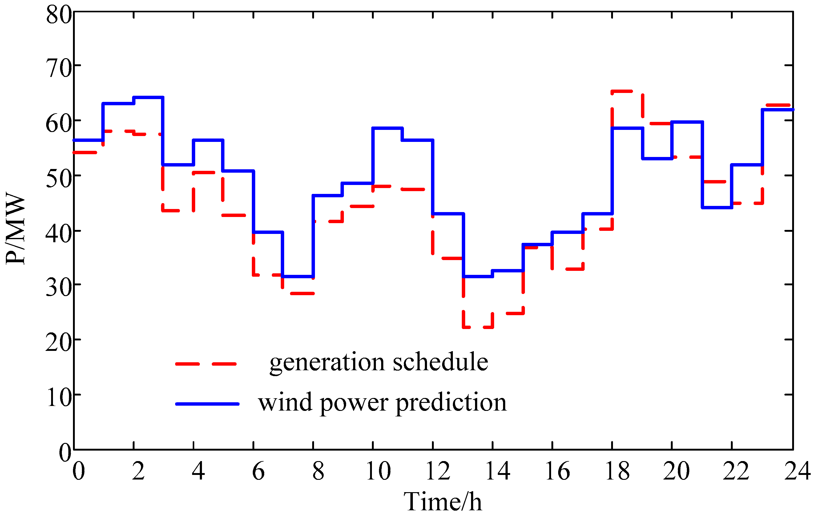
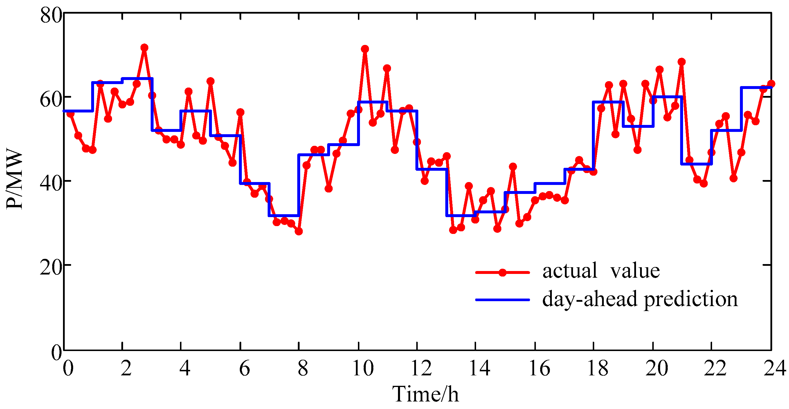
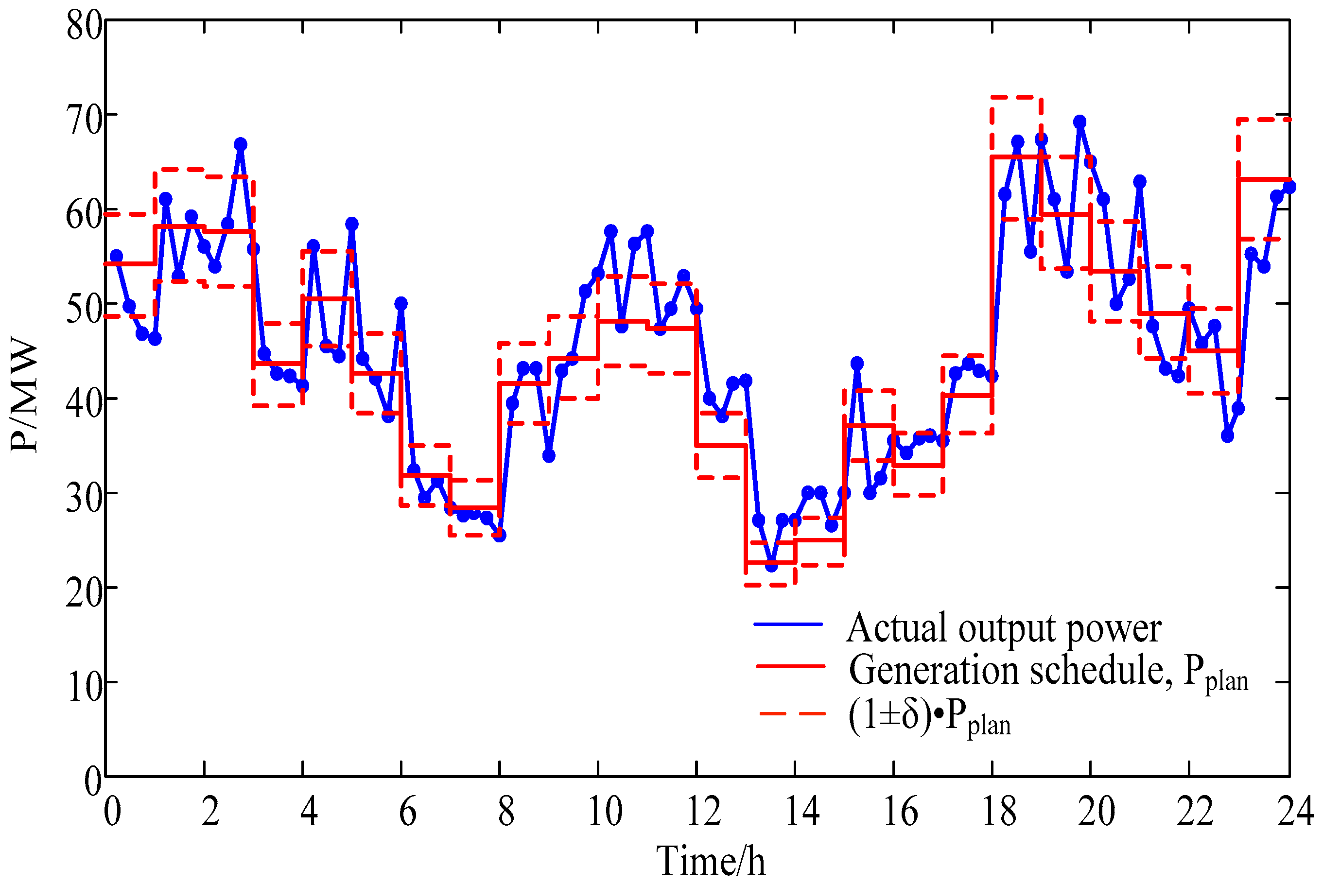
In
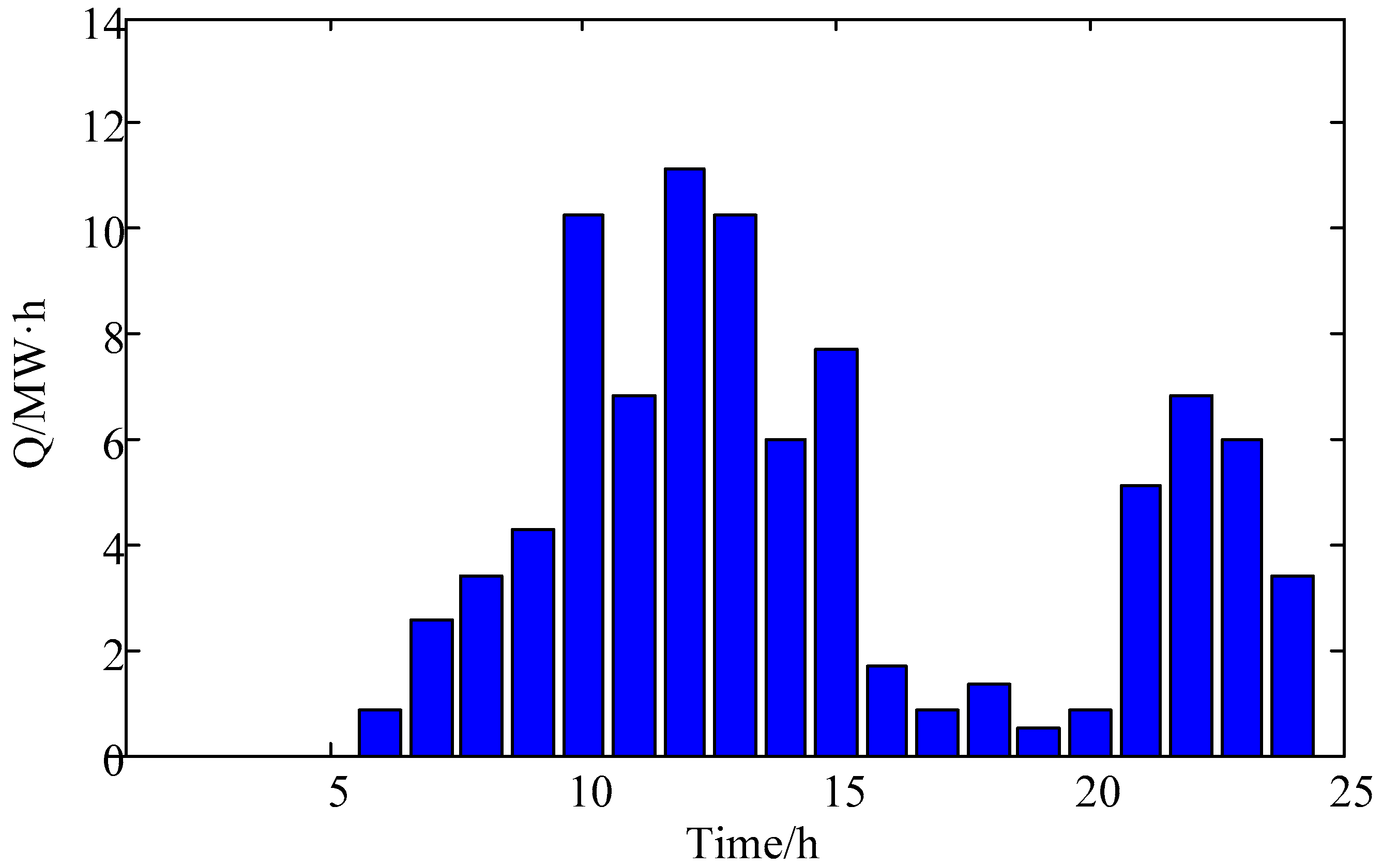
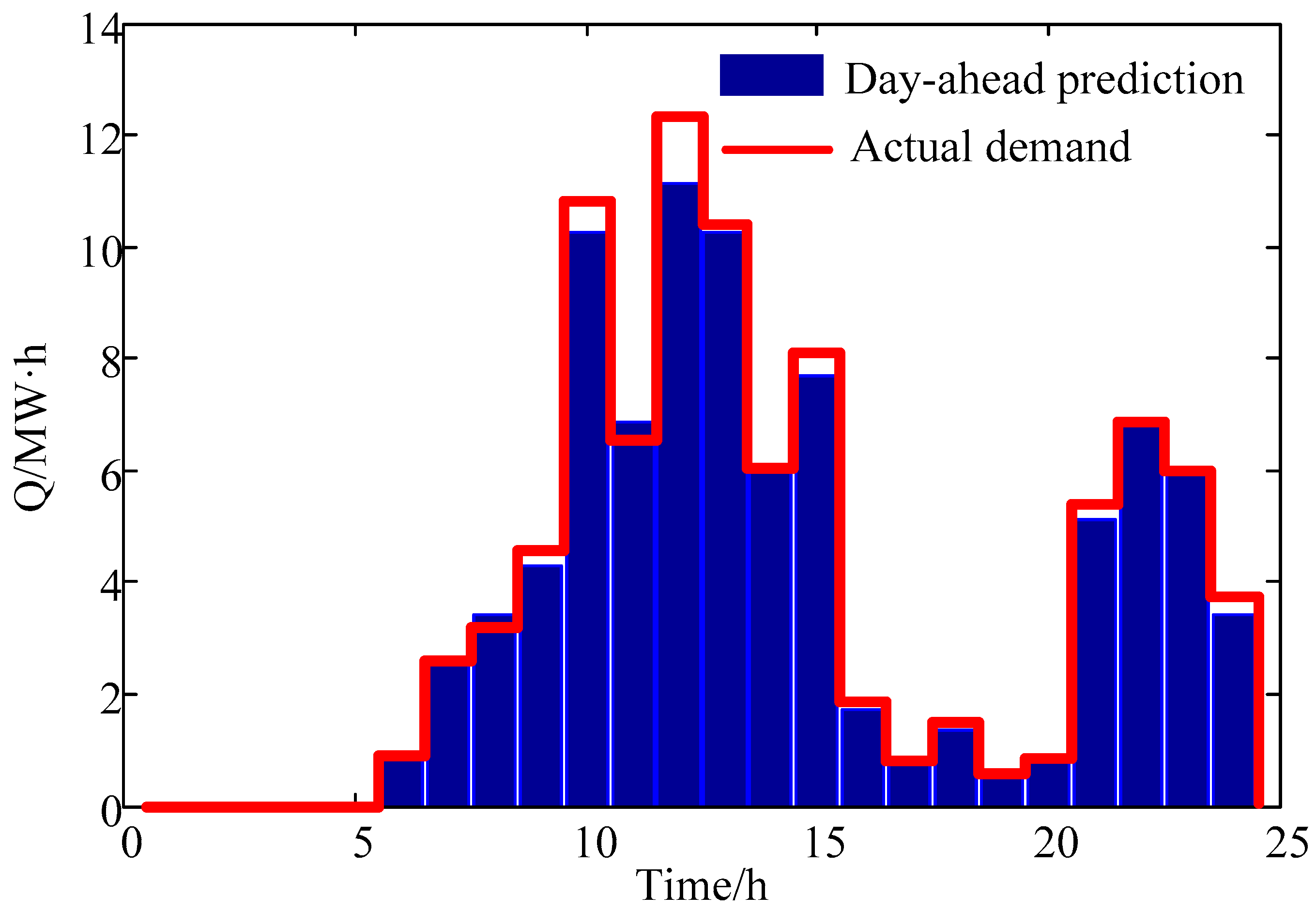
Figure 2, the day-ahead wind power prediction and the generation schedule of the integrated system are presented. The day-ahead prediction of battery swapping demand is shown in
Figure 3. Studied in [
21,
26], the random fluctuations of wind power and EV power demand obey normal distribution N(0, σ
2), where the probability in [3σ, −3σ] is 99.73%. Based on the historical data, we found that the relative prediction error of wind power and battery switch demand is no more than 30%. Therefore, we assume that the relative prediction error of day-ahead prediction for wind power and battery swapping demand all follow the normal distribution of N(0, 0.1
2). It should be noted that the distribution of the prediction error will not affect the use of the model proposed in this paper, what we need to do is just modify the stochastic simulation process in
Section 4 accordingly.
The decision-making cycle for day-ahead collaborative scheduling is 24 h of the next day and one hour is seen as one interval. For the hour-ahead optimization decision, the cycle is 1 h in the future and every 15 min is seen as an interval. Therefore, there are four intervals in hour-ahead model.
In general, wind farms and EVBSSs have their own operation objectives, thus the desired values of the indices could be set accordingly. The maximum permissible battery swapping demand curtailment Qds is 0.1 MW·h, 1‰ of cumulative daily battery swapping demand. The maximum wind curtailment Qws, which takes 1‰ of the cumulative daily generated energy of a wind farm, is 1.2 MW·h. δ and α are 10% and 20%, respectively. In addition, the priority order and target values for realization probabilities of three operating indices should be reasonably set according to the decision-maker’s preference to different indices and the level of risk tolerance as well. In this paper, the priority ranking of the operating indices from high to low is the index of battery swapping demand curtailment, wind curtailment and generation schedule tracking. Target values for their realization probabilities are 97%, 90% and 90% respectively.
According to the above conditions, the day-ahead collaborative scheduling was performed. The parameters of the genetic algorithm are set as follows: crossover rate is 0.4, mutation rate is 0.2, size of the population is 50 and the maximal iteration number is 300. The computed realization probabilities of the three indices are 97.0%, 89.1% and 89.0%. The energy storage in BSS is presented in
Figure 4.
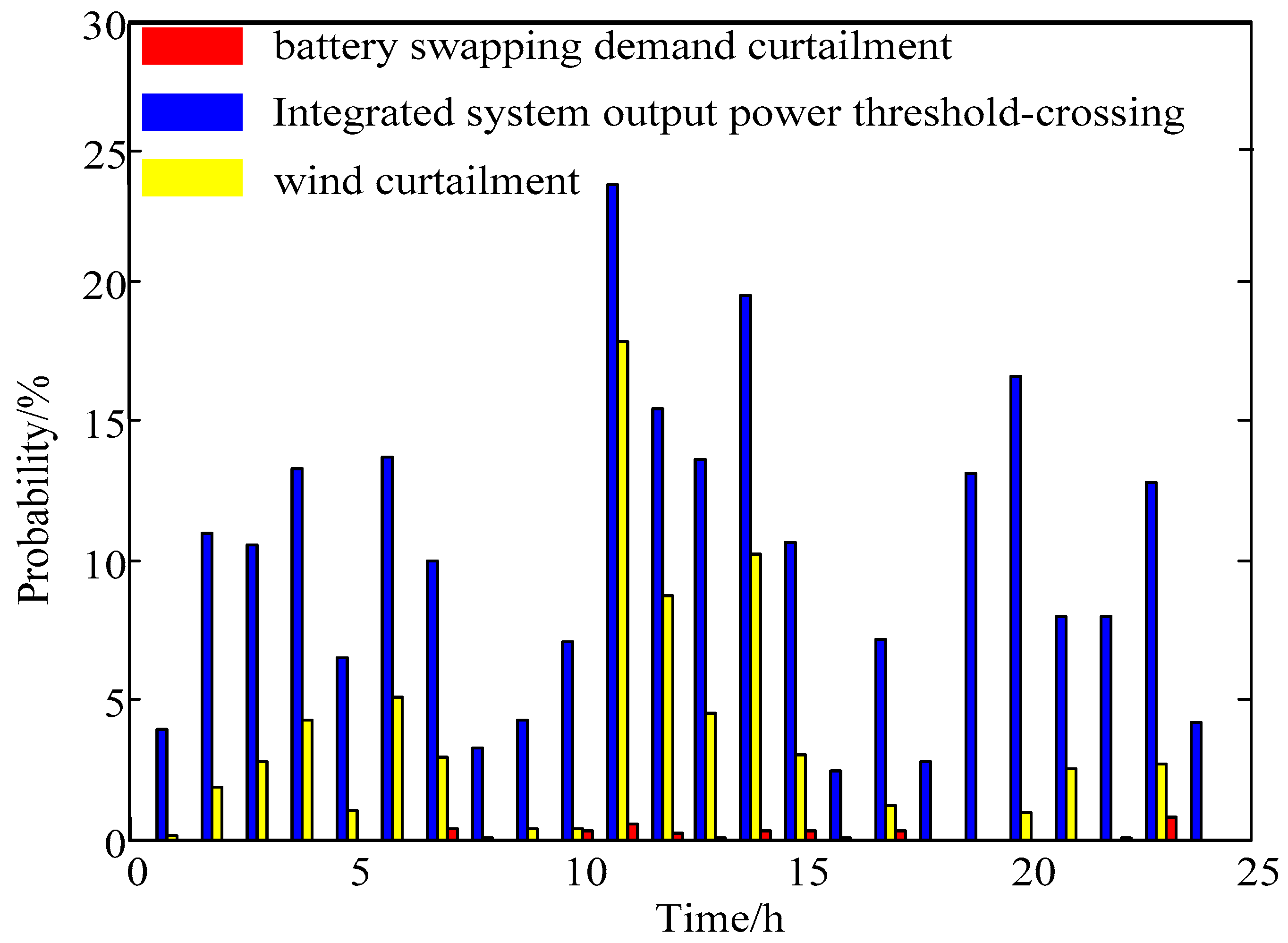
The probabilities for battery swapping demand curtailment, wind curtailment and integrated system output power threshold-crossing (that is, the absolute value of relative error between integrated system output power and generation schedule is greater than
) to take place at each time interval are given in
Figure 5.
From this figure, it can be seen that it is least likely for battery swapping demand curtailment to occur in each time interval and the relevant probabilities are no more than 1%. At time interval 11 and 14, the probability of wind curtailment exceeds 10%. Probabilities for integrated system output power threshold-crossing are rather high, which goes beyond 15% at interval 11, 12, 14 and 20. The results were closely related to the priority order of three operating indices. Since the index of battery swapping demand curtailment has a higher priority than the other two indices, the model would give priority to meet the battery swapping demand, and the probability of battery swapping demand curtailment is correspondingly the lowest. Similarly, power threshold-crossing is more likely to take place because it has the lowest priority.
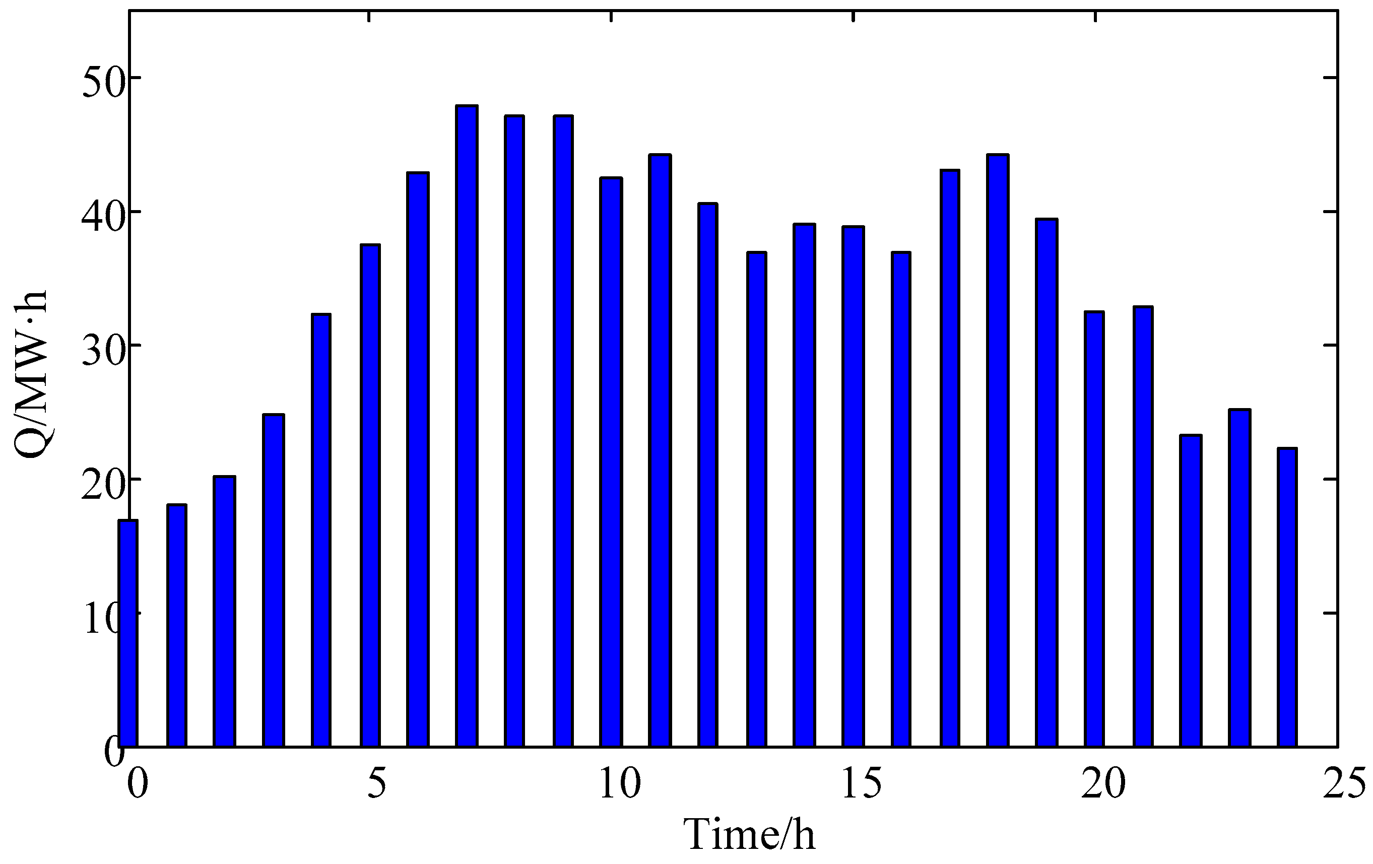
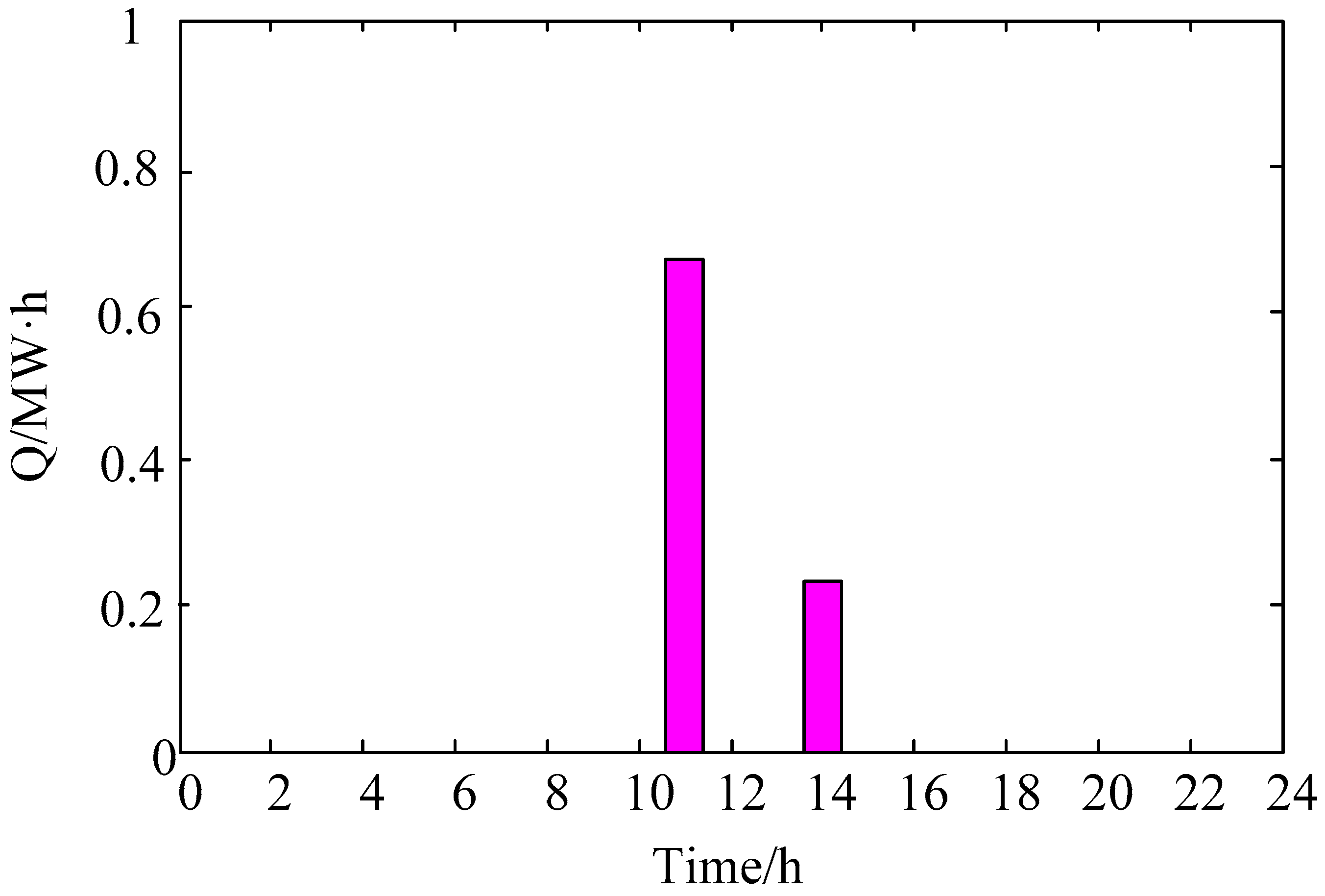
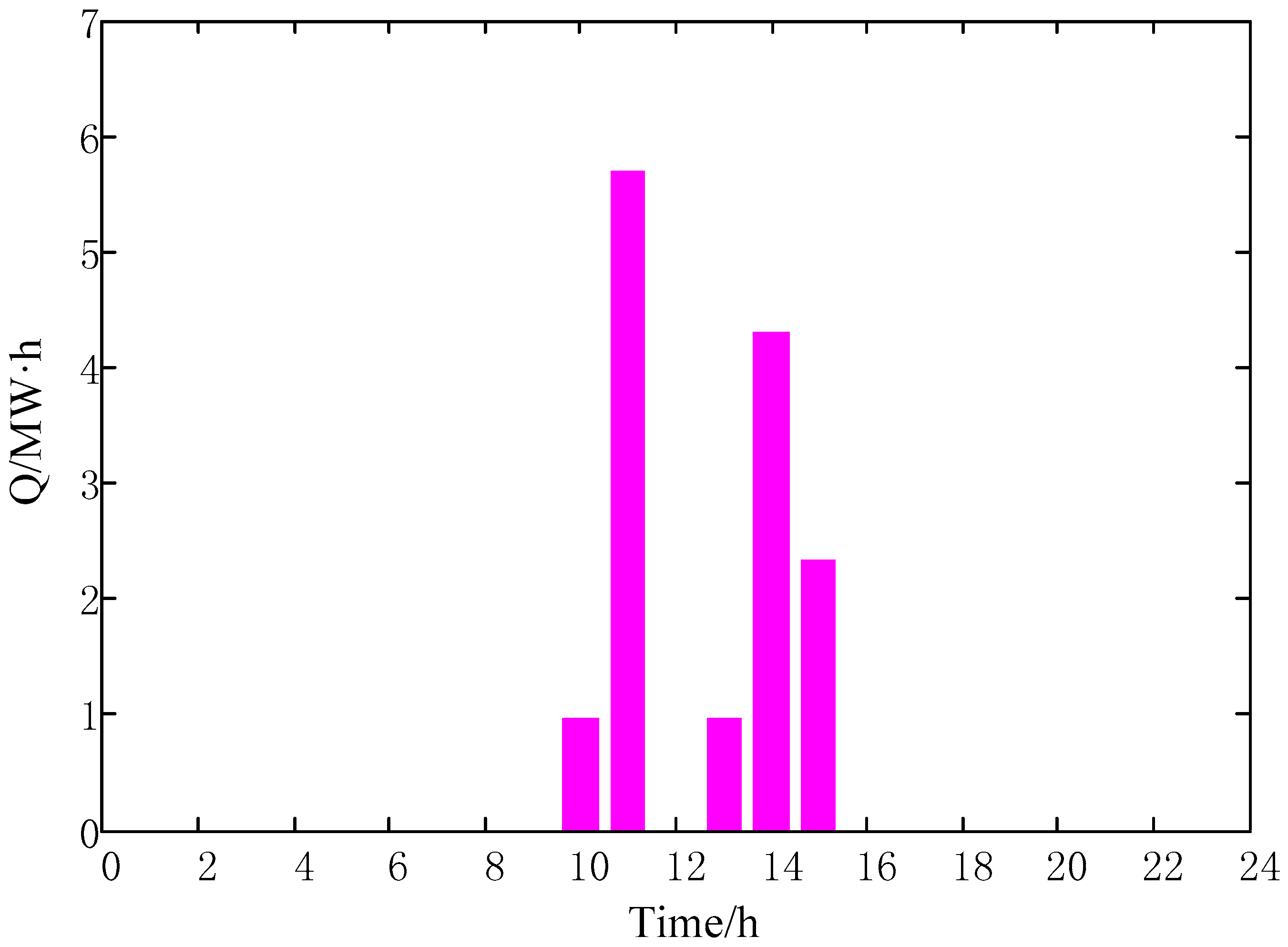
The hour-ahead optimization decision model can be adopted to verify the above results. Ultra-short term prediction of battery swapping demand and wind power are respectively replaced by the actual battery swapping demand (shown in
Figure 6) and the actual wind power (shown in
Figure 7). After calculation, the battery swapping demand curtailment is 0 MW·h. Besides, the wind curtailment is 0.86 MW·h that appears at interval 11 and 14 (shown in
Figure 8), which shows consistency with outcomes given in
Figure 5.
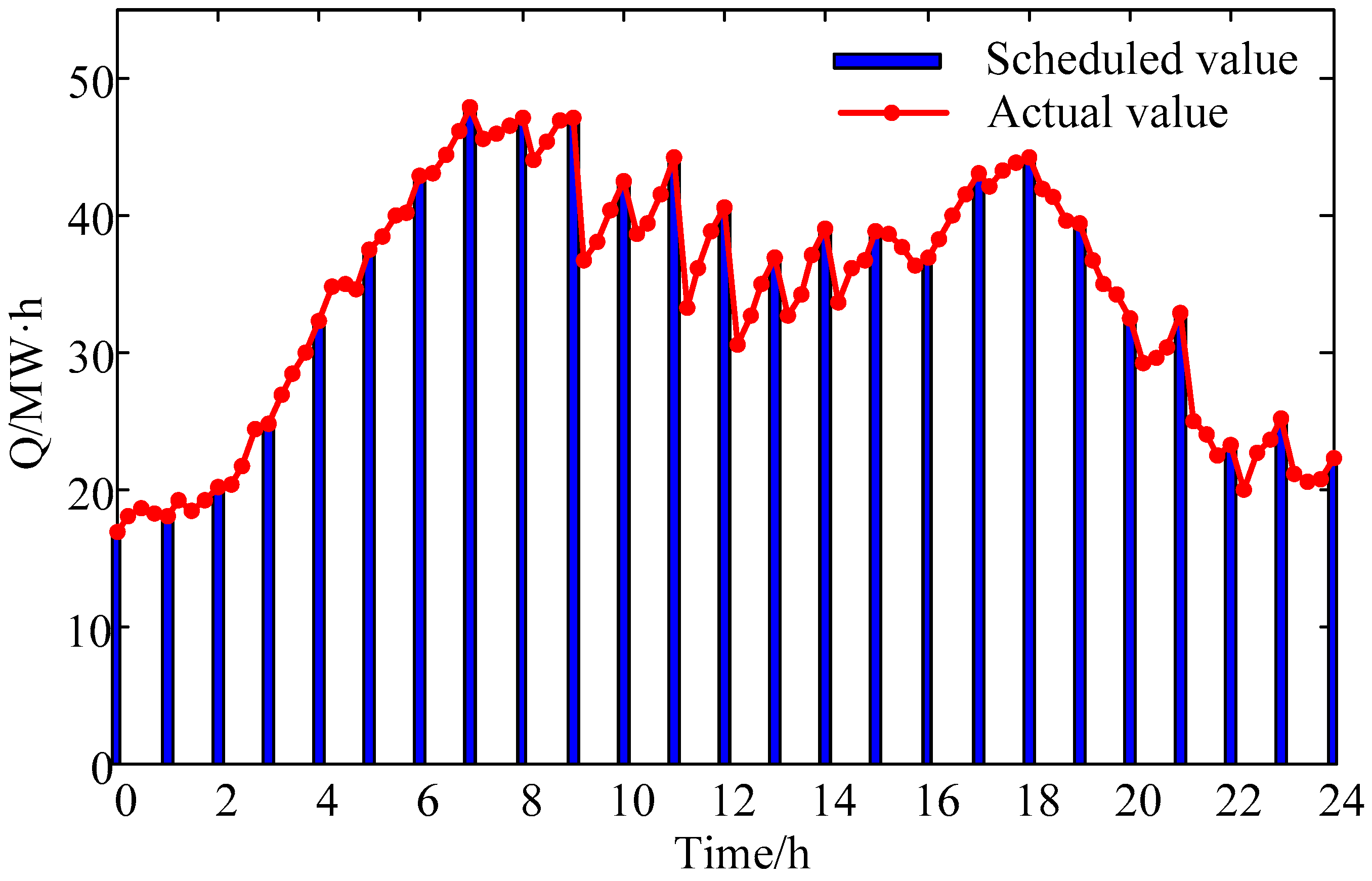
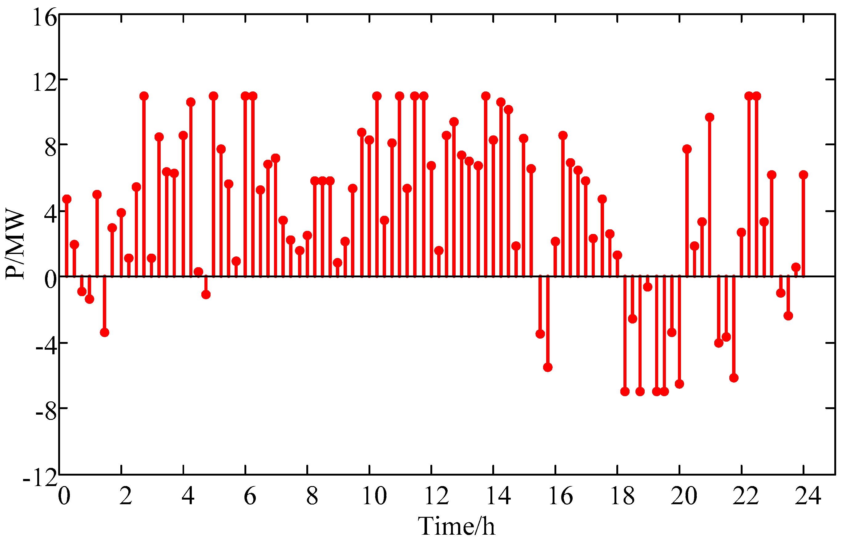
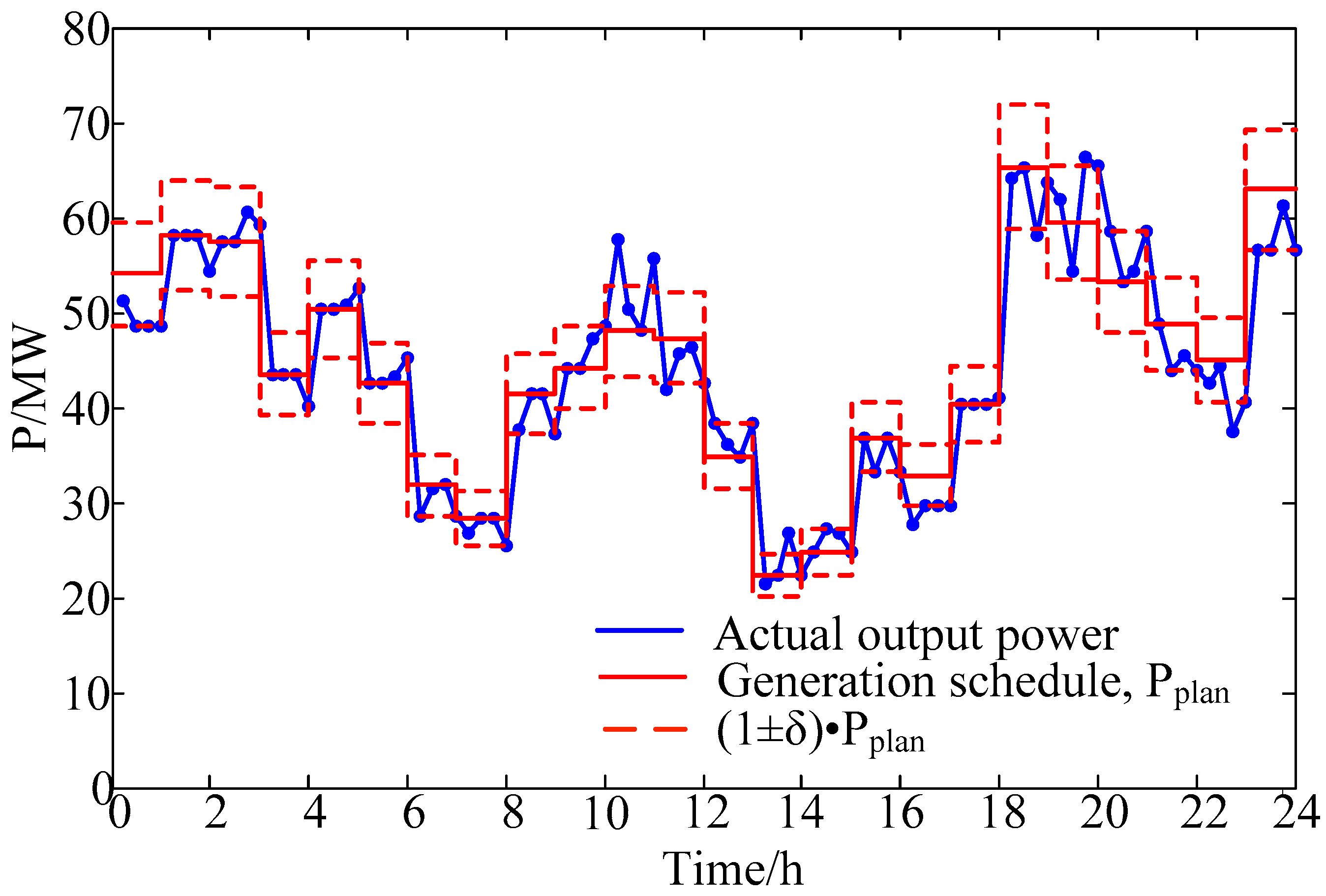
The actual output power of the integrated system is given in
Figure 9. As a whole, the integrated system preferably follows the corresponding generation schedule. However, at interval 11, 14, 17, 20 and 23, a poor tracking situation occurs and power threshold-crossing takes place. As the actual wind power is substantially different from the day-ahead prediction for such four intervals, the power threshold-crossing still occurs to the integrated system output despite that the charging/discharging regulations are performed within the permissible range for the BSS with limited regulation capacities. The time intervals when threshold-crossing takes place basically conform to those with higher probabilities for threshold-crossing occurrence given in
Figure 5.
Figure 10 presents variations in actual stored energy of the BSS. Clearly, the day-ahead collaborative scheduling model can optimize the BSS regulation capacity from a global perspective, and it determines the readjustment limits for the charging/discharging powers at various time intervals. As a result, the energy storage of the BSS could be prevented from reaching its upper/lower limits during the beginning several intervals, and avoiding the situation that the BBS losing its regulation capacities in the subsequent periods.
Figure 11 represents the charging/discharging power of the BSS. Within each hour, the hour-ahead optimization decision is able to regulate charging/discharging power of BSS to deal with fluctuations in wind power and battery swapping demand. If only the day-ahead collaborative scheduling is considered, the hourly charging/discharging power readjustment is not taken into account, which means that the number of time interval for the hour-ahead optimization decision is one, and the charging/discharging power of the BSS in each hour is a fixed value. Since the BSS has lost the ability to adjust further within each hour, the wind power fluctuation will result in a significant increase in the probabilities of wind curtailment and integrated system output power threshold-crossing, accordingly. In this situation, the battery swapping demand curtailment can be figured out as 0 MW·h. In addition, the wind curtailment is 14.4 MW·h which goes beyond the maximum permissible wind curtailment quantity
Qws (1.2 MW·h). Consequently, the second operating index is not satisfied. As for wind curtailment for all intervals, please refer to
Figure 12. The actual output power of the integrated system is given in
Figure 13.
Take the 15th hour as an example. The actual wind power is higher than the predicted value within the first 30 min and lower than the predicted value within the 30–45 min. Based on the model proposed in this paper, the BSS would increase the charging power within the first 30 min to absorb the surplus wind power, and would increase the discharge power within the 30–45 min to compensate for the wind power shortage. In this way, there was no wind curtailment and power threshold-crossing for the entire hour (shown in
Figure 8 and
Figure 9). However, for the model without considering charging/discharging power readjustment, the integrated system output power threshold-crossing took place due to lack of readjustment. In addition, it is necessary to curtail wind to prevent the output power from exceeding the maximum allowable deviation α.
Comparing
Figure 8 and
Figure 9 with
Figure 12 and
Figure 13, it is clearly found that the proposed model can deal with random fluctuations of wind power and battery swapping demand in a better manner compared with the one in which hour ahead model is not considered. The proposed model can also reduce the curtailment in battery swapping demand and wind power, and improve the tracking effect of the integrated system. Finally, the three operating indices can be satisfied more preferably.


 ,
, 


