1. Introduction
The main objectives for next generation communications, although they may be different for various organizations, are high data rate, low latency and low energy consumption [
1]. Data rate means not only average data rate but also cell edge data rate, which is the worst data rate, because of inter-cell interference. With the deployment of broadband data services, demands of mobile traffic are growing rapidly [
2], and thus the 4th generation wireless networks may reach their limits soon. This implies that the above-mentioned three objectives may not be achieved at the same time, and thus to resolve these challenges, research towards the 5th generation of mobile cellular networks is actively being conducted.
To improve user-perceived performance specifically focused on energy efficiency and cell edge users, many cell switch-off techniques have been proposed. The works in [
3,
4] proposed interference management schemes by switching off the nearest cells. The authors in [
5,
6] proposed inter-cell interference (ICI) management by exploiting adaptive fractional time reuse (FTR) instead of fractional frequency reuse (FFR). However, these works focused on improving edge user performance and neglected considering energy efficiency. A series of papers [
7,
8,
9,
10,
11,
12,
13] studied about energy-efficient cellular systems by switching off base stations and/or transmit antennas. The works such as [
14,
15] proposed energy harvesting wireless communication systems that exploit renewable energy such as solar power, wind power, etc. However, these works did not consider cell edge user performances. The work such as [
16] proposed increasing energy efficiency and cell edge user performances simultaneously by cell switch-off with coordinated multi-point (CoMP). The work such as [
17] proposed energy conservation and interference management in a multi-cell time division multiple access (TDMA) network. However, these works consider only the static system where the number of users are fixed, and thus cannot capture real systems where the number of users (or flows, equivalently) changes over time. The work such as [
18] studied energy and delay in the downlink of a proportional-fair cellular system with inter-cell interferences and fading. However, this work focused on the trade-off between energy and delay. To the best of our knowledge, increasing energy efficiency and cell edge user performances (or even improving the average performance of all users) simultaneously by cell switch-off, specifically in a dynamic system, has not been studied in the literature.
In this paper, we investigate a mechanism that improves three objectives at the same time, i.e., energy efficiency, cell edge user performances, and the average user performances by managing cell activation in a timely orthogonal fashion. We call it cell flashing because base stations are turned on and off periodically and rapidly so that, when one base station is turned on, the adjacent base stations that make interferences are always off; switching off adjacent cells significantly improves energy efficiency, and cell edge users obviously experience less inter-cell interference. Cell center users who were not experiencing much inter-cell interference, however, might be slightly penalized because the associated base station is not always on. Then, it becomes not clear, even though energy efficiency would be mostly improved with cell flashing, how overall system performance would be. In this regard, we are interested in under which circumstance cell flashing becomes beneficial for both energy efficiency as well as user-perceived performance (overall and/or in the cell edge). Note that, in general, switching off base stations to save energy leads to longer delay, i.e., there is a tradeoff between energy saving and user-perceived performance. Thus, a proper switching on–off mechanism and its theoretical analysis are essential.
One may think that cell flashing may not be practical, at least at this moment, because turning base stations on and off may take significant time, either base station (BS) goes to sleep mode or returns back to active mode, or uplink signals cannot be continuously received. When BS goes to deep-sleep mode, which consumes very low power, it takes a long time and uplink signals cannot be continuously received. However, when fast discontinuous transmission (DTX) is used [
19], the transition period between sleep mode and active mode is similar to the case of state on/off change in time division duplexing (TDD) system, and subframes for uplink signals can be continuously received at the expense of energy consumption [
20,
21]. According to [
22], it is possible to switch on/off states in the order of 17
s. This is a much shorter time than long term evolution advanced (LTE-A) scheduling period of 0.5 ms, and thus cell flashing can be viable. Of course, energy saving of DTX cannot be as much as that of deep-sleep mode.
To better understand energy saving and the user-perceived performance, we consider stochastic traffic loads where new file transfers, or equivalently flows, are initiated at random and leave the system after being served. This is usually referred to as flow-level dynamics [
23,
24,
25]. Unlike the previous works of FTR [
5,
6] where energy efficiency was ignored, and static population (or infinitely backlogged users) was assumed, our work is unique in the sense that it captures the impact of dynamic user population on energy efficiency and the long term average performance, which is closer to user-perceived performance, e.g., file download time (or called delay hereafter). Note that user experience is based on the time-averaged performance rather than instantaneous capacity. Analyzing such systems is, however, more challenging because of the dynamic nature of the system, and its analysis is hardly tractable in general [
24].
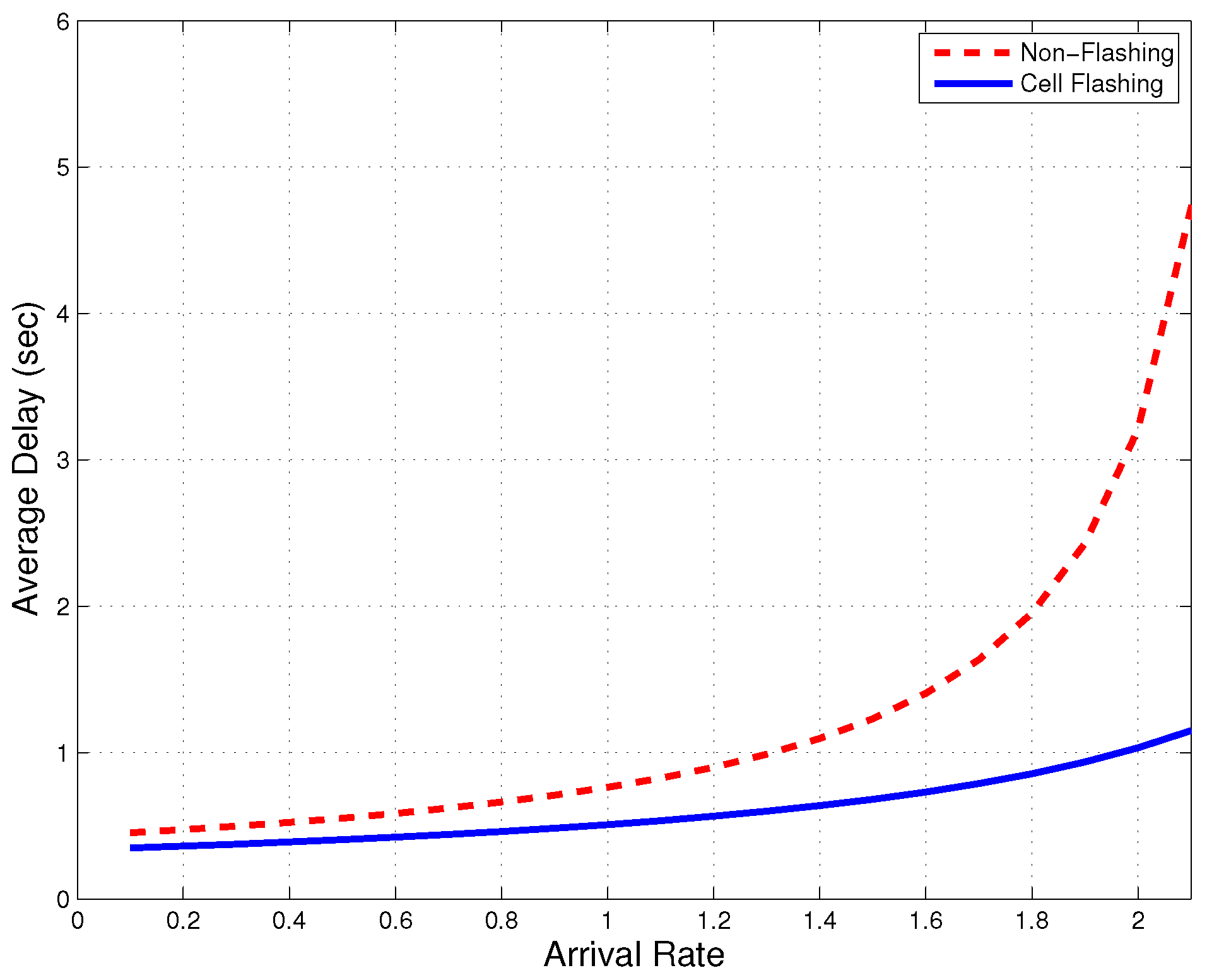
When cell flashing is employed in a dynamic system, we consider the user-perceived performance, i.e., the average delay measured by file download time and the energy consumption of base stations and formulate an optimization problem. Based on flow-level dynamics, we prove that cell flashing can improve both total energy saving and the average delay in the interference-limited regime, which is typically the case of small cells. This can be achieved because large average delay is mainly incurred by cell edge users’ poor performances, and thus improved cell edge user performances make the average delay lower. Thus, cell flashing has three advantages: higher energy efficiency, improved cell edge user performances, and lower average delay in small cells. These benefits are promising because cell densification is essential to achieve higher network-level capacity [
2] and lower energy consumption [
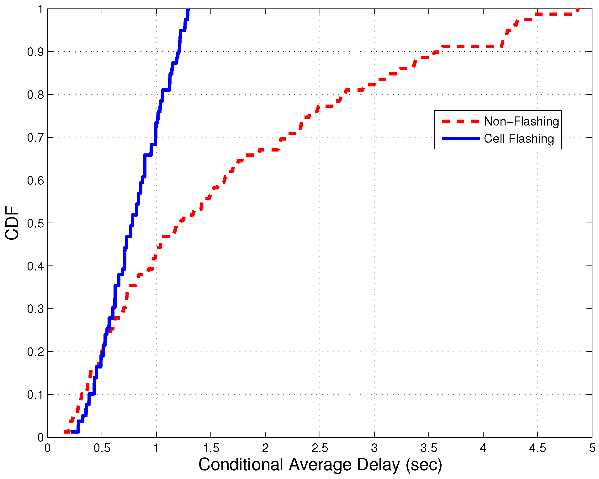
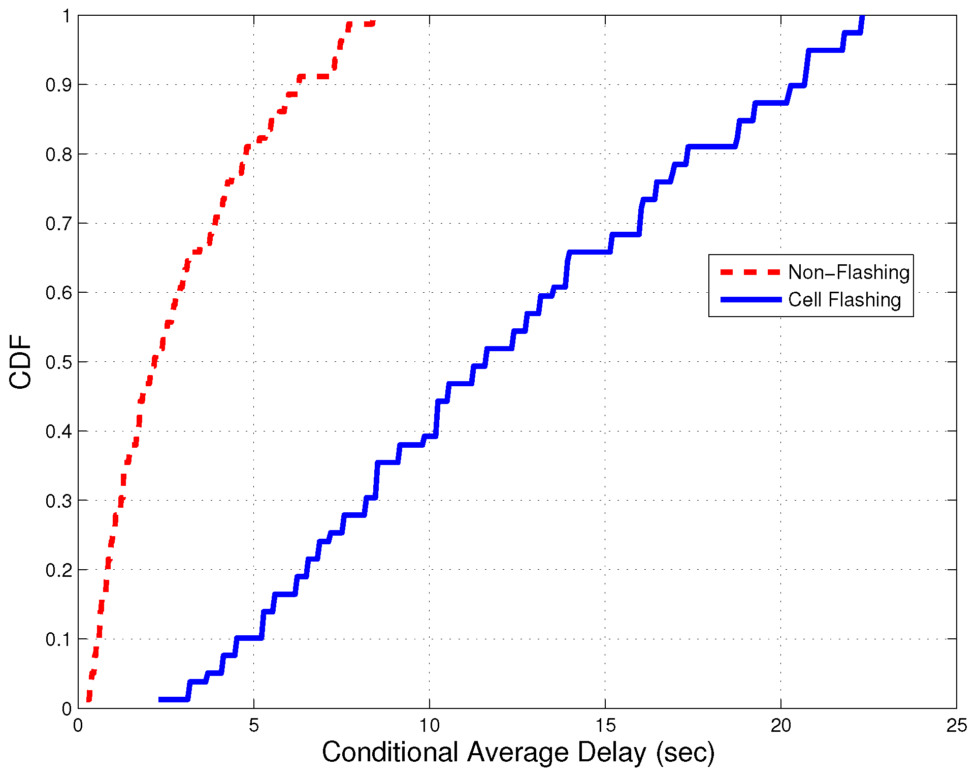
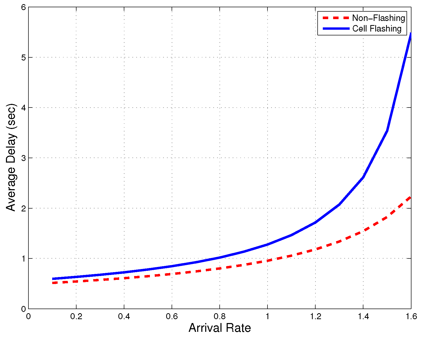
26]. However, as the cell radius increases, there is a tradeoff between energy saving and reducing delay. Our extensive simulations show that when noise power is negligibly small compared to transmit power, energy consumption of the base stations can be reduced by 25%, and at the same time, the overall average delay is reduced by up to 75% compared to the case of non-flashing. Furthermore, the performance improvement for cell edge users is also noticeable, e.g., the conditional average delay at cell edge is reduced by 80%.
We would like to emphasize that previous papers mainly focused on deep-sleep mode on a long-term scale, but our work analyzes the impact of turning BSs on and off rapidly while receiving uplink signals continuously. Thus, the time scales of energy saving are different, and cell flashing can be implemented independently of deep-sleep mode; even if the BS decides to remain on because traffic volume is moderate, the BS still can be turned on/off rapidly for extra energy saving. In addition, cell flashing can reduce both energy and delay simultaneously in small cells (see Proposition 1).
The rest of paper is organized as follows. In
Section 2, we describe the hexagonal cellular model used in our study. In
Section 3, we analyze the optimal delay and energy efficiency when cell flashing is used. In
Section 4, numerical results are given followed by conclusion in
Section 5.
2. System Model
We assume a basic small cell wireless network where each base station is equipped with an omnidirectional antenna. For analytical tractability, we consider small cell hexagonal networks, but our model can be further extended to randomly deployed small cells using stochastic geometry, which is beyond the scope of this paper. We consider a region
that is served by a set of base stations
. Let
denote a location and
be a BS index. Note that we use the BS index
i for cell index because BS and cell refer to the same object with slightly different purposes, which can be understood in the context. Let
be a
cluster, which consists of a set of adjacent cells that may orthogonally use a time-domain resource. Even though the number of the BSs in a cluster can be two or more,
three is meaningful in a practical system because too many BSs in a cluster sacrifice the benefit of frequency reuse. Thus, we consider three BSs in a cluster hereafter. We assume that file transfer or web page download requests, i.e., flow arrivals follow a Poisson point process with arrival rate per unit area
and file sizes that are independently distributed with mean 1/
at location
, so the traffic load density is defined by
; we assume
for
. This captures spatial traffic variability. For example, a hot spot can be characterized by a high arrival rate and/or possibly large file sizes [
23,
24,
25].
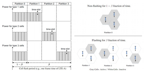
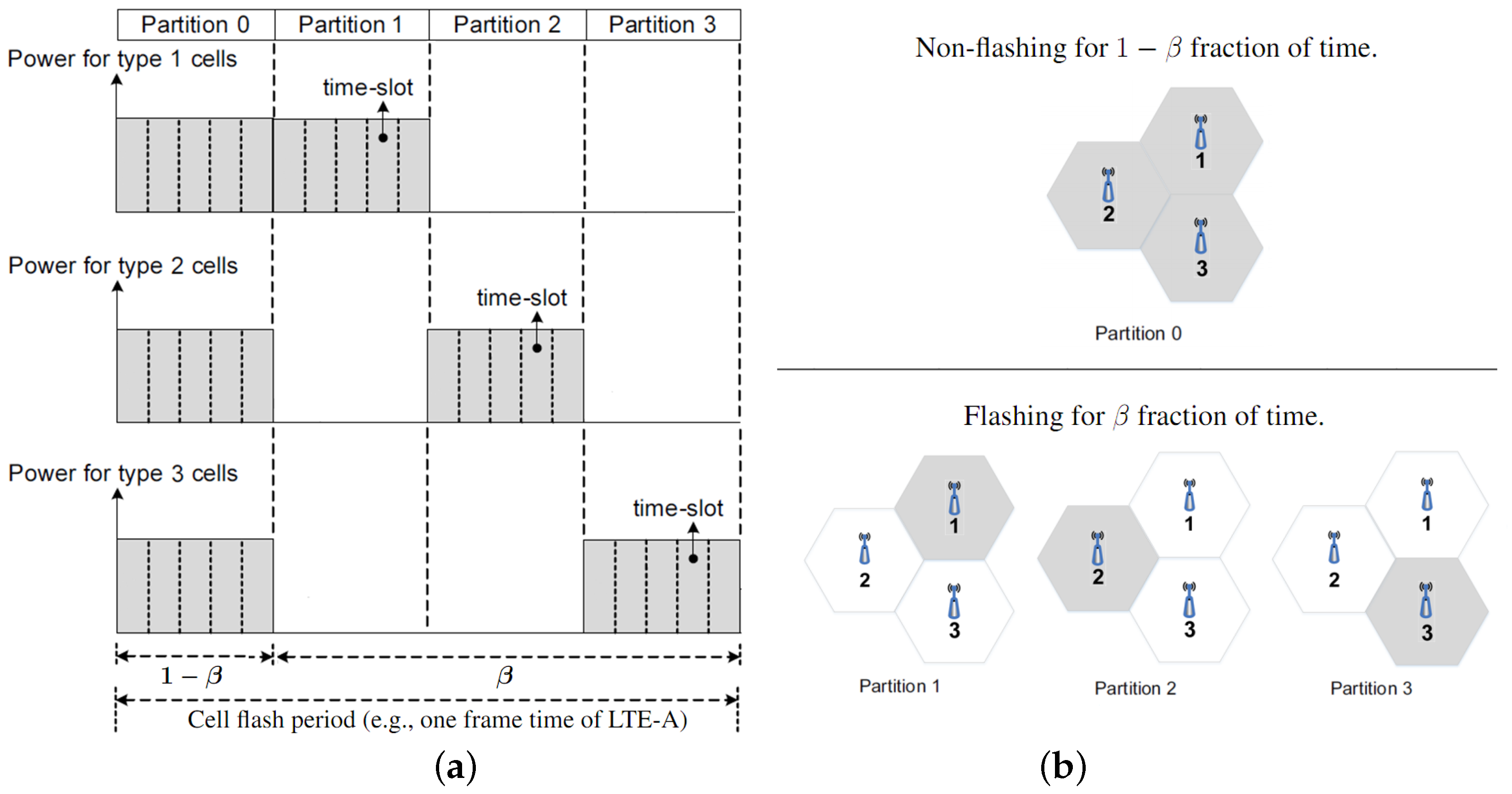
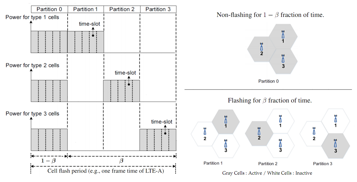
Figure 1 depicts the hexagonal cellular networks operated by cell flashing.
Figure 1a shows the case when time-domain resources are divided into four partitions. In partition 0, all three BSs transmit while in partition
i. Only BS
i transmits and other BSs remain silent.
Figure 1b shows the coverage based on signal-to-interference-plus-noise ratio (SINR) in each partition. For example, during partition 0, each cell serves its own coverage, while during partition
i, only BS
i is activated and serves its own coverage. Let
denote a fraction of time that cells flash, i.e., the fraction of time for partitions 1, 2, and 3. Thus, with a ratio of
, all BSs are on (partition 0), and with a ratio of
, only one BS
is on as shown in
Figure 1b. Thus, the inter-cell interference can be decreased just like frequency reuse 3, and capacity seen by cell edge users can be improved.
One may want to consider load balancing where radio resource, either time or frequency, is allocated depending on traffic variation in space. For example, our previous work of [
25] proposed adaptively changing the spectrum bandwidth of each BS in accordance with the loads of BSs. In this work, however, we do not consider load balancing because when partition time is not orthogonalized among adjacent clusters, inter-cluster interferences from adjacent clusters may become severe. This makes complicated dynamic inter-cell interference unavoidable, and the analysis of flow-level dynamics is not applicable [
24,
25,
27]. In this regard, we consider the case where all cells have the equal partition length. The study on cell flashing with load balancing remains for further study.
This paper focuses on scenarios where users see (a roughly) static interference from neighboring cells, which was also assumed in [
23,
24,
25]. Static interference assumption makes sense when interfering cells independently operate with the interfered cell and also interferences are not severe by using, for example, FFR or enhanced inter-cell interference coordination (eICIC). Then, the summation of interference can be considered as static Gaussian-like noise [
23,
24,
25].
We use Shannon capacity to model the transmission rate to a user at location
x, i.e.,
where
W denotes the channel bandwidth, and
is the receive signal-to-interference-plus-noise ratio at location
x for the signal from BS
i. For analytical tractability, we assume that
does not change over time, i.e., we do not consider fast fading or dynamic inter-cell interferences. Instead,
can be considered as a time-averaged transmission rate. This assumption is reasonable when the time scale for measuring channel gain
is assumed to be much larger than the time scale of fast fading [
23,
24].
is then given by:
where
denotes the transmission power spectral density (W/Hz) of BS
i,
denotes the total channel gain from the BS
i to the user equipment (UE) at location
x, including path loss, shadowing, and other factors, if any. In addition,
denotes noise power spectral density (W/Hz) and
denotes the average interference power spectral density seen by the UE at location
x.
Assumption 1 (fast flashing)
. We assume that the cell flashing is much faster than flow arrival process, which is reasonable because one frame time in LTE-A is 10 ms, which is much shorter than average file download time that spans seconds to minutes. In addition, we consider that cell flashing period is one frame time of LTE-A or less.
Then, transition time between active and sleep mode becomes negligible because transition time in DTX is 17
s according to [
22]. We can operate cells with non-flashing or flashing mode. If
is 0, all base stations are always on, i.e., non-flashing, and this is same to the case of full time reuse. If
is 1, cellular networks always operate with cell flashing, and each base station is on one third of time in a timely orthogonal fashion. Let
denote the instantaneous capacity at location
x when cells are non-flashing and
denote the instantaneous capacity when one of three cells are on. Thus, the time-averaged capacity
at location
x with flashing ratio
is given by:
It should be noted that
is location-dependent but not necessarily determined by the distance from the BS
i. For example,
can be very small in a shadowed area where
is very small. Hence,
can capture shadowing as well [
25]. According to Assumption 1, we can use the time-averaged capacity Equation (
3) to define the system-load density as below:
which denotes the fraction of time required to deliver traffic load
from BS
i to location
x. We assume that
is finite, i.e., at least one BS has physical capacity to location
that is not arbitrarily close to zero [
25]. Then, the load of BS
i (or utilization) is given by:
where
is the coverage of BS
i. Note that the meaning of
is the busy fractional time of BS
i. We do not consider the unstable system, so
will be smaller than 1 [
25].
The system can be modeled by an
multi-class processor sharing system, which reflects the fact that users see different service rates and file sizes based on their locations [
24]. We also consider infinitely many classes because we address this problem in a continuous space
. The average number of flows at BS
i is then simply given by
and total number of flows in all base stations is
[
28]. From Little’s formula, minimizing the average number of flows is equivalent to minimizing the average delay experienced by a typical flow. Minimizing
is equivalent to minimizing
because
, which serves as one part of our objective functions in Equations (
6) and (
8).
Our notations are summarized in
Table 1.
3. Optimal Flashing Ratio
Our problem is to find an optimal flashing ratio
so as to minimize the system cost function given below. Let the average delay be
, which is given by:
Let the average total power consumption be
. From [
23], we know that power consumed by operating BS
i is
, where
denotes the transmit power, and
denotes static power when BS operates. Power consumed by sleeping BS is
. Note that BS is on with the fraction of
, so
is given by:
We then formulate our problem as optimization as follows.
Problem:
where
is the parameter that balances the tradeoff between delay and energy consumption. We analyze
and
first to investigate under which circumstance the optimal
can be found. Since all base stations are symmetric, we consider BS
i in analysis hereafter.
Lemma 1. is a convex function of .
Proof. To check the convexity, we obtain the second order derivatives of
, which is given by:
We then obtain the second order derivatives of
, which is given by:
Then, since and for , , we have . Thus, it is obvious that , which completes the proof. ☐
Lemma 2. is a monotone decreasing function of , and we have: Proof. The derivative function of
is:
From Equation (
5), we can obtain the coefficient of
in Equation (
13):
Note that
and
because of the reduced interference power. Then, it is obvious that the coefficient of
in Equation (
13) is negative and because operating power is larger than sleep power, the derivative function of
is negative, which completes the proof. ☐
From Lemmas 1 and 2 we now know that is a convex function of and is a monotone decreasing function of . Hereafter, we are interested in under which circumstance the optimal solution can be obtained. As one special case, we are interested in when the optimal is 1, i.e., cell flashing all the time is optimal. The following proposition is about cell flashing in interference-limited regime.
Proposition 1 (Cell flashing in interference-limited regime)
. Suppose that the traffic load density is uniform, i.e.,
for
. Then, in the interference limited regime,
is a monotone decreasing function, i.e.,
Proof. Since all base stations are symmetric, we focus on BS
i in the analysis hereafter. Let the path loss factor be
,
be the location of BS
i and
be the set of turned-on base stations when cells flash. Then, for any
,
and
are given by:
Note that in the interference limited regime, transmit power of the transmitter and the interferers are canceled out. Then, we obtain
as follows:
From Equation (
18), we can obtain the derivative function of
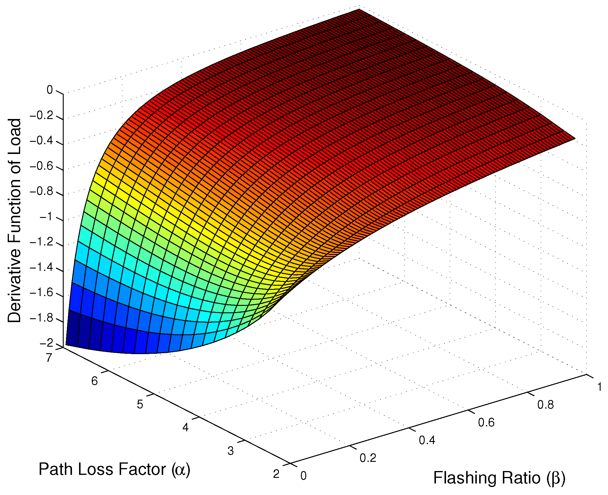
as follows:
Figure 2 shows
is negative for all
where the path loss factor is
[
29]. We are only interested in whether
is negative or not, so we set
and
. Thus,
is also negative for all
and we can know that
is a monotone decreasing function in
. It should be noted that we numerically check that
even when
is unrealistically high, e.g., 20. Since we verify all practically meaningful
, we do not attempt to prove that
holds for all
. ☐
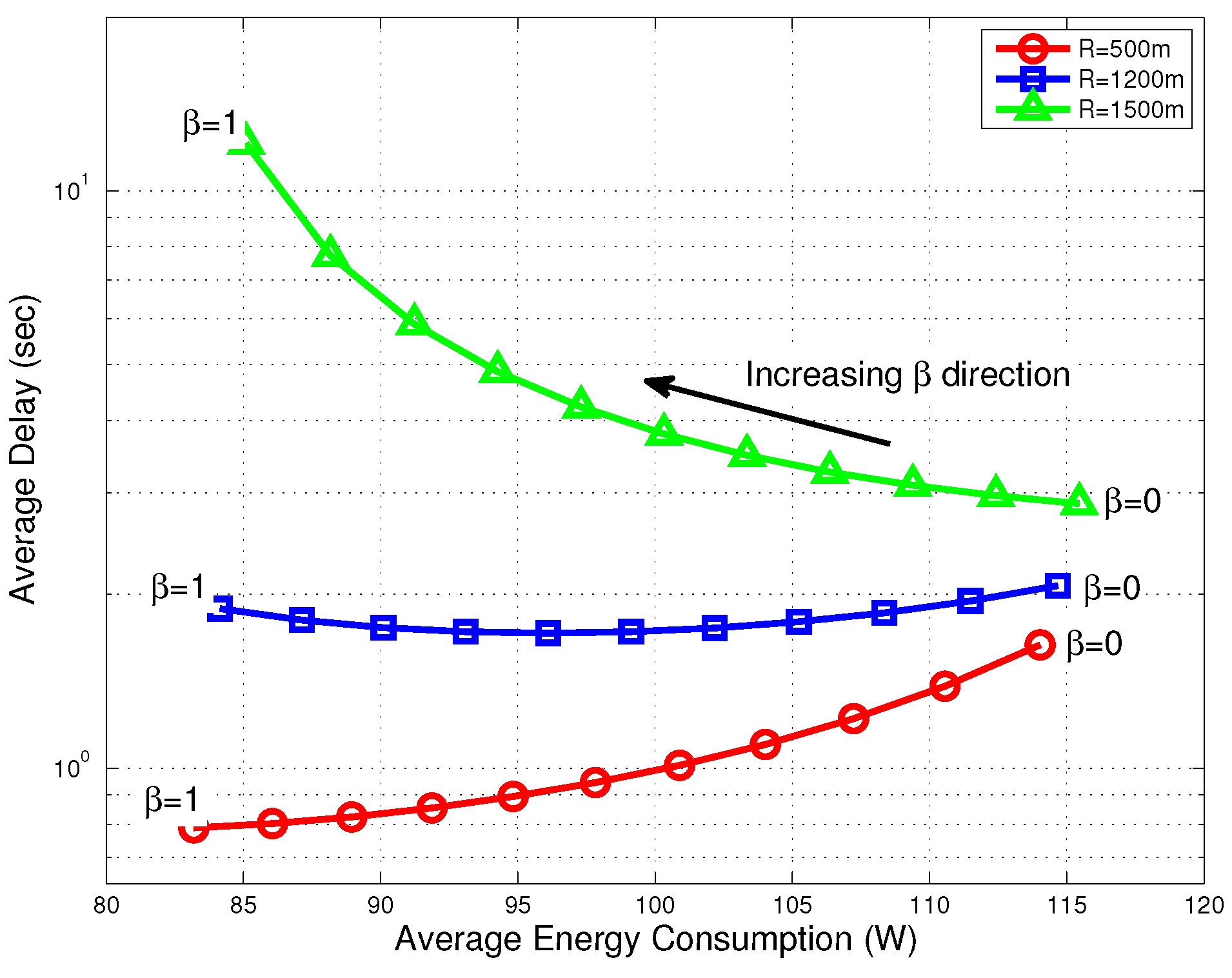
Remark 3.1. Note that by cell flashing, we can minimize average delay and average energy consumption simultaneously in the interference limited regime. Interference limited regime is usually the case with small cells. Furthermore, in 5G communication systems, cell coverage will be smaller than now for high data rates and low energy consumption, and thus cell flashing achieves both of them as well as improves the edge user performances.
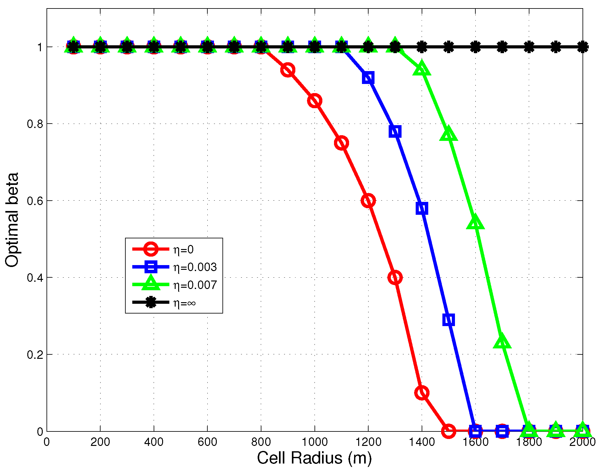
Remark 3.2. When the effect of the noise is high enough, the problem becomes non-trivial because can be an increasing function. In Section 4, we consider the impact of noise throughout all simulations. Remark 3.3. In general, is not a convex function. However, if is negligible in Equation (7), which means is much larger than , can be considered as a decreasing linear function [30]. Thus, becomes a convex function, and we can easily find the optimal . It is a reasonable assumption because is much larger than in small cells (see Table 2), and lies between 0 and 1. However, when is not negligible, the optimal can be found by exhaustive search; this may not be technically challenging because there is only one optimization variable. 


