Wave Tank Testing and Model Validation of an Autonomous Wave Energy Converter

Abstract

A key component in bringing ocean wave energy converters from concept to commercialization is the building and testing of scaled prototypes to provide model validation. A one quarter scale prototype of an autonomous two body heaving point absorber was modeled, built, and tested for this work. Wave tank testing results are compared with two hydrodynamic and system models—implemented in both ANSYS AQWA and MATLAB/Simulink—and show model validation over certain regions of operation. This work will serve as a guide for future developers of wave energy converter devices, providing insight in taking their design from concept to prototype stage.

1. Introduction

In order to fully realize a robust, efficient, and cost-effective ocean wave energy converter, considerable modeling and testing of devices will be required. Due to the size and complexity of the full scale devices, the most cost effective way to make advances is through the use of numerical modeling and scaled prototype testing. This paper takes previous numerical modeling work and attempts to validate these models with a scaled prototype tested in a large wave flume.

Wave tank testing of wave energy converters is a complicated endeavor with many challenges. There is much to be learned from previous attempts at characterizing devices and validating models. The European Marine Energy Centre (EMEC) provides a tank testing standard in [1] and the University of Edinburgh has provided tank testing guidance in [2] and EquiMar has provided high level guidance in [3]. The book edited by Joao Cruz [4], has a chapter dedicated to numerical and experimental modeling of Wave Energy Converters (WECs) which helped to inform the process of setting up the experiment, and identify best practices.

The main thrust of this research is to outline the process of taking an idea of a WEC and bringing it through the prototype stage of development. This includes a significant amount of numerical modeling as well as physical modeling. The outcomes of this paper show the results of tank testing, namely the Response Amplitude Operators (RAOs) and power performance results compared with two different time-domain model approaches. This model validation helps to identify the regions of operation that can be reasonably modeled, allows for the adjustment of the model to more accurately match the real world, and provides confidence to change the model for future design iterations.

There is considerable interest in the development of ocean wave energy converters for remote sensing applications [5]. In fact, there has been interest in this for some time. Yoshio Masuda was a pioneer in the field, creating an oscillating water column navigation buoy, commercialized in 1965 [6]. Currently, atmospheric sensing equipment on board remote buoys is typically powered by a combination of solar, wind, and battery systems. Point absorber wave energy conversion technology would add to the sensing system power options. To this end, a heaving two-body point absorber was chosen as a possible solution, called an Autonomous Wave Energy Converter (AWEC). A target power level for full scale development was set at a nominal 200 W.

2. Device Geometry, Scaling, Power Take Off, and Mooring

Many designs and geometry types exist for ocean wave energy extraction [6]. A heaving point absorber was chosen as the geometry to be modeled, built, and tested for this study. A point absorber is defined as a device whose horizontal extent is much smaller than one wavelength of an incoming wave. Energy conversion of point absorbers is limited by their heave only motion, however, benefits of this type of device include a relatively simple geometry, many previous studies and built devices based on this principle, and the robust nature of such a device.

2.1. Geometry

Full scale geometry design of the AWEC was outlined in [7], where coastal United States locations were chosen to help inform the design. A target of 200 W continuous power was chosen to meet the general electrical load of autonomous buoys. A focus on a simple shape was pursued for reasons of cost and ease of manufacture as well as ease of modeling.

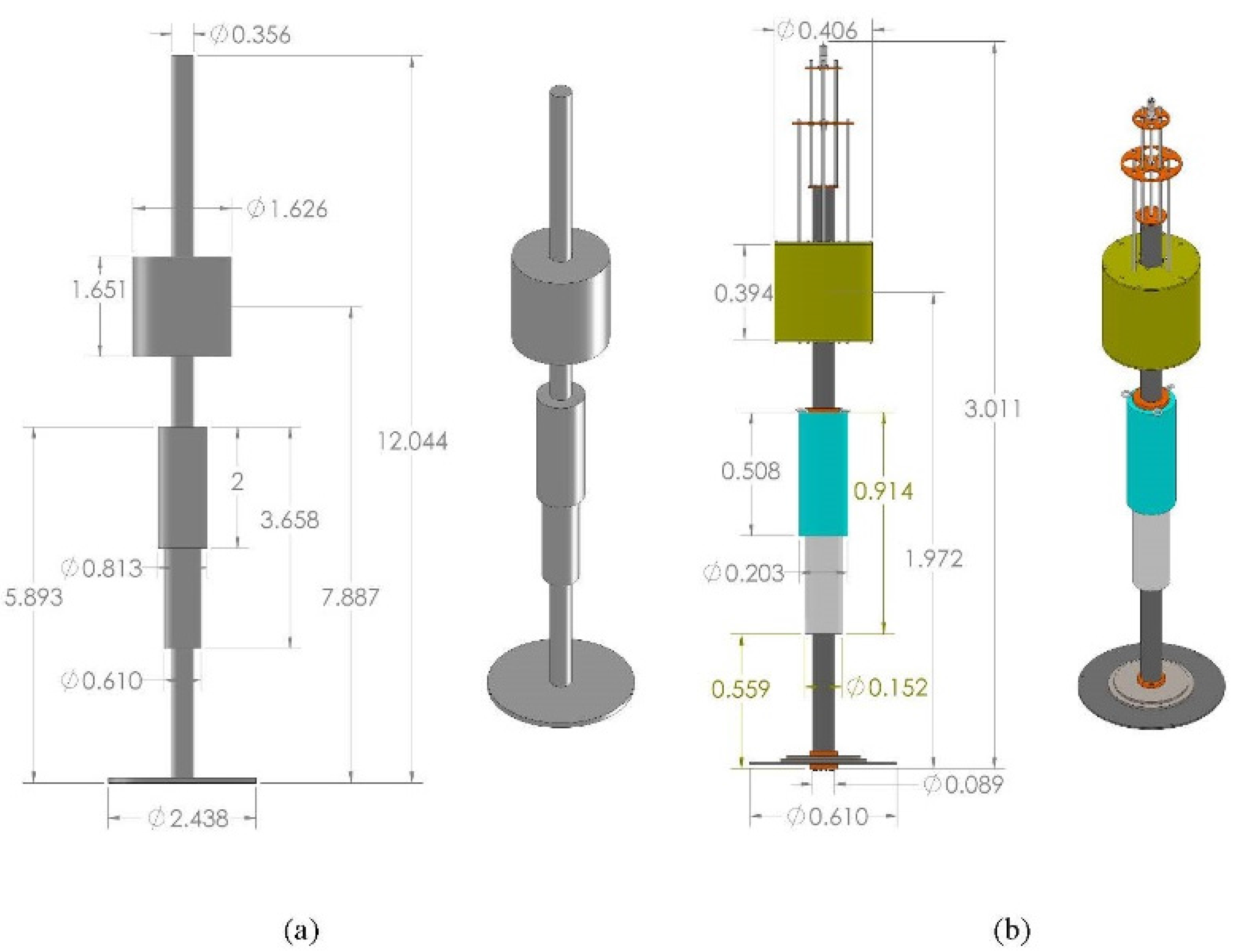
A two-body approach was chosen where the relative motion between the bodies actuates the Power Take Off (PTO). Because of limitations related to the scaled testing facility, the need for additional stability within the system, and the shallow water depth of some prospective sites, a damping plate was added. To add further stability, the metacentric height was raised by the addition of weight to the bottom of the device, and buoyancy was added as high up as possible. This served to lower the center of gravity, while raising the center of buoyancy and thus creating a more stable device. The final-full scale equivalent, and actual fabricated geometry is shown in Figure 1, with the mass properties shown in Table 1.

Figure 1. Autonomous Wave Energy Converter (AWEC): (a) full scale and (b) ¼ scale. All dimensions in meters. The float is toroidal shaped, half submerged in still water, around a central spar body.

Figure 1. Autonomous Wave Energy Converter (AWEC): (a) full scale and (b) ¼ scale. All dimensions in meters. The float is toroidal shaped, half submerged in still water, around a central spar body.

Table 1. AWEC mass properties.

	Full scale		¼ Scale
	Float	Spar	Float	Spar
Mass (kg)	1700	2250	26.5	35.2
Volume (m3)	3.4	2.5	0.053	0.039

Table 1. AWEC mass properties.

	Full scale		¼ Scale
	Float	Spar	Float	Spar
Mass (kg)	1700	2250	26.5	35.2
Volume (m3)	3.4	2.5	0.053	0.039

2.2. Scaling

The prototype built was ¼ the full scale device design. To create the most representative model of the full scale device, with minimal modeling errors due to hydrodynamic and other nonlinear phenomena, the largest scale factor for the prototype was chosen. This was limited by what would reasonably fit in the testing facilities. A near shore location with water depth of about 14 m—a National Oceanic and Atmospheric Administration buoy location off the coast of Galveston, TX—was used as a target location. The maximum water level in the proposed test facility divided by the water depth at the proposed site led to a scaling factor of four. That is to say that in terms of external physical dimensions, the target full scale device would be four times the physical size of the prototype. In scaling the model, ideally, two non-dimensional quantities, the Froude number and the Reynolds number would be held constant. However, for this test, viscous forces are assumed negligible and therefore the Froude scaling is assumed to be valid. Further investigation will inform more detailed viscous force models.

2.3. PTO

The PTO system is responsible for converting the force created by the motion of a WEC to some useful power. As is the case for a heaving point absorber, this often requires the translation of linear motion to rotary motion. There are many ways that this can occur including direct drive solutions as well as intermediate energy conversion solutions such as hydraulic systems. A study of direct drive solutions is performed in [8]. A linear generator system is detailed in [9,10]. For the project documented in this paper, a ball screw spindle drive was chosen coupled to a high efficiency brushed DC motor. At the scale of the built device, this provided the highest efficiency, lowest cost, and easiest implementation with readily available products. For example, one beneficial aspect of this PTO device was the readily available drive electronics consisting of a four quadrant servo-controller. This provided an easily adaptable platform for the implementation of various control schemes [9,10].

2.4. Mooring

The mooring of wave energy conversion devices is very important and should not be overlooked. Mooring can significantly affect the power production, survivability, environmental impact, and cost. An overview of a design approach is given in [11]. Mooring details for the scaled device are shown in Section 4.3. It is anticipated that for full scale open ocean deployment a single point catenary mooring would be favored.

3. Linear Test Bed Testing

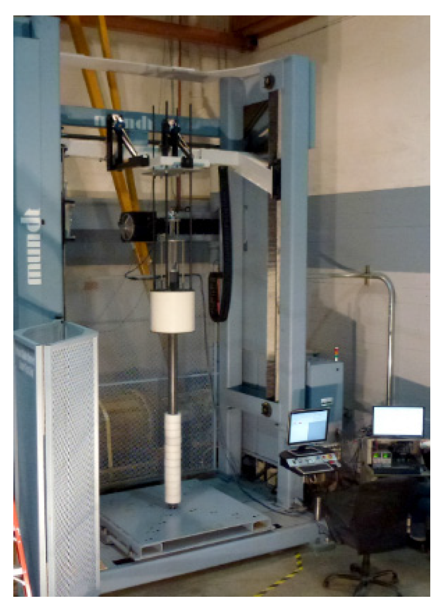
Due to the complex nature of a wave energy converter, there is a lot of useful information that can be gleaned from testing before the device ever enters the water. For this particular project the benefits of dry testing served two purposes. First, it allowed for the testing of most system components in a situation similar to those it sees in the water. Second, it allowed for the characterization of system losses, which are a significant contributing factor affecting the performance of a device. These losses can take many forms, but mostly can be attributed to friction, gearbox, and generator inefficiencies. In an attempt to characterize the system losses, as well as do a complete system validation, a Linear Test Bed (LTB) located in the Wallace Energy Systems and Renewables Facility was used as shown in Figure 2. An overview of the Linear Test Bed is given in [12].

Figure 2. Testing in the Linear Test Bed (LTB). The Linear Test Bed has a maximum stroke of 2 m, force capacity of 20 kN, and a maximum speed of 1 m/s.

Figure 2. Testing in the Linear Test Bed (LTB). The Linear Test Bed has a maximum stroke of 2 m, force capacity of 20 kN, and a maximum speed of 1 m/s.

3.1. Power Delivered to the Load

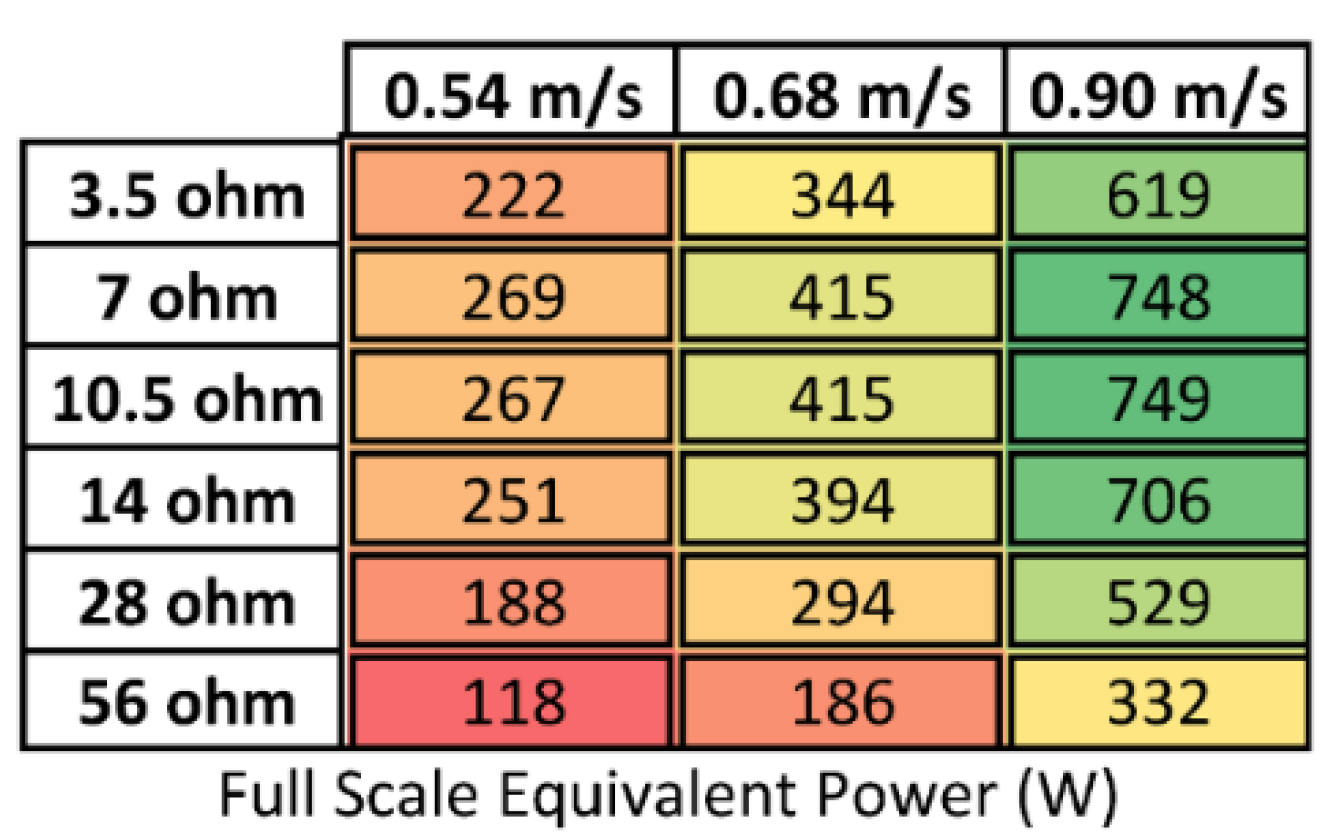
A useful measure of device performance is the electrical power delivered to the load for different operating conditions. A sweep of constant velocities and different load conditions were conducted as trials. Power was measured as the product of the voltage across and current through the DC motor load resistance. This was then scaled using Froude scaling to obtain the full scale equivalent power. DC motors have non-linear characteristics, such as static friction, windage losses, and hysteresis and eddy current losses. These can be included in complex models, but are second order effects and are not included here. Figure 3 shows the results from this test; velocity and power in the table are Froude scaled to full scale.

Figure 3. Power delivered to the load in Watts. Power generally increases as velocity increases. A load resistance near the generator internal resistance (7.41 ohms) provides max power.

Figure 3. Power delivered to the load in Watts. Power generally increases as velocity increases. A load resistance near the generator internal resistance (7.41 ohms) provides max power.

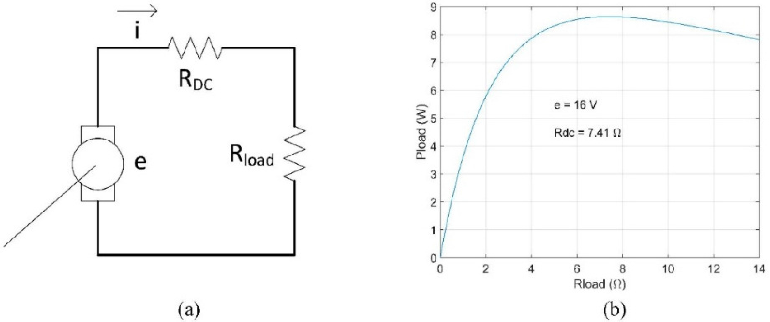
Note that the power generally increases as the velocity increases as expected. Also notice that the load resistance near the internal resistance of the generator (7.41 ohms) provides the max power from the generator. To illustrate this, consider Figure 4 which shows a basic dc motor circuit and power curve. From the maximum power transfer theorem the maximum power transfer occurs when the load resistance matches the internal generator resistance.

Figure 4. (a) Basic DC motor model; (b) Theoretical maximum power transfer between motor and load. Maximum power occurs when the load resistance value is close to the internal motor resistance value.

Figure 4. (a) Basic DC motor model; (b) Theoretical maximum power transfer between motor and load. Maximum power occurs when the load resistance value is close to the internal motor resistance value.

3.2. Loss Modeling

In order to estimate the total losses in the system, a series of tests were conducted. A profile was loaded into the LTB to cause a constant velocity between the float and the spar. For each trial, a velocity and a load condition were chosen, and the power losses were calculated as follows:

$$P_{load}={\left(\frac{e}{R_{DC}+R_{load}}\right)}^2{R}_{load}$$

(1)

$$P_{in}=P_k+P_r+P_{loss}+P_{elec}$$

(2)

$$P_{elec}=V_{gen}{I}_{gen}$$

(3)

where $P_{in}$ is the power input to the system by the LTB; $P_k$ is the rate of change of the linear kinetic energy present in the system which is zero for a constant velocity; $P_r$ is the rate of change of the rotational kinetic energy in the system which is zero for a constant velocity; $P_{loss}$ is the power losses in the system, and $P_{elec}$ is the power measured out of the generator.

$$P_{loss}=P_{in}-P_{elec}$$

(4)

The power input to the system $P_{in}$ was measured as the force (measured with load cells) imparted on the device under test multiplied by the velocity.

$$P_{in}=F_{in}v$$

(5)

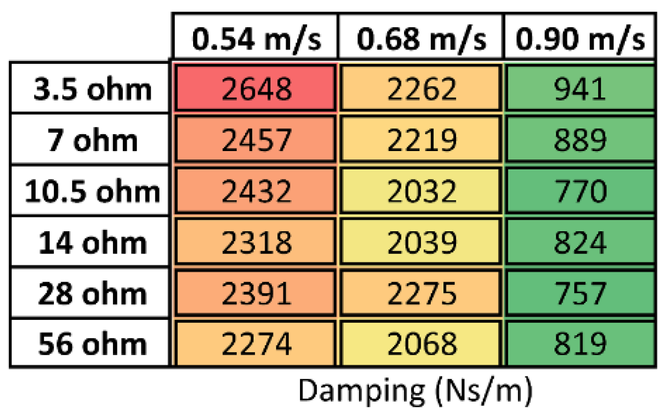
In order to include the losses in any model of the overall system, an estimate of those losses should be included. Although these losses are nonlinear, a linear damping term is a simple way to implement the estimated losses and is a good first pass approximation as shown in Chapter 13 in [13] and Section 2.3 in [14]. This term can be estimated as follows:

$$F_{loss}=B_{loss}v$$

(6)

$$P_{loss}=F_{loss}v=B_{loss}{v}^2$$

(7)

$$B_{loss}=\frac{P_{loss}}{v^2}$$

(8)

where $F_{loss}$ is the equivalent loss force in the system; $B_{loss}$ is the loss damping and captures friction and other high order loss mechanisms; v is the linear velocity; and $P_{loss}$ is the power lost due to the inefficiencies of the system. Again, the velocity and load conditions were swept with the resulting estimates for $B_{loss}$ shown in Figure 5; velocity and power in the table are Froude scaled to full scale. As expected, the higher speeds produced a lower estimated damping value. Based on these results, and anticipated tank testing velocities from 0.1 m/s to 0.7 m/s, a mean value of 2000 Ns/m was used in both AQWA and MATLAB/Simulink full scale models.

Figure 5. Estimated loss damping values for a sweep of velocity and load values. Higher speeds produced lower estimated damping values.

Figure 5. Estimated loss damping values for a sweep of velocity and load values. Higher speeds produced lower estimated damping values.

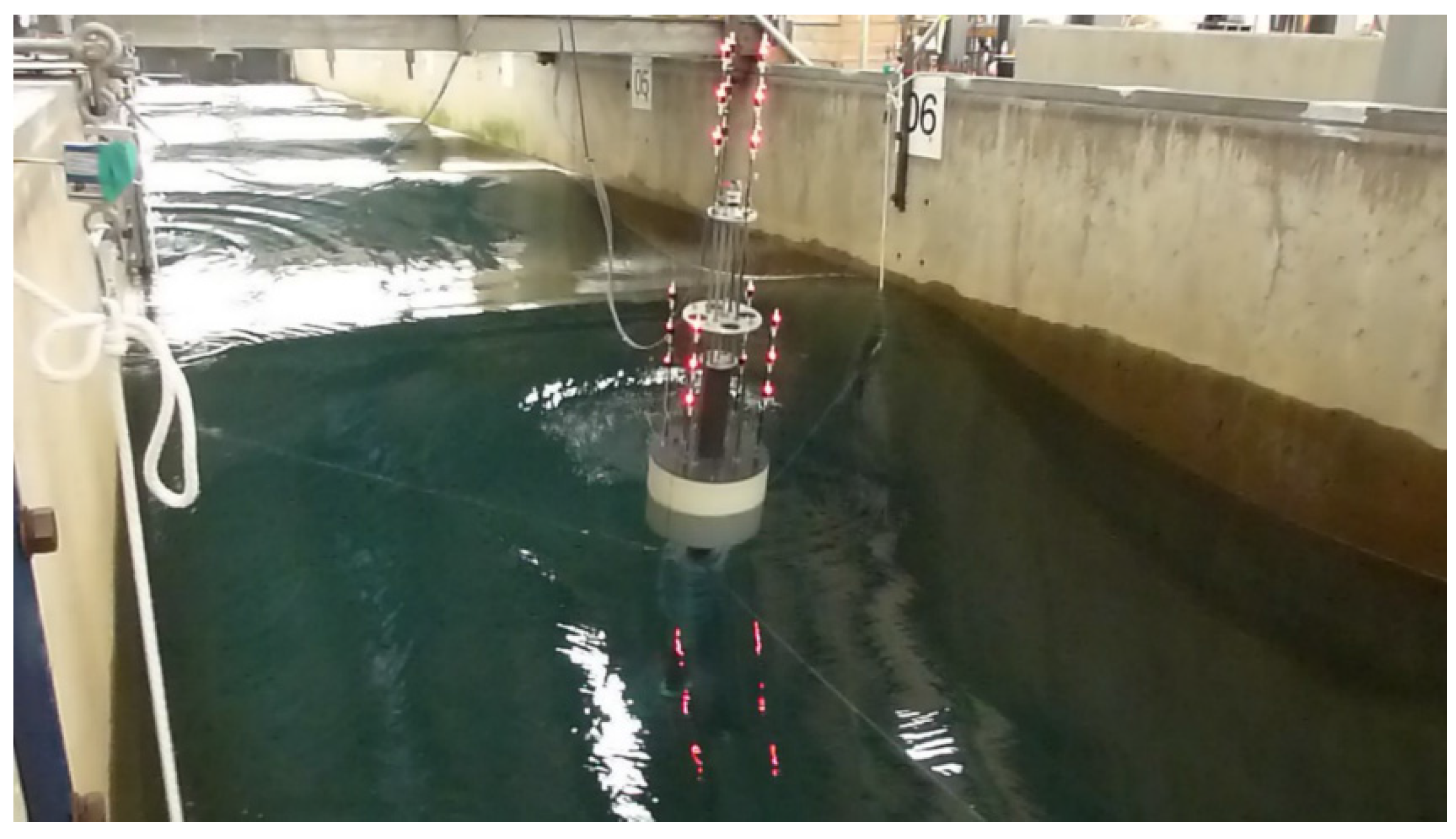
4. Wave Tank Testing Facilities

The next step in the model validation process was testing the scaled AWEC model in the large wave flume located in the O.H. Hinsdale Wave Research Laboratory (HWRL) at Oregon State University (OSU). The HWRL has performed similar wave energy converter testing in the large wave flume as detailed in [15], and shown in Figure 6, which made for a relatively smooth process for testing. Data from the test trials were recorded for the three major data acquisition systems included in the testing. This included the wave flume, optical tracking, and device performance data which will be reviewed in the following sections.

4.1. Large Wave Flume

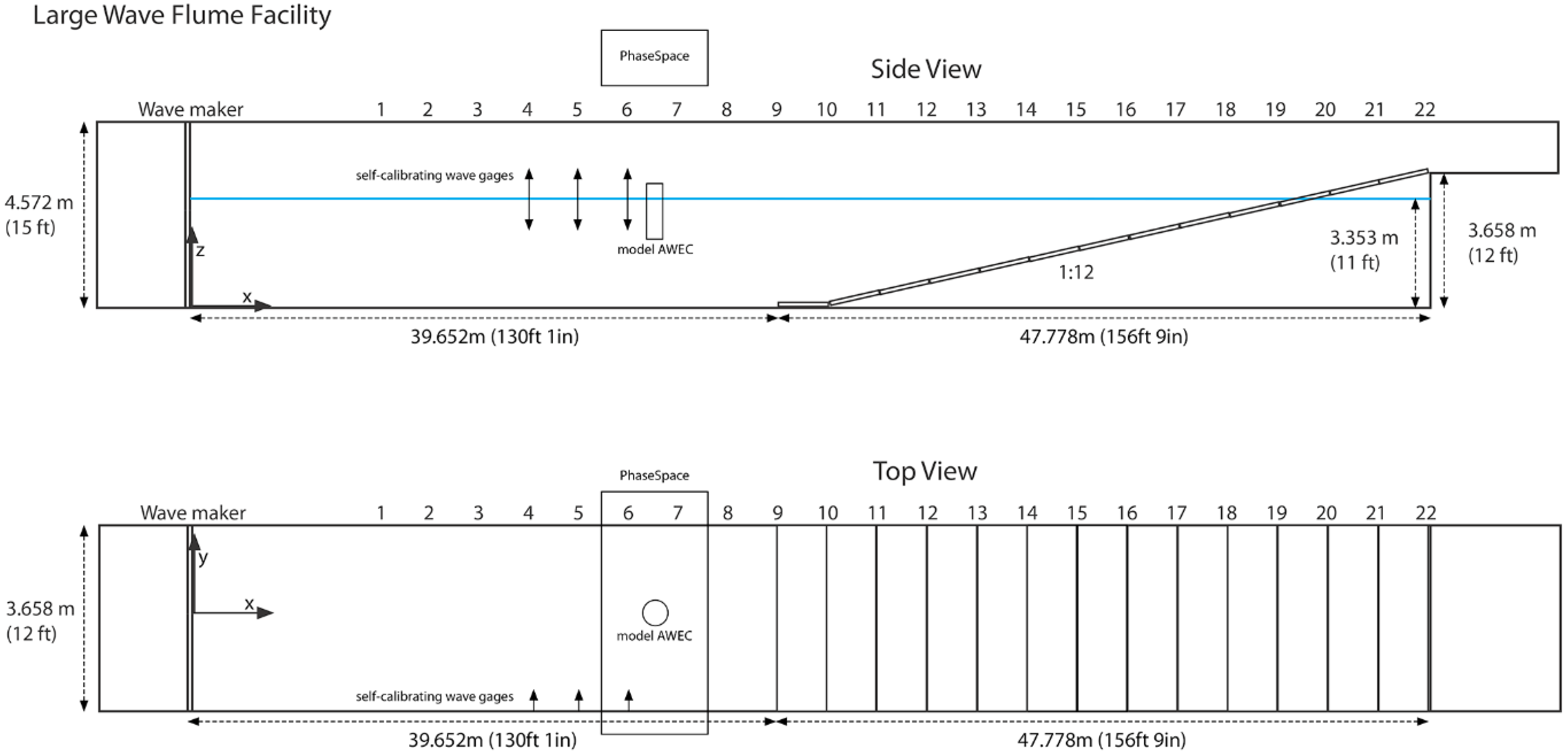
The large wave flume is one of the largest of its kind in North America and measures 88 m long by 3.7 m wide and 4.6 m deep. The wave maker is hydraulic-piston actuated, and capable of creating regular, irregular, tsunami, and user-defined wave types. The period range is from 0.5 to 10 s with a maximum wave height of 1.6 m at a 7-second period. A 1:12 slope concrete beach was selected to minimize reflections within the tank. A water depth of 3.353 m was chosen as this was the maximum reasonable depth for testing in the flume.

For the AWEC testing setup, several data acquisition measurements related to the wave tank were included. A wavemaker start signal, wavemaker displacement, a wavegauge located at the wavemaker, and a pressure sensor level signal were all recorded. Additionally, three resistance-type self-calibrating wave gauges offset from the tank wall near the device under test were recorded. All signals were logged with a data acquisition system with a sampling rate of 50 Hz. Figure 6 shows the basic geometry and layout of the large wave flume, with the location of the wave gauges, device under test (model AWEC), and optical tracking system (PhaseSpace).

Figure 6. Large wave flume configuration.

Figure 6. Large wave flume configuration.

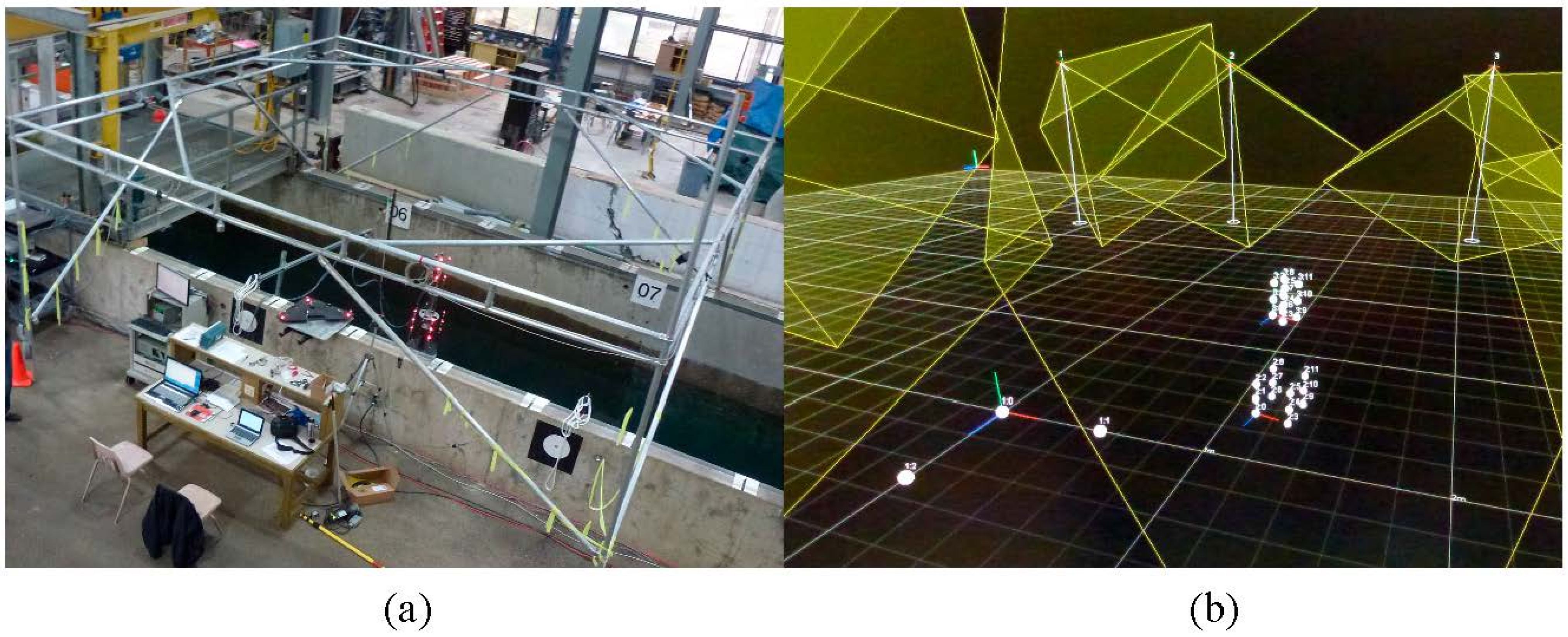
4.2. Optical Motion Capture System

In attempting to validate numerical models of the AWEC system, it was very important to have confidence in the motion tracking data of the bodies under test. A PhaseSpace optical motion capture system was used for this purpose. This system, designed for the entertainment industry, allows high resolution tracking of rigid bodies. Twenty-seven uniquely identified active LED markers viewed by eight cameras surrounding the device describe the PhaseSpace setup. Motion data is recorded at a 480 Hz sampling rate. Previous tests found a 6-sigma accuracy of 0.9 mm for all targets within a 1.2 m radius, and 1.3 mm accuracy up to a 2.5 m radius [15]. Each body of the AWEC was uniquely identified for six degrees of freedom in relation to the reference coordinate definition square. Figure 7 shows the PhaseSpace setup on the left and a computer image showing the cameras and markers for each LED on the right.

Figure 7. Optical motion tracking: (a) Setup in the O.H. Hinsdale Wave Research Laboratory (HWRL); and (b) screen capture of tracking markers.

Figure 7. Optical motion tracking: (a) Setup in the O.H. Hinsdale Wave Research Laboratory (HWRL); and (b) screen capture of tracking markers.

4.3. Mooring

For testing in the large wave flume at the HWRL, a three point mooring system was constructed and implemented. Each line was installed in pretension in a horizontal plane with a 120° angle between the lines. The aft mooring line was parallel to the wave tank walls. Each line had a pulley system which led to a load cell on the edge of the tank. Mooring force was recorded for each line. Each line consisted of a 1.5 m un-stretched length of surgical tubing and a length of stiff rope. Experimental testing on the surgical tubing revealed an estimated stiffness of 520 N/m for a full scale equivalent, obtained using Froude scaling. Each line was set in a pretension of 260 N full scale equivalent (i.e., pre-stretched 0.5 m). The surgical tubing was tested before connecting the mooring system and the stiffness was found to be suitably linear over the range of expected tensions. Assuming the x-y plane to be collinear with the three point mooring forces, i.e., surge and sway, and the z-axis to be heave, the linearized stiffness about the equilibrium point is 780 N/m in x and y directions and 0 N/m in the z direction. Thus this mooring design will hold the model centered in the tank, yet not restrict the desired heave motion.

4.4. Device Performance Data

Device performance data from the AWEC was also recorded with the data acquisition system. In all, sixteen channels of data were recorded at a 50 Hz sampling rate using the HWRL data acquisition system. The signals can be broken into two categories, namely signals related to the PTO and signals related to the mooring.

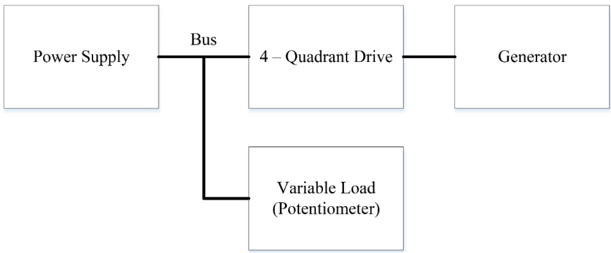
Several signals related to the PTO, consisting of a lead screw, gearbox, generator, and encoder were logged. From the encoder data, position, velocity, and acceleration signals were recorded, which describe the relative motion between the two bodies: the float and spar. Voltages and currents were logged including the system bus voltage, power supply current, and load current. The general setup for the PTO circuit is shown in Figure 8. Several signals related to the 4-quadrant drive were logged including the drive current, drive velocity, commanded current, and the enable command. Additionally each of the three mooring lines had a load cell attached, and this mooring force was also recorded.

Figure 8. Power Take Off circuit.

Figure 8. Power Take Off circuit.

5. Wave Tank Testing Procedure

Wave tank testing occurred over a two week period in the HWRL. Three and a half days were dedicated to the setup of the wave tank. This included installation of the mooring system, installation of the device under test, installation of the optical motion tracking system, installation of the wave gauges and related wave tank systems, filling of the tank, and calibration of the system. Six days were then dedicated to experimental testing which is outlined below. Figure 9 shows the device under test.

Figure 9. AWEC testing in the Hinsdale Wave Research Laboratory at Oregon State University.

Figure 9. AWEC testing in the Hinsdale Wave Research Laboratory at Oregon State University.

5.1. Experimental Methodology and Procedure

Each individual running of waves was considered to be a trial. Each trial was a member of an experiment. In all, there were nine experiments conducted with a total of one hundred and forty-three trials. All trials were run with either monochromatic or Pierson-Moskowitz spectral wave input. In general, with a few exceptions, the length of run was set to 200 waves (based on the peak period if spectral). In addition to the 200 waves, there was a ramp up time and ramp down time associated with the data acquisition and the wavemaker. Also in general, if control was to be implemented in the run, which was the case for most trials, the first ten percent of the trial was run with the control off. At ten percent of the total trial length the control was then activated and applied for the duration of the trial. This provided a baseline operation for each trial to see the effects of control on the system.

5.2. Types of Trials Conducted

Of the hundred and forty-three trials conducted throughout the testing, the bulk of the trials fit into four experiments. In an attempt to characterize the device, a sweep of wave height and period was conducted with a monochromatic input creating a five by five matrix. Also in characterizing the device, a sweep of irregular waves was performed, sweeping significant wave height and dominant wave period for a similar five by five matrix of values. The final experiments were conducted as an exercise in testing a binary and tertiary control scheme for generating more power from the AWEC. The results of these last two experiments will be published separately.

6. Results

The main thrust of this work involved the model validation of a scaled prototype using numerical modeling techniques. Two numerical modeling tools, ANSYS AQWA and MATLAB/Simulink, were used to run full scale equivalent models of the AWEC. Results from the tank testing were scaled up for comparison with the numerical results using Froude scaling. Because of the discrepancies between the commanded and measured wave heights and periods, input to the numerical models were made to match full scale equivalent measured wave tank wave heights and periods.

6.1. Commanded vs. Measured Wave Tank Results

For regular wave inputs wave gauge readings were taken on the wave maker side of the AWEC. A desired period and wave height was given to the wave maker operator for each trial. The resulting wave surface elevation was recorded at the location of the wave gauge closest to the AWEC. All wave gauge data was filtered using a fourth order bandpass Butterworth filter with a passband between 0.1 Hz and 3 Hz. The resulting measurement of the wave period closely matched the expected period, however, the measured wave height deviated from the expected by as much as 29%. Furthermore, for different periods given the same expected wave height, the measured average wave height varied. Because of these results, all time domain simulations done in both AQWA and MATLAB/Simulink received the scaled measured input wave height in order to compare the theoretical results to measured results.

For irregular wave input, a similar process was followed. Because of restrictions on the operation of the wave maker, two of the trials in the matrix were unable to be completed. Results showed that there is significant error in both peak period and significant wave height with a max error of 27% and 35% respectively. In order to compare the hardware results with the numerical modeling, a scaled time series of measured wave heights was used as the input to the AQWA and MATLAB/Simulink numerical modeler.

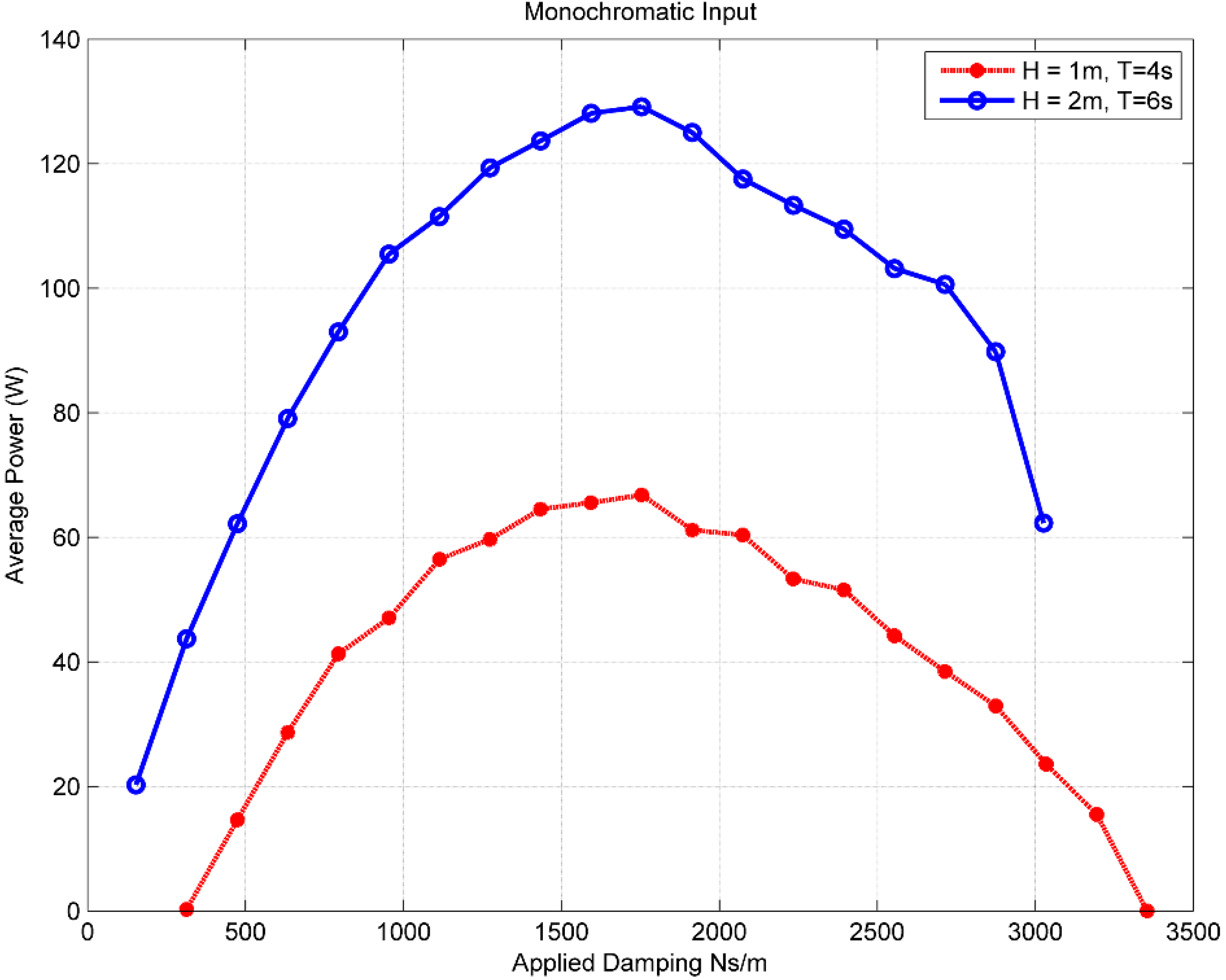
6.2. Max Damping Value

For purposes of model validation and characterization of the system a fixed damping value was needed in order to conduct the tests. In order to achieve a fixed damping value the 4-quadrant drive was set in a current control (i.e., torque control) operating mode. A velocity proportional damping term B (Ns/m) was then used to set the desired torque command to the motor. Early tests were run using a monochromatic wave input to the system. As the trial progressed, after approximately every ten waves the damping values were stepped up. Figure 10 shows the results from a damping sweep for two different monochromatic input waves, one with a full scale wave height of 1 m and period of 4 s, and one with a full scale wave height of 2 m and period of 6 s.

Figure 10. Average Power vs. Damping for two monochromatic wave inputs.

Figure 10. Average Power vs. Damping for two monochromatic wave inputs.

As the plot shows, the maximum full scale damping value for either case was near B = 1600 Ns/m, which was then chosen as the base damping value to be used for all sweeps of wave height and period, both monochromatic and spectral.

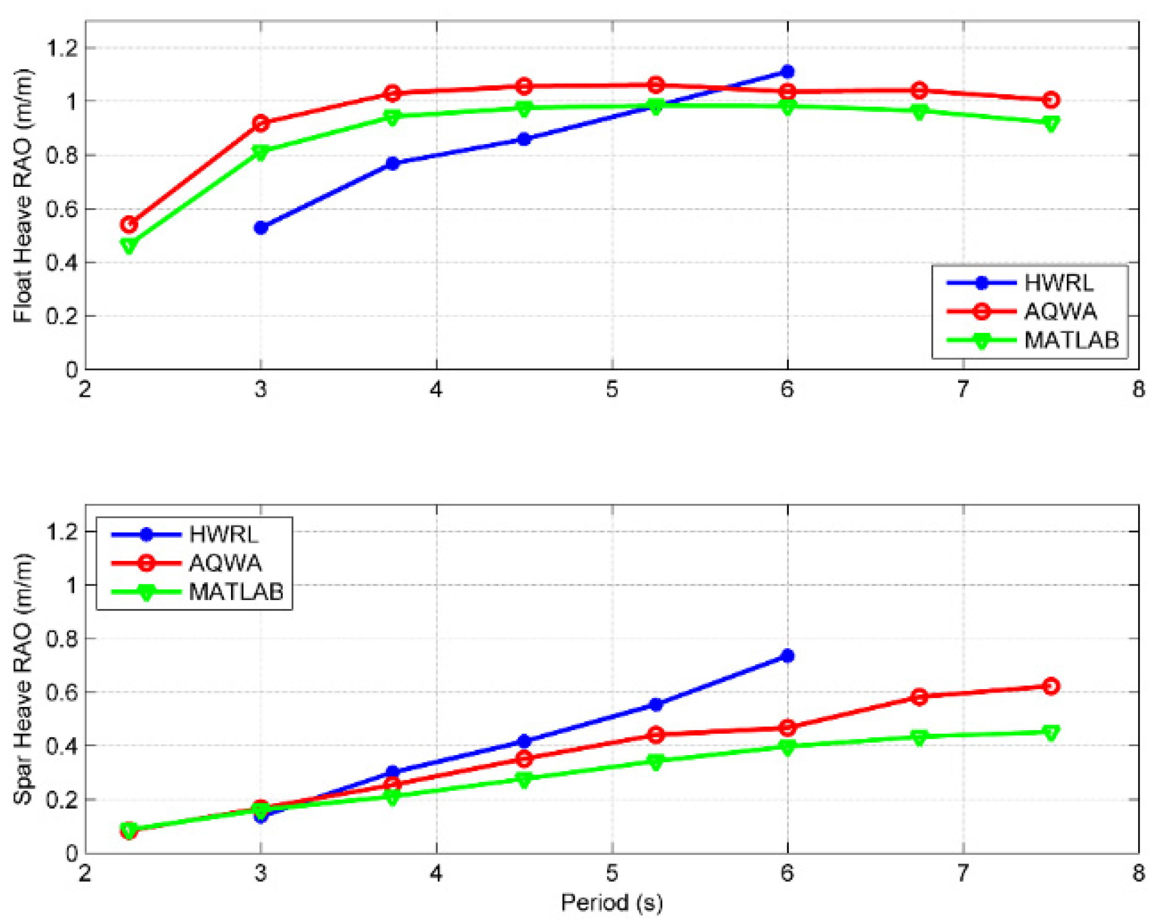
6.3. Response Amplitude Operators (RAOs)

Testing in regular waves gives insight into the behavior of the system in a relatively controlled environment, controlled by two parameters namely wave height and wave period. One measure of the performance of such regular wave tests is the calculation of the Response Amplitude Operator (RAO). The RAO is essentially a transfer function describing the relationship between an input and output characteristic of the components of the device of interest. Traditionally, in ship design, RAOs are often used in the design stage to determine modifications that may need to occur for safety reasons. In ocean wave energy conversion RAOs can be useful in design for maximum power extraction. For this study, because of the nature of the point absorber, the heave motion was identified as the pertinent motion for energy capture and thus the RAO was calculated for each body, namely the float heave and spar heave as follows:

$$RAO=\frac{\zeta }{\eta }\left[\frac{m}{m}\right]$$

(9)

where ζ is the body heave amplitude and η is the incoming wave amplitude. For each body the time series response was analyzed to find the positive zero crossings. Then for each period the amplitude of the waveform was calculated. The average of these values was then determined to be the body average heave amplitude. A similar process was used to obtain the average incoming wave amplitude.

As part of the model validation process, three sets of heave RAOs were calculated and compared for each rigid body. First, the tank test results of wave surface elevation as measured by the resistance wave gauges was used with the optical motion tracking information from PhaseSpace for the heave amplitude of each body. Second, time domain simulations from six degrees of freedom ANSYS AQWA-NAUT were used to calculate the heave RAO. Third, a heave-only time domain model was implemented in MATLAB/Simulink, based on the frequency domain parameters obtained from ANSYS AQWA LINE. The methodology and a review of this modeling process is outlined in [16]. The heave motion RAOs for the three data sets are shown in Figure 11. Results show the float acts close to a wave follower, that is to say, for a certain input wave height the response is close to the same in magnitude. Conversely, the response of the spar is greatly attenuated from the input waveform, causing relative motion between the two bodies, which is the mode for electricity generation. The AQWA and MATLAB results are in reasonable agreement and generally have the same shape with regard to frequency. However, both AQWA and MATLAB appear to be missing some high frequency behavior for the float and low frequency behavior for the spar present in the tank testing results. In the case of the float, wave steepness, which is higher at higher frequencies, may cause more nonlinear behavior and help explain the divergence in the results. Additionally, any unmodelled viscous forces, which are proportional to the square of speed, will be more significant. For the spar, the low frequency behavior could be accounted for by longitudinal resonant modes of the wave flume, which are not included in the AQWA and MATLAB models. The cause for the discrepancy will be investigated in future research.

Figure 11. Response Amplitude Operators (RAOs) for HWRL, AQWA, and MATLAB. The PTO damping is set to 1600 Ns/m as described in Section 6.2.

Figure 11. Response Amplitude Operators (RAOs) for HWRL, AQWA, and MATLAB. The PTO damping is set to 1600 Ns/m as described in Section 6.2.

6.4. Power Characteristics

One key measure of the performance of a wave energy converter is its average power output. This is particularly important for an autonomous application because a sensor package may rely on a certain baseline average power production for consumption. In characterizing a device it is most useful to look at the power output for irregular waves because this will be the case for any real world conditions. As outlined earlier, a sweep of significant wave height and peak period was done to create a 5 × 5 matrix of system outputs. Power production was calculated by measuring the bus voltage and the currents in the circuit and then calculating the power generated by the PTO. The result is the total power produced including all losses. 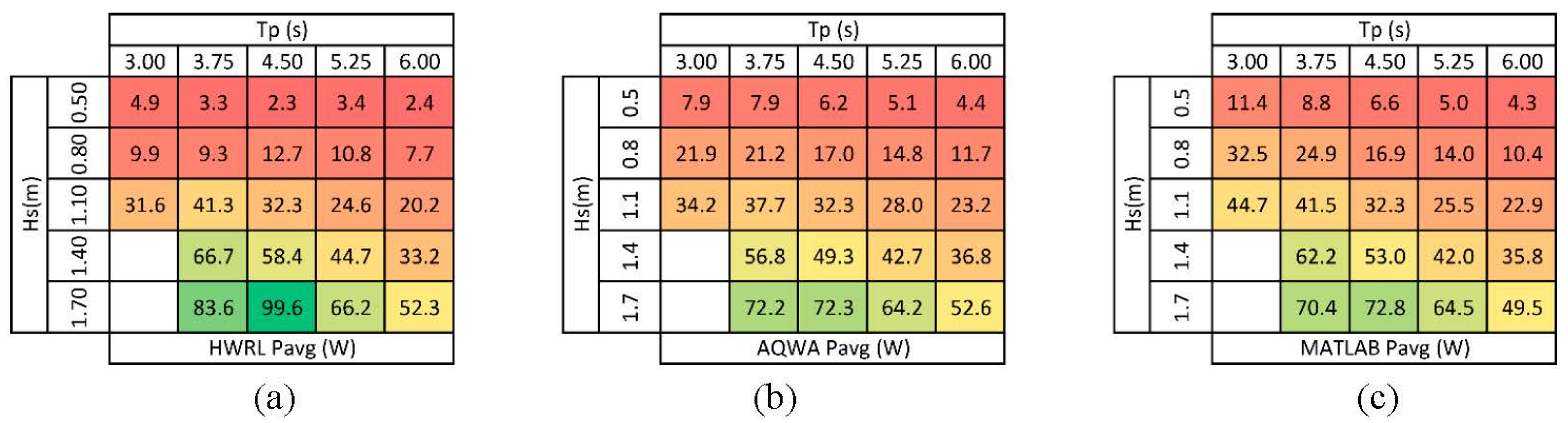Time domain simulations were then performed using ANSYS AQWA-NAUT and a time domain simulation tool in MATLAB/Simulink developed by the author, described in [17], in an attempt to simulate the testing environment. As described earlier, the losses implemented in the numerical models were estimated as additional damping in the system. The result is a power matrix plot showing the average power output for different combinations of significant wave height and peak period irregular wave inputs for one experimental test and two hydrodynamic modeling exercises as shown in Figure 12.

Figure 12. Power Matrix for irregular wave input: (a) HWRL wave tank testing; (b) AQWA model; and (c) MATLAB model. All quantities are Froude scaled to full scale.

Figure 12. Power Matrix for irregular wave input: (a) HWRL wave tank testing; (b) AQWA model; and (c) MATLAB model. All quantities are Froude scaled to full scale.

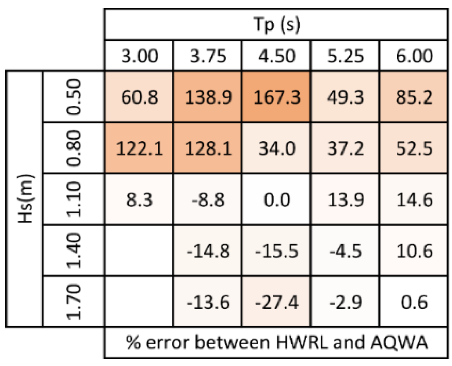
In order to quantify the differences between the model and the measured data, the percent error was calculated between the different methods. Figure 13 shows the % error between the measured data and AQWA simulated data. As shown, the match is quite good at the nominal case. As lower significant wave heights and peak periods are analyzed the error generally gets larger, with the AQWA model over-predicting the power output of the system. As significant wave heights increase and peak periods decrease the trend shows an AQWA under-prediction of power output. This may be due to nonlinear PTO characteristics such as friction which may be more dominant at the lower significant wave heights and lower WEC speeds. These effects were not included in the numerical model as a constant linear damping term was used.

Figure 13. Percent error between measured tank testing data and AQWA model data. AQWA over-predicts for lower significant wave heights and peak periods. AQWA under-predicts for higher significant wave heights and peak periods. All quantities are Froude scaled to full scale.

Figure 13. Percent error between measured tank testing data and AQWA model data. AQWA over-predicts for lower significant wave heights and peak periods. AQWA under-predicts for higher significant wave heights and peak periods. All quantities are Froude scaled to full scale.

7. Conclusions

This work provides an overview of linear test bed and wave tank testing procedures, as well as model validations stemming from the tank testing results. Design and testing methodologies were overviewed and results for characterizing a WEC and validating a model were given. Results include power output results from irregular wave input, and response amplitude operator (RAO) results from regular wave input. Numerical methods were shown to have relatively accurate results around a nominal operating point with increased error in the model as the conditions varied from the nominal. Tank testing of the AWEC showed under sufficiently energetic wave conditions electrical power generation performance met the target. Future work includes refinements to the hydrodynamic design and the PTO system to improve power generation under more nominal conditions.

References

- Holmes, B. Tank Testing of Wave Energy Conversion Systems. European Marine Energy Centre (EMEC): Orkney, UK. Available online: http://www.emec.org.uk/tank-testing-of-wave-energy-conversion-systems/ (accessed on 3 December 2012).
- Payne, G.; Ingram, D. Best practice guidelines for tank testing of wave energy converters. J. Ocean Technol. 2009, 4, 38–70. [Google Scholar]
- High Level EquiMar Protocols—EquiMar. Available online: http://www.equimar.org/high-level-equimar-protocols-.html (accessed on 1 November 2013).
- Cruz, J. Ocean Wave Energy: Current Status and Future Prespectives, 1st ed.; Springer: Berlin, Germany, 2008. [Google Scholar]
- Hart, P. Autonomous Powerbuoys: Wave Energy Converters as Power Sources for the Next Generation of Ocean Observatories. Available online: http://virtual.ocean-news.com/article/Autonomous_Powerbuoys%3A_Wave_Energy_Converters_As_Power_Sources_For_The_Next_Generation_Of_Ocean_Observatories/1081385/114319/article.html (accessed on 9 May 2013).
- Falcão, A.F.O. Wave energy utilization: A review of the technologies. Renew. Sustain. Energy Rev. 2010, 14, 899–918. [Google Scholar] [CrossRef]
- Lewis, T.M.; von Jouanne, A.; Brekken, T.K.A. Modeling and control of a slack-moored two-body wave energy converter with finite element analysis. In Proceedings of the 2012 IEEE Energy Conversion Congress and Exposition (ECCE), Raleigh, NC, USA, 15–20 September 2012; pp. 938–945.
- Rhinefrank, K.; Schacher, A.; Prudell, J.; Brekken, T.K.A.; Stillinger, C.; Yen, J.Z.; Ernst, S.G.; von Jouanne, A.; Amon, E.; Paasch, R.; et al. Comparison of Direct-Drive Power Takeoff Systems for Ocean Wave Energy Applications. IEEE J. Ocean. Eng. 2012, 37, 35–44. [Google Scholar] [CrossRef]
- Bostrom, C.; Waters, R.; Lejerskog, E.; Svensson, O.; Stalberg, M.; Stromstedt, E.; Leijon, M. Study of a Wave Energy Converter Connected to a Nonlinear Load. IEEE J. Ocean. Eng. 2009, 34, 123–127. [Google Scholar] [CrossRef]
- Bostrom, C.; Ekergard, B.; Waters, R.; Eriksson, M.; Leijon, M. Linear Generator Connected to a Resonance-Rectifier Circuit. IEEE J. Ocean. Eng. 2013, 38, 255–262. [Google Scholar] [CrossRef]
- Johanning, L.; Smith, G.H.; Wolfram, J. Mooring design approach for wave energy converters. J. Eng. Marit. Environ. 2006, 220, 159–174. [Google Scholar] [CrossRef]
- Hogan, P.M. A Linear Test Bed for Characterizing the Performance of Ocean Wave Energy Converters. Master’s Thesis, Oregon State University, Corvallis, OR, USA, 2007. [Google Scholar]
- Mohan, N.; Robbins, W.P.; Undeland, T. Power Electronics; John Wiley & Sons: Hoboken, NJ, USA, 1995. [Google Scholar]
- Krause, P.C.; Wasynczuk, O.; Sudhoff, S.D.; Pekarek, S. Analysis of Electric Machinery and Drive Systems; John Wiley & Sons: Hoboken, NJ, USA, 2013. [Google Scholar]
- Rhinefrank, K.; Schacher, A.; Prudell, J.; Hammagren, E.; Stillinger, C.; Naviaux, D.; Brekken, T.; von Jouanne, A. Scaled wave energy device performance evaluation through high resolution wave tank testing. In Proceedings of the OCEANS 2010, Seattle, WA, USA, 20–23 September 2010; pp. 1–6.
- Bosma, B.; Zhang, Z.; Brekken, T.K.A.; Ozkan-Haller, H.T.; McNatt, C.; Yim, S.C. Wave energy converter modeling in the frequency domain: A design guide. In Proceedings of the 2012 IEEE Energy Conversion Congress and Exposition (ECCE), Raleigh, NC, USA, 15–20 September 2012; pp. 2099–2106.
- Bosma, B.; Brekken, T.; Ozkan-Haller, H.T.; Yim, S.C. Wave Energy Converter Modeling in the Time Domain: A Design Guide. In Proceedings of the IEEE Conference on Technologies for Sustainability, Portland, OR, USA, 1–2 August 2013; pp. 103–108.
© 2015 by the authors; licensee MDPI, Basel, Switzerland. This article is an open access article distributed under the terms and conditions of the Creative Commons Attribution license (http://creativecommons.org/licenses/by/4.0/).