A Novel Grouping Method for Lithium Iron Phosphate Batteries Based on a Fractional Joint Kalman Filter and a New Modified K-Means Clustering Algorithm

Abstract

This paper presents a novel grouping method for lithium iron phosphate batteries. In this method, a simplified electrochemical impedance spectroscopy (EIS) model is utilized to describe the battery characteristics. Dynamic stress test (DST) and fractional joint Kalman filter (FJKF) are used to extract battery model parameters. In order to realize equal-number grouping of batteries, a new modified K-means clustering algorithm is proposed. Two rules are designed to equalize the numbers of elements in each group and exchange samples among groups. In this paper, the principles of battery model selection, physical meaning and identification method of model parameters, data preprocessing and equal-number clustering method for battery grouping are comprehensively described. Additionally, experiments for battery grouping and method validation are designed. This method is meaningful to application involving the grouping of fresh batteries for electric vehicles (EVs) and screening of aged batteries for recycling.

1. Introduction

With the development of EVs, battery technology has drawn more and more attention worldwide. Battery packs are core components of EVs; they are composed of hundreds or thousands of small cells joined by series-parallel connections. Owing to the subtle differences in the battery production process, the electric characteristics of the batteries are slightly different. The current flowing through the batteries will thus be inconsistent and the temperature inside the battery pack will be uneven when the inconsistent batteries are connected in parallel. In this case, battery use will accelerate their decay and some safety problems will occur [1]. In series connection, the potential of most batteries in the battery pack will not exhaust. Moreover, battery state monitoring and management, such as state of charge (SoC), state of health (SoH) estimation [2,3,4] and state of peak power (SoP) prediction [5,6], will become more and more difficult. Therefore, measures are necessary to guarantee the characteristics of the grouped batteries are as similar as possible.

Numerous battery grouping methods have been reported in previous studies. Kim et al. proposed a battery voltage and SoC consistency screening method based on matching battery DC resistance [7,8]. Schneider et al. used a sorting method for aged batteries [9]. In that paper, the sorting steps for these batteries are designed. Fang et al. proposed a method for battery classification based on the thermal behavior during the charging process [10]. In the method, differences in battery surface temperature are used to evaluate the consistency of batteries. At present, battery capacity, AC resistance, electrochemical impedance spectroscopy (EIS), voltage curve, battery model parameter, charge and discharge thermal behavior are the commonly used parameters to evaluate consistency.

In the authors’ previous work [11], the reliability and effectiveness of these evaluation bases are comprehensively analyzed. The main arguments are summarized as follows: AC resistance represents only a small part of the impedance characteristics of the battery, and this parameter cannot reflect the dynamic characteristics of the battery, since the testing frequency (about 1 kHz) is much higher than the main frequency component of the driving conditions. Battery charge and discharge voltage curves can reflect the voltage consistency under the test conditions, however, the reliability of any conformance assessment will be decreased if the working conditions change. Additionally, the voltage curve is just an external manifestation of the battery, and the internal characteristics’ consistency cannot be guaranteed because of the complex relationship between voltage curve and internal material properties. The surface temperature of a battery is determined by the entropy heat, resistance heat and surface heat dissipation. The parameters can reflect the battery performance, but they are susceptible to the external environment. EIS or battery model parameters can better reflect the dynamic characteristics of a battery. Capacity consistence determines that the performance of batteries in the battery pack cannot reach their full potential. However, battery capacity is obtained by constant current charge and discharge tests, EIS is measured by sweep frequency impedance tests and battery model parameters are obtained by intermittent constant current and pulse current tests. Considerable time and special testing instruments are required for these three tests.

The existing battery clustering algorithms include the self-organizing feature map algorithm (SOM) [10], fuzzy c-means (FCM) clustering algorithm, etc. [12,13,14]. These earlier works focus more on the similarity of batteries’ characteristics. However, the number of elements in each group after grouping is different and not equal to the design number of batteries in each pack.

After review of the problems of the battery consistency evaluation parameter extraction methods and battery clustering algorithms, this paper presents a novel battery grouping method. This method can be divided into two parts: the first part is the battery characteristic parameter extraction, which is based on a simplified EIS model, fractional joint Kalman filter algorithm and DST—the details are described in Section 2. The second part is a new modified K-means clustering algorithm especially proposed for battery equal-number grouping—this part are presented in Section 3. The proposed method is established based on a short time charge and discharge experiment. The characteristic parameters including open circuit voltage (OCV), simplified EIS model parameters and battery capacity can be obtained. All these parameters have relatively clear physical meanings. The clustering algorithm can divide the batteries into equal-number groups according to the similarity of consistent evaluation parameters and the number of elements designed by engineers in each group.

2. Battery Parameter Extraction

2.1. Battery Model Selection

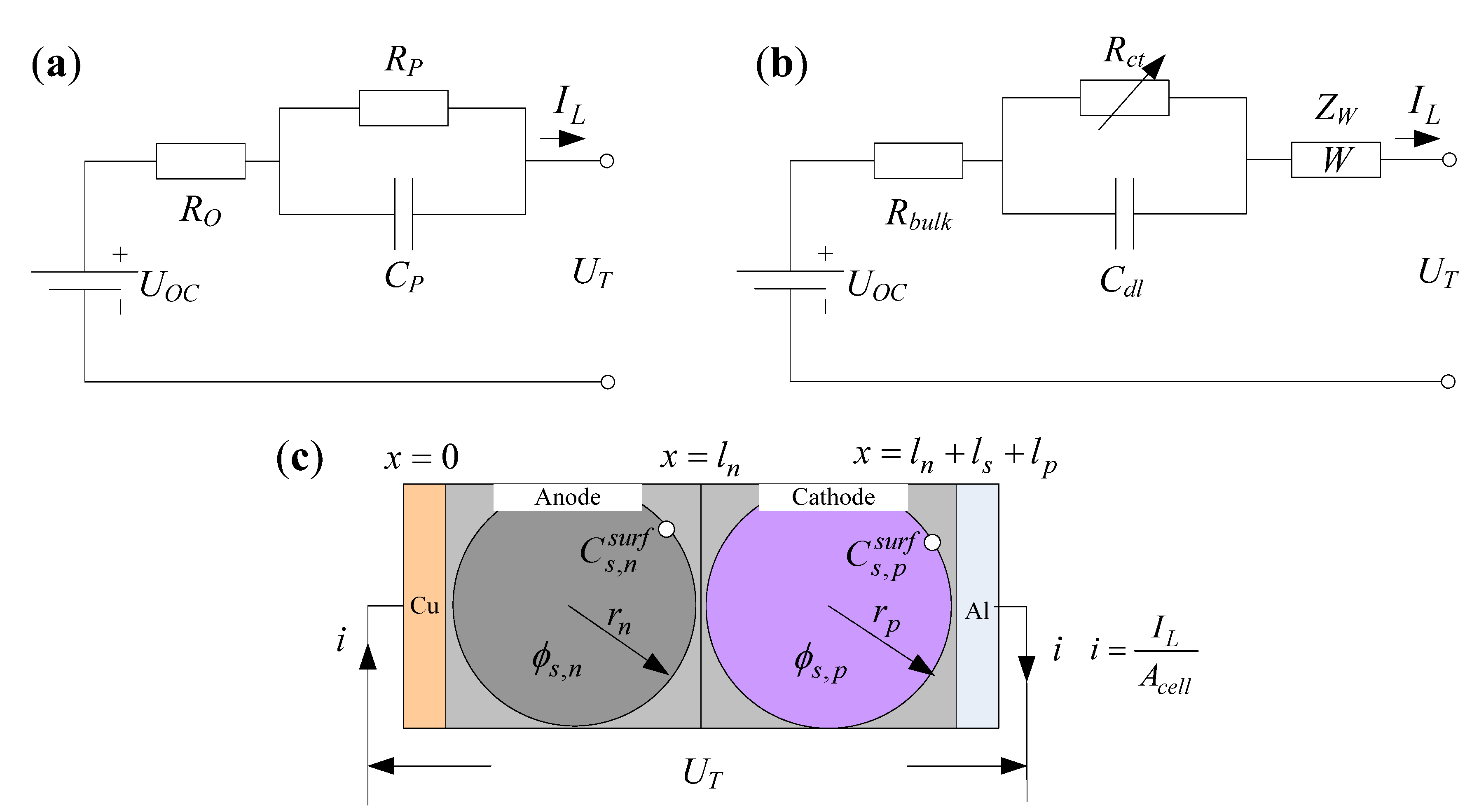
2.1.1. Comparison of Battery Models

It is essential to select a suitable model for quantifying battery characteristics. Recent battery models mainly involve equivalent circuit models based on the external electric characteristics of battery charge and discharge (ECMs for short in this paper) or electrochemical impedance spectroscopy tests (EIS models), electrochemical reaction mechanism models (ERM models), etc. In ECMs, resistance, capacitor and diodes are commonly used. Their structures are simple and easy to calculate. These models are widely used in battery state monitoring and management applications [5,15,16,17,18,19]. The typical equivalent circuit models include the R_int model, first order RC model, PNGV model, etc. Among them, the first order RC model is the most widely used because of its simple structure and high accuracy. This model is shown in Figure 1a.

Figure 1. (a) First-order RC model; (b) a simple EIS model; (c) single particle model.

Figure 1. (a) First-order RC model; (b) a simple EIS model; (c) single particle model.

EIS is usually used to study the electrochemical process of the battery electrode/electrolyte interface and in the analysis of the insertion and extraction process of the battery electrode active material. Recently, the EIS technique has had a wide range of applications in battery charging and discharging dynamic modeling. Yoon et al. [20] have used impedance data to evaluate the power capacity of batteries. Xu et al. [21] have used a lithium-ion battery EIS model and fractional order Kalman filtering algorithm to achieve accurate battery SoC estimation. Waag et al. [22] have used an EIS model to analyze the aging state of batteries. Compared with ECMs, EIS models not only reflect the dynamic characteristics of battery more accurately, but also the structure elements have clear physical meanings, therefore these models have attracted more and more attention. Traditional EIS tests are conducted in a laboratory environment. During the process, a small current or voltage is loaded onto the battery and the response is measured. A simple EIS model is shown in Figure 1b.

The behavior inside a battery, including the electrochemical kinetics and charge transfer processes are described in ERM models [23]. The relationship between material properties and a battery’s electrical performance are established in these models. In these models, the pseudo two-dimensional model (P2D model) created by Fuller et al. [24] and single particle model (SP model) [25] are the most representative ones. Among these, the, SP model is most the simple ERM. The structure of a SP model is shown in Figure 1c.

For battery grouping applications, too many characteristic parameters will lead to an increase in the dimensionality of the battery characteristic vector and battery clustering will be more difficult. If the weight setting of parameters is unreasonable, the accuracy of the clustering results will be reduced. Hence, the battery model structure used for battery grouping should be simple and better reflect the battery dynamics. In the examples described above, EIS models are more suitable for battery grouping due to their fewer parameters and clear physical meaning.

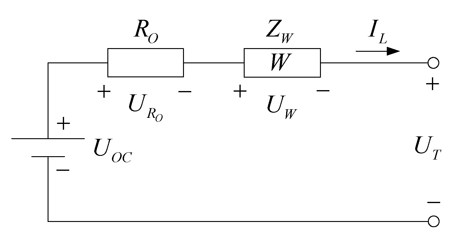
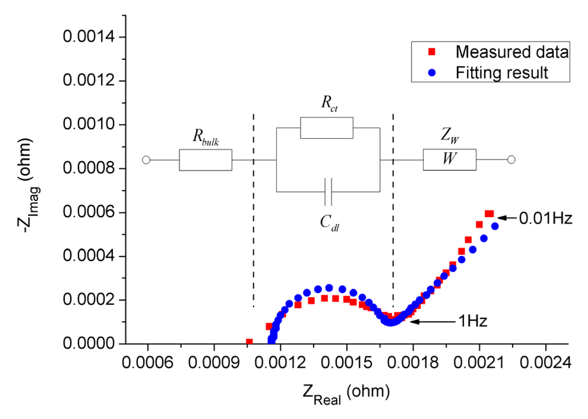
2.1.2. Simplified EIS Model

The EIS test result of a lithium iron phosphate (LiFePO₄/graphite) battery and its fitting result based on the simple EIS model are presented in Figure 2.

Figure 2. EIS test result and fitting result of the simple EIS model.

Figure 2. EIS test result and fitting result of the simple EIS model.

The values of R_ct and C_dl are 0.46 mΩ and 28.59 F, and the time constant τ is 0.01315 s. The time constant of R_ct and C_dl is very small and barely manifested on the terminal voltage in the case of electric vehicle applications. Hence, the simple EIS model can be further simplified for a LiFePO₄/graphite battery.

The impact of double layer capacitance on battery’s external characteristics can be ignored. Moreover, R_ct is assumed to be constant with current at the room temperature. Thereby, the simplified EIS model shown in Figure 3 is obtained.

Figure 3. The simplified EIS model.

Figure 3. The simplified EIS model.

The model consists of three elements: voltage source U_OC, ohmic resistance R_O and Warburg impedance Z_W. U_T and I_L denote the terminal voltage and the total current flowing through the battery, respectively.

Voltage source is used to describe the open-circuit voltage characteristics of the battery. Due to the simplification of the battery model, many chemical reaction kinetics processes and the chemical reaction boundary conditions are ignored. U_OC represents the value of the open circuit voltage (OCV), and can be expressed by Equation (1) [26]:

$$U_{OC}=E_{OC,p}\left(So{C}_p\right)-E_{OC,n}\left(So{C}_n\right)$$

(1)

where E_OC,p and E_OC,n are open circuit potentials of positive and negative electrodes. They are functions of the SoC which is determined by the average concentration of ions of each electrode. U_OC is mainly decided by three parameters: the SoC’s start points of positive and negative electrodes and the cycle range of SoC.

R_O is a pure resistance element, which mainly reflects the medium-high frequency (typically <1 Hz) impedance characteristic of EIS; the value of this parameter is approximate the sum of the battery bulk resistance R_bulk, SEI film resistance R_set and electric charge transfer resistance R_ct [27], as is shown in Equation (2):

$$\{\begin{array}{l}{R}_O=R_{bulk}+R_{sei}+R_{ct}\\ R_{bulk}=R_{ext}+R_{O,\mathrm{electrolyte}}^{eff}+R_{O,solid}^{eff}\\ R_{sei}=A\frac{{\eta }_{sei}}{I_L}\\ R_{ct}=\frac{{\eta }_{ct}}{I_L},I_L=A\cdot i_0\cdot \left(\exp \left(\frac{{\alpha }_{a}F}{RT}\right){\eta }_{ct}-\exp \left(\frac{{\alpha }_{c}F}{RT}\right){\eta }_{ct}\right)\end{array}$$

(2)

where R_ext is the connecting resistance, $R_{O,\mathrm{electrolyte}}^{eff}$ and $R_{O,solid}^{eff}$ stand for the effective part of the electrolyte ohm impedance and solid ohm impedance affecting on the terminal voltage. R_sei is mainly determined by the SEI film produced on the surface of negative electrode particles. R_ct is decided by Butler-Volmer kinetics.

Z_W is the Warburg impedance, which is usually used to describe the diffusion characteristics. It is a 0.5 order fractional element. U_W is the terminal voltage of this element. Fleischer et al. [28] presented the physical meaning of the parameters in Z_W; without considering the boundary conditions, Z_W can be expressed by Equation (3):

$$Z_W=\frac{\text{R}T}{c{n}^2{F}^{2}A}\cdot \frac{1}{\sqrt{jwD}}$$

(3)

where, R is the gas constant, T is the temperature, c represents the molar concentration of active particles, F is Faraday’s constant, A is the active surface area, D is the diffusion coefficient of the materials. Let $X_W=\frac{RT}{c{n}^2{F}^{2}A{D}^{0.5}}$, then Equation (4) can be obtained:

$$Z_W=\frac{X_W}{{\left(jw\right)}^{0.5}}$$

(4)

The characteristics of the battery from different aspects are described by the three model parameters. Meanwhile, in the simplified EIS model, charge capacity (Q) is also a crucial parameter for the batteries, and it is meaningful to battery grouping. Four battery performance parameters, Q, U_OC, R_O, X_W are used for battery grouping.

2.2. Model Parameter Identification

The simplified EIS model parameter online identification method for EVs is proposed in the authors’ previous work [29]. In the method, a model discrete state equation should be established first, and then, model parameters are identified based on the fractional joint Kalman filter algorithm. The details of the two parts are described as follows.

2.2.1. Model State Equation Establishment

The simplified EIS model has been established in Section 2.1. In this section, the state and observation equations are constructed as follows, taking the discharge current value I_L,dis as the positive value and data sampling period T_s is one second. In Equation (5), Δ^r is used as a differential operator:

$${\mathrm{\Delta }}^r=\frac{d^r}{d{t}^r}\text{, }r>0$$

(5)

where, r is the differential order. When r = 1, Δ¹ represents a one order differential operator. As the commonly used capacitor element, if its capacitance is C, the relationship of terminal voltage U_C and the current I_C flowing through this element can be expressed by Equation (6):

$${\mathrm{\Delta }}^1{U}_C=\frac{1}{C}{I}_C$$

(6)

When r is a fractional value, Δ^r represents a fractional differential operator. Similar to the capacitor, the relationship of terminal voltage U_W and the current I_L flowing through the element can be expressed as follows:

$${\mathrm{\Delta }}^{0.5}{U}_W=X_W{I}_L$$

(7)

The battery model parameters X_W, U_OC, R_O change slightly with SoC. Then, the differential equations of state and parameters can be written in the following matrix form:

$${\mathrm{\Delta }}^{\left[\begin{array}{c}0.5\\ 1\\ 1\\ 1\end{array}\right]}\left[\begin{array}{c}{U}_W\\ \begin{array}{l}{X}_W\\ U_{OC}\\ R_O\end{array}\end{array}\right]=\left[\begin{array}{cccc}0& I_L& 0& 0\\ 0& 0& 0& 0\\ 0& 0& 0& 0\\ 0& 0& 0& 0\end{array}\right]\left[\begin{array}{c}{U}_W\\ X_W\\ U_{OC}\\ R_O\end{array}\right]$$

(8)

U_T is treated as the measurement observation parameter. The observation equation is written as below:

$$U_T=U_{OC}-I_L{R}_O-U_W$$

(9)

Equation (8) can be discretized using a bilinear transformation method. Additionally, the system state noise ω and observation noise υ are considered in these equations, where these noises are assumed independent with each other. The discrete form of the state and observation equations is expressed by Equation (10):

$$\{\begin{array}{l}{\mathrm{\Delta }}^{\left[\begin{array}{c}0.5\\ 1\\ 1\\ 1\end{array}\right]}{\left[\begin{array}{c}{U}_W\\ X_W\\ U_{OC}\\ R_O\end{array}\right]}_k=\left[\begin{array}{cccc}0& \frac{I_{L,k}+I_{L,k-1}}{2}& 0& 0\\ 0& 0& 0& 0\\ 0& 0& 0& 0\\ 0& 0& 0& 0\end{array}\right]{\left[\begin{array}{c}{U}_W\\ X_W\\ U_{OC}\\ R_O\end{array}\right]}_{k-1}+\text{ω}\\ U_{t,k}=\left[\begin{array}{cccc}-1& 0& 1& -I_{L,k}\end{array}\right]{\left[\begin{array}{cccc}{U}_W& X_W& U_{oc}& R_o\end{array}\right]}_k^T+\upsilon \end{array}$$

(10)

Based on the definition of the Grünwald-Letnikov fractional differential [21,30], the discrete differential form of a fractional state variable can be written as:

$${\mathrm{\Delta }}^r{x}_k={\displaystyle \sum _{j=0}^k{\left(-1\right)}^j\left(\begin{array}{c}r\\ j\end{array}\right)x_{k-j}}, \left(\begin{array}{c}r\\ j\end{array}\right)=\{\begin{array}{c}1\\ r\left(r-1\right)\mathrm{...}\left(r-j+1\right)/j!\end{array}\begin{array}{c}\text{ for }j=0\\ \text{ for }j>0\end{array}$$

(11)

In this paper, the following definitions are made:

$${\text{γ}}_j=\text{diag}\left[\begin{array}{cccc}\left(\begin{array}{c}0.5\\ j\end{array}\right)& \left(\begin{array}{c}1\\ j\end{array}\right)& \left(\begin{array}{c}1\\ j\end{array}\right)& \left(\begin{array}{c}1\\ j\end{array}\right)\end{array}\right]$$

(12)

$$N={\left[\begin{array}{cccc}0.5& 1& 1& 1\end{array}\right]}^T$$

(13)

where x in Equation (11) is [U_W X_W U_OC R_O]^T, then, the discrete differential form of the state and parameters of the simplified EIS model can be obtained:

$${\mathrm{\Delta }}^N{x}_k=x_k+{\displaystyle \sum _{j=1}^k{\left(-1\right)}^j{\text{γ}}_j{x}_{k-j}}$$

(14)

In Equation (14), the complexity of ${\displaystyle \sum _{j=1}^k{\left(-1\right)}^j{\text{γ}}_j{x}_{k+1-j}}$ is increased with the length of time, so this feature is not suitable for engineering applications. Additionally, the battery diffusion process does not occur infinitely, as it is constrained by the boundary conditions. Thus, k is replaced with variable length L. The value of L is chosen by applying curve fitting to the experimental data. Finally, the state and observation equations can be obtained and are shown in Equation (15):

$$\{\begin{array}{l}{x}_k=\underset{f\left(x_k,I_{L,k},I_{L,k-1}\right)}{\underbrace{\left[\begin{array}{cccc}0& \frac{I_{L,k}+I_{L,k-1}}{2}& 0& 0\\ 0& 0& 0& 0\\ 0& 0& 0& 0\\ 0& 0& 0& 0\end{array}\right]x_{k-1}}}-{\displaystyle \sum _{j=1}^k{\left(-1\right)}^j{\text{γ}}_j{x}_{k+1-j}}+w\\ y_k=\underset{g\left(x_k,I_{L,k}\right)}{\underbrace{\left[\begin{array}{cccc}-1& 0& 1& -I_{L,k}\end{array}\right]x_k}}+v\\ \text{where, }\{\begin{array}{c}k\le 64,L=k\\ k>64,L=64\end{array}\end{array}$$

(15)

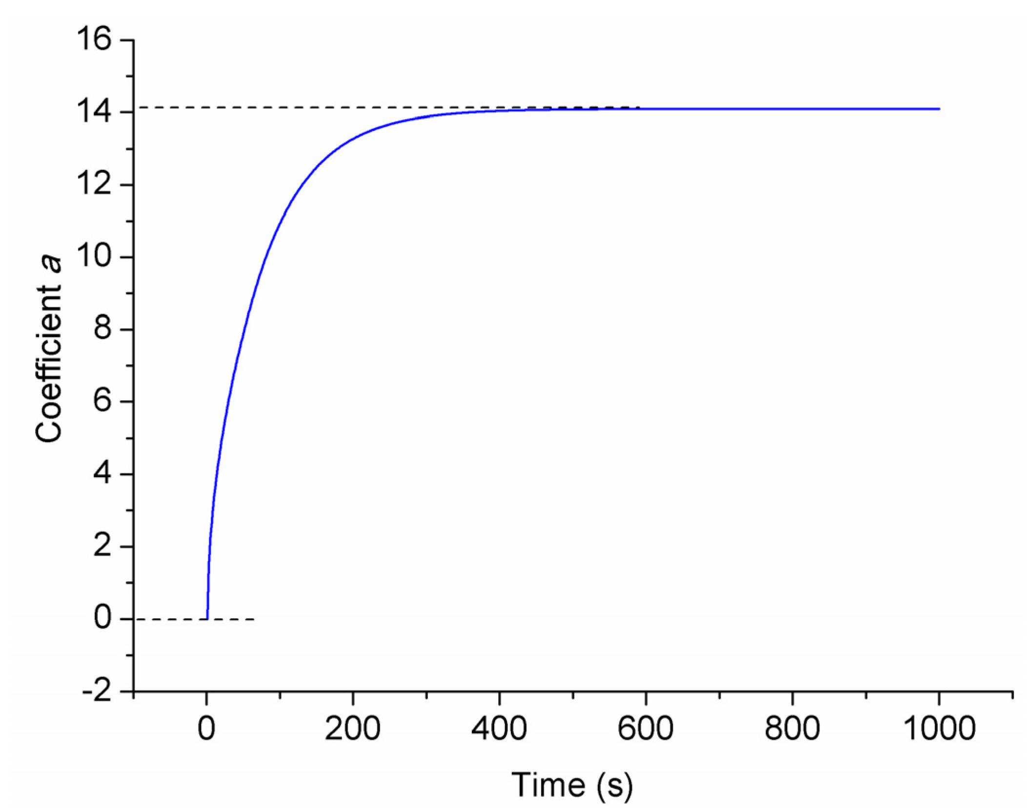
2.2.2. Model Parameter Identification

In [30], Sierociuk et al. put forward the fractional Kalman filter algorithm. In this method, fractional element state estimation, parameter identification and order estimation can be easily realized. Fractional model parameter can be estimated jointly with the state estimation. In order to distinguish the different applications, this method is called fractional joint Kalman filter (FJKF) in this paper. Based on this method, model parameter X_W is regarded as an implicit parameter of the state U_W, the value of X_W can be updated based on the state estimation result. Besides, the predication-correction feature of Kalman filter is effectively used. The application of this algorithm used in battery simplified EIS model parameter identification is described in Algorithm 1.

Algorithm 1 Model parameter identification based on FJKF.

Definitions:

$A_{k-1}={\frac{\partial f(x_{k-1},I_{L,k},I_{L,k-1})}{\partial x_{k-1}}|}_{x_{k-1}={\widehat{x}}_{k-1}^{+}}=\left[\begin{array}{cccc}0& \frac{I_{L,k}+I_{L,k-1}}{2}& 0& 0\\ 0& 0& 0& 0\\ 0& 0& 0& 0\\ 0& 0& 0& 0\end{array}\right]$

$C_k={\frac{\partial g(x_k,I_{L,k})}{\partial x_k}|}_{x_k={\widehat{x}}_k^{-}}=\left[\begin{array}{cccc}-1& 0& 1& -I_{L,k}\end{array}\right]$

Step 1: Initialization, Qk is the covariance of ωk, Rk is the covariance of noise υk. Pk is the error covariance of the state and parameter estimated values, the initial value for each parameter is give as:

${\widehat{x}}_0=E\left[x\right]$, $P_0^{+}=E\left[\left(x-{\widehat{x}}_0\right){\left(x-{\widehat{x}}_0\right)}^T\right]$

$R_0=E\left[v_0{v}_0^T\right]$, $Q_0=E\left[w_0{w}_0^T\right]$

Step 2: Time update:

State and parameter time update: ${\widehat{x}}_k^{-}=f\left({\widehat{x}}_{k-1}^{+},I_{L,k},I_{L,k-1}\right)$

Error covariance time update: $P_k^{-}=\left(A_{k-1}+{\gamma }_1\right)P_{k-1}^{+}{\left(A_{k-1}+{\gamma }_1\right)}^T+Q_x+{\displaystyle \sum _{j=2}^L{\gamma }_j{P}_{k-j}^{+}{\gamma }_j^T}$

Step 3: Measurement update:

Kalman gain matrix update: $L_k=P_k^{-}{\left(C_k\right)}^T{\left[C_k{P}_k^{-}{\left(C_k\right)}^T+R_k\right]}^{-1}$

State and parameter measurement update: ${\widehat{x}}_k^{+}={\widehat{x}}_k^{-}+L_k^x\left[y_k-g\left({\widehat{x}}_k^{-},I_{L,k}\right)\right]$

Error covariance measurement update: $P_k^{+}=\left(I-L_k{C}_k\right)P_k^{-}$

Step 4: k = k + 1, repeat Step 2 and Step 3, until all data is processed.

2.3. Parameter Identification Experiment Sequence

The battery model and model parameter identification method are described in Section 2.1 and Section 2.2. In order to obtain the battery model parameters and charge capacity, an experimental sequence is designed. The sequence is set up mainly based on dynamic stress tests, and there are seven steps.

The time consumption of this experiment is about eight hours, which is a little longer than the time consumption of constant current/voltage charge and discharge recommended by battery manufacturers, but shorter than the hybrid pulse power test described in the FreedomCAR battery test manual [31]. This sequence is described in Algorithm 2 and Figure 4.

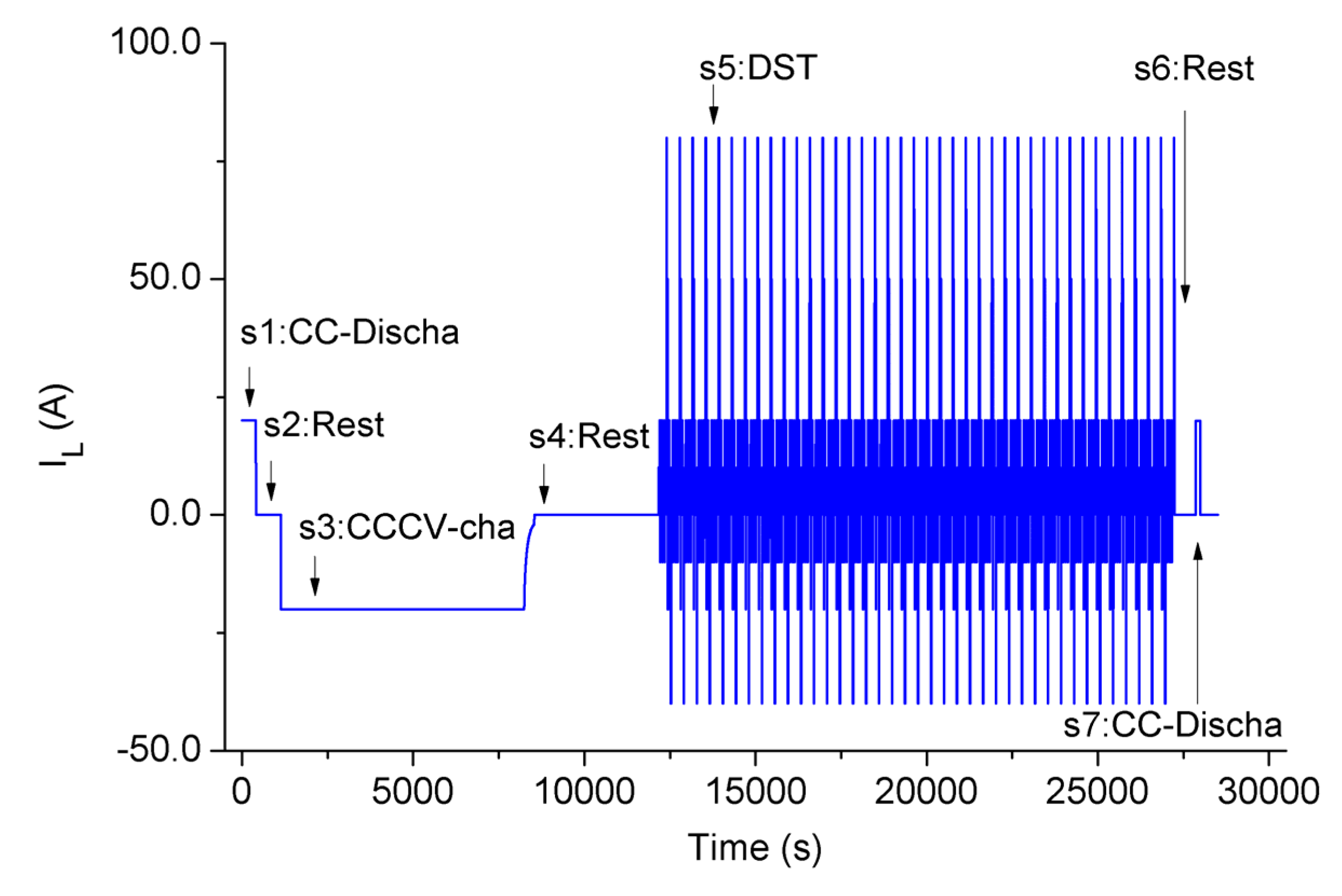
Algorithm 2 Experimental sequence for battery parameter identification.

Step 1: Constant current discharge, until battery terminal voltage reaches the lower cut-off voltage.

Step 2: Rest for one hour.

Step 3: Charge with the battery manufacturer’s recommended procedures.

Step 4: Rest for one hour.

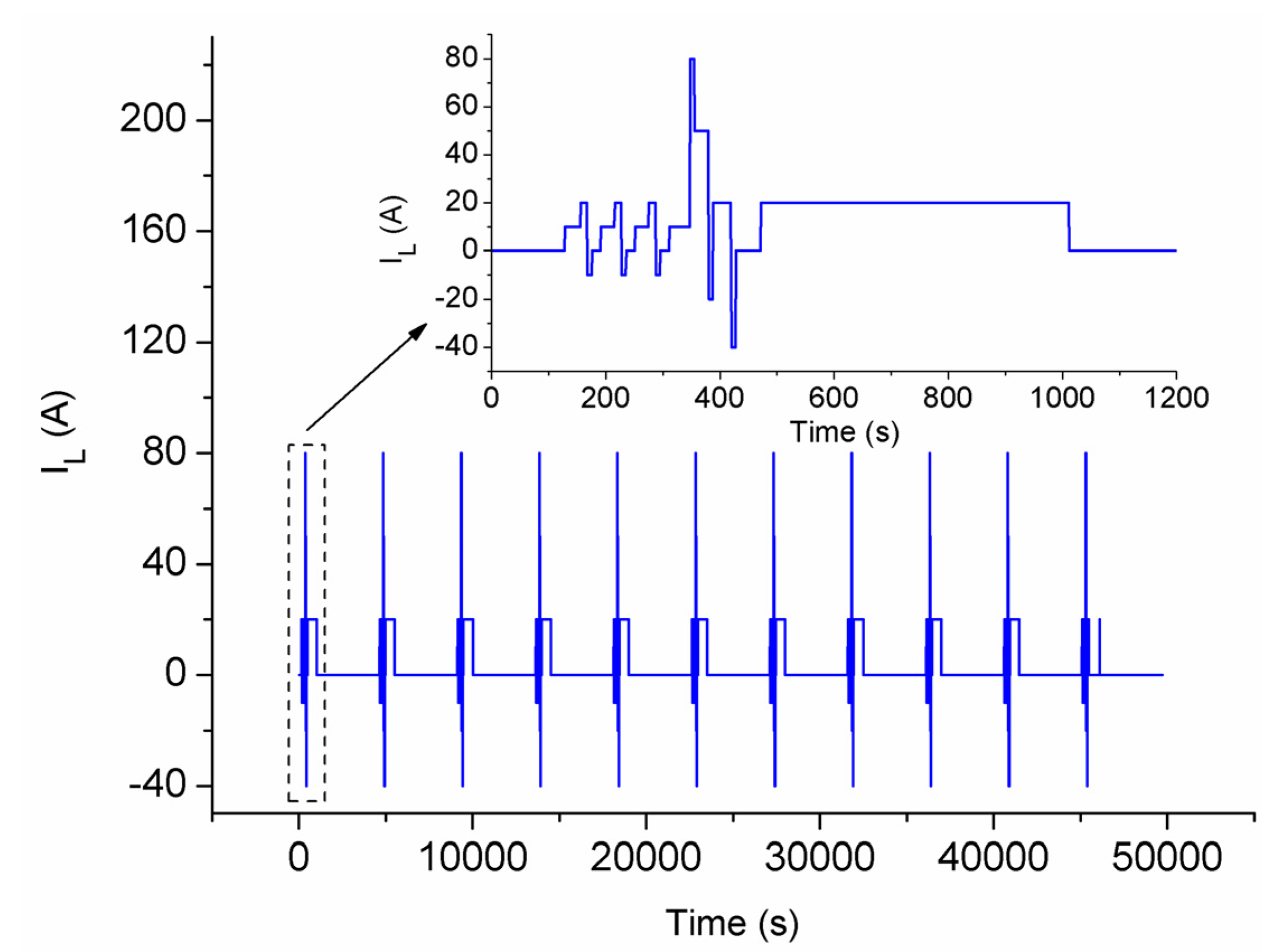
Step 5: Apply Dynamic Stress Test on the battery. The maximum discharge current is 2C in this paper. Stop when the battery terminal voltage reaches the lower cut-off voltage. The details of DST are described in FreedomCAR battery test manual.

Step 6: Rest for several minutes.

Step 7: Discharge with a low constant current, until the battery terminal voltage reaches the lower cut-off voltage. This step causes the battery to be fully discharged, this is essential for battery grouping.

Figure 4. Battery parameter identification experimental sequence.

Figure 4. Battery parameter identification experimental sequence.

3. Battery Feature Clustering

3.1. Data Preprocess

3.1.1. Data Down-Sampling

Battery model parameters U_OC, R_O, X_W can be obtained based on the method proposed in Section 2, and they are functions of test time. It is necessary to translate the function into the depth of discharge (DoD) of the battery. DoD of a battery i at time k is defined by Equation (16):

$$Do{D}_i\left(k\right)=\frac{{\displaystyle {\int }_{t=0}^{t=k}{I}_{L}dt}}{Q_i}\times 100\%$$

(16)

Here, Q_i is the charge capacity of battery i , its value can be calculated by the Ah-counting method, and this process is expressed by Equation (17):

$$Q_i={\displaystyle {\int }_{step5}^{step7}{I}_{L}dt}$$

(17)

In order to reduce the amount of calculations, a down-sampling process is executed on the parameter identification results. Additionally, model parameter identification results of DoD = 0%–10% and 90%–100% are discarded from further analysis.

3.1.2. Crude Data Exclusion

Typically, operational errors are unavoidable in the experimental process. For example, test cables may connect unreliably, equipment channels fail and so on. Apart from these errors, the failures in the battery production process can also lead to the existance of crude values in the model parameter identification results. In this paper, the crude values are discarded based on the Laiyite criterion (3σ criterion). Additionally, since the number of samples remaining should not larger than the designed numbers n₀ for battery grouping, another step is added to the crude data discarding process. The details of this process are shown in Algorithm 3.

Algorithm 3 Crude data excluding process.

Step 1: Calculate the average curve of each model parameters of the samples, additionally, calculate the average value of battery capacities.

$X_{avg}\left(DoD\right)=\frac{1}{n}{\displaystyle \sum _{i=1}^{n}X\left(DoD\right)}$

Where, X represents UOC, RO or XW.

Step 2: Calculate the average distance between the parameter curve and the average curve, that is the distance between battery capacities and the average capacity.

$D_{X,i}=mean\left(X_i\left(DoD\right)-X_{avg}\left(DoD\right)\right),i=1,\mathrm{...},n$

Step 3: Calculate the standard deviation of each distance parameter.

${\sigma }_X=\sqrt{\frac{1}{n}{\displaystyle \sum _{i=1}^n{D}_{X,i^2}}}$

Step 4: Discard the samples that do not meet the requirement of Laiyite criterion. The Laiyite criterion is: $\left|D{X}_i\right|<3{\sigma }_X$

Step 5: Regard the remaining samples as the evolution objects. Reset the number of evolution objects n, and repeat Steps 1–4, until all the remaining parameters are eligible with the requirement of Laiyite criterion.

Step 6: If $n>n_0$, randomly discard the samples which have maximum value of $\left|D{X}_i\right|$ until the number of remaining samples is equal to $n_0$. Ultimately, the samples used for battery grouping are obtained.

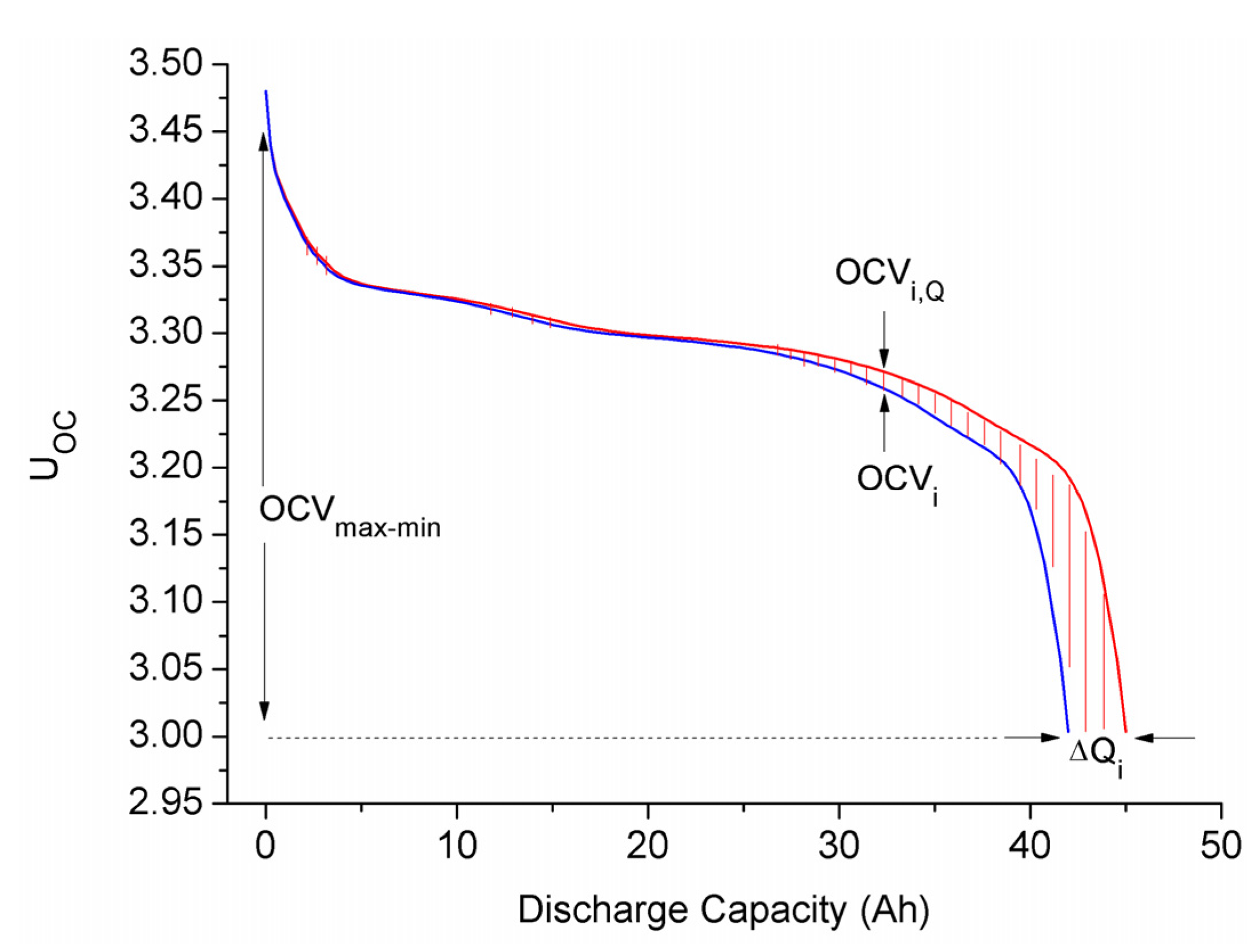
3.2. Consistency Evaluation Parameter Generation

In Section 3.1, $D_Q$, $D_{U_{OC}}$, $D_{R_O}$ and $D_{X_W}$ of each remaining battery are obtaine; these parameters have different units and should be normalized for further analysis, the results are represented by $D_Q^{*}$, $D_{U_{OC}}^{*}$, $D_{R_O}^{*}$ and $D_{X_W}^{*}$. The four parameters describe the performance of batteries, but cannot be used directly for battery consistency evaluation, because they have different effects on battery consistency. It is necessary to weight the parameters according to defined rules. In this paper, the weights are set up based on the parameters’ inconsistent influence on the terminal voltage. Battery terminal voltage can be expressed as:

$$U_T=U_{OC}-U_{R_O}-U_W$$

(18)

The relationship between Q’s inconsistent value ΔQ and ΔU_OC is described in Figure 5. In order to simplify the calculation, the OCV curve can be regard as a straight line, and Equation (19) can be obtained.

Figure 5. Effect of capacity inconsistency on U_OC (U_T).

Figure 5. Effect of capacity inconsistency on U_OC (U_T).

$$\mathrm{\Delta }{U}_{T,Q}=\frac{\frac{1}{2}\mathrm{\Delta }OC{V}_{\max -\min }\mathrm{\Delta }Q}{Q_{avg}}$$

(19)

where, $\mathrm{\Delta }OC{V}_{\max -\min }$ is about 0.48 V.

The relationship between ΔU_T and ΔU_OC, ΔR_O can be easily obtained; this are expressed as:

$$\mathrm{\Delta }{U}_{T,U_{OC}}=\mathrm{\Delta }{U}_{OC}$$

(20)

$$\mathrm{\Delta }{U}_{T,R_O}=I_L\mathrm{\Delta }{R}_O$$

(21)

However, the influence of ΔX_W on ΔU_T cannot be obtained directly. Thus, the following analysis is carried out. Assuming the initial state of U_W is zero, when a step current excitation I_L is applied to Z_W, the voltage response after k s can be calculated. When k = 1, the voltage response is given as:

$$U_{W,1}=X_W{I}_L-{\left(-1\right)}^1\left(\begin{array}{c}0.5\\ 1\end{array}\right)U_{W,0}$$

(22)

The voltage response of Z_W when k ≥ 2 is given as:

$$U_{W,k+1}=X_W{I}_L-{\displaystyle \sum _{j=1}^L{\left(-1\right)}^j\left(\begin{array}{c}0.5\\ j\end{array}\right)U_{W,k+1-j}}$$

(23)

Finally, the voltage response of Z_W at time k can be given as:

$$U_{W,T}=a\left(k\right)X_W{I}_L$$

(24)

where, a(k) is coefficient variable of X_WI_L, and is determined by L in the state discrete equations. I_L and X_W are constant, the coefficient a can be expressed in Figure 6. The maximum value of a is a_max(k) = 14.

Figure 6. Changes of the coefficient a with time.

Figure 6. Changes of the coefficient a with time.

During charge or discharge, the working time is much longer than the length of time presented in the figure. a_max = 14, the value of a changes mainly near the maximum value. The relationship between ΔU_T and ΔX_W can be described as:

$$\mathrm{\Delta }{U}_W=a_{\max }{I}_L\mathrm{\Delta }{X}_W$$

(25)

The median working current 1C (40 A) is used as the reference current I_L,ref in the Equations (24) and (25), the weight proportion of each parameter can be described as:

$$w_Q:w_{U_{OC}}:w_{R_O}:w_{X_W}=\frac{\frac{1}{2}OC{V}_{\max -\min }\mathrm{\Delta }Q}{Q_0}:\mathrm{\Delta }{U}_{OC}:I_{L,ref}\mathrm{\Delta }{R}_O:a_{\max }{I}_{L,ref}\mathrm{\Delta }{X}_W$$

(26)

After the parameters are weighted, the feature vector $Cell\left(D_{Q,w}^{*},D_{U_{OC},w}^{*},D_{R_O,w}^{*},D_{X_W,w}^{*}\right)$ which consists of four consistency evaluation parameters for each cell is obtained.

3.3. Battery Equal-Number Clustering

Battery grouping is a special kind of clustering problem. In the traditional clustering method, elements are grouped based on the similarity of feature data, and there is no pre-set category features. The whole clustering process works without supervision. However, battery grouping is a little different from the traditional method, because the amount of elements in each group should meet the requirements of the battery pack. Hence, a special equal-number clustering method is needed for battery grouping.

3.3.1. K-Means Clustering Method

K-means clustering method is a popular partitioning clustering method [32]. In this method, the initial cluster centers are randomly selected from the elements to be clustered, and the remaining elements are clustered into N groups based on the similarity (distance), and the cluster center of each cluster is recalculated after that. The variance function shown in Equation (27) is generally used as the standard measurement function in this method. The main steps of K-means are shown in Algorithm 4.

$$E={\displaystyle \sum _{n=1}^N{\displaystyle \sum _{x\in c_n}{\Vert x-{\text{μ}}_n\Vert }^2}}$$

(27)

Algorithm 4 Main steps of K-means clustering method.

Step 1: Initialize the cluster centers. Select N cluster centers randomly. ${\text{μ}}_1,{\text{μ}}_2,\mathrm{...},{\text{μ}}_k$.

Step 2: Calculate the distance between each sample and each cluster center. Clustering the samples to the nearest cluster based on the minimum distance principle. For sample p, it is belong to the cluster which is obtained by: $c^{\left(p\right)}=\arg \min {\Vert x^{\left(p\right)}-{\text{μ}}_n\Vert }^2$

Step 3: Recalculate the cluster centers. The mean value of each cluster is used as the new cluster center:

${\text{μ}}_n=\frac{{\displaystyle \sum _{p=1}^{M}1\left\{c^{\left(p\right)}=n\right\}{x}^{\left(p\right)}}}{{\displaystyle \sum _{p=1}^{M}1\left\{c^{\left(p\right)}=n\right\}}}$

Step 4: Repeat Step 2 and Step 3, until the cluster centers are no longer changing or only changes minimal.

3.3.2. Kd-Tree Cluster Center Initialization

Unfortunately, K-means clustering method is local optimization strategy, and it is sensitive to the initial cluster center and can easily fall into a local optimal solution. A good initial cluster center can avoid the local optima issue. Redmond, et al. proposed a cluster center initial method based on kd-tree. kd-tree is established for data density estimation, and the initial cluster centers are selected from kd-tree’s leave boxes based on an improved max-min distance method. This cluster center initial method is much better than the random cluster center initial method. The calculation is relatively simple. Readers can refer to [33] for further details of the algorithm.

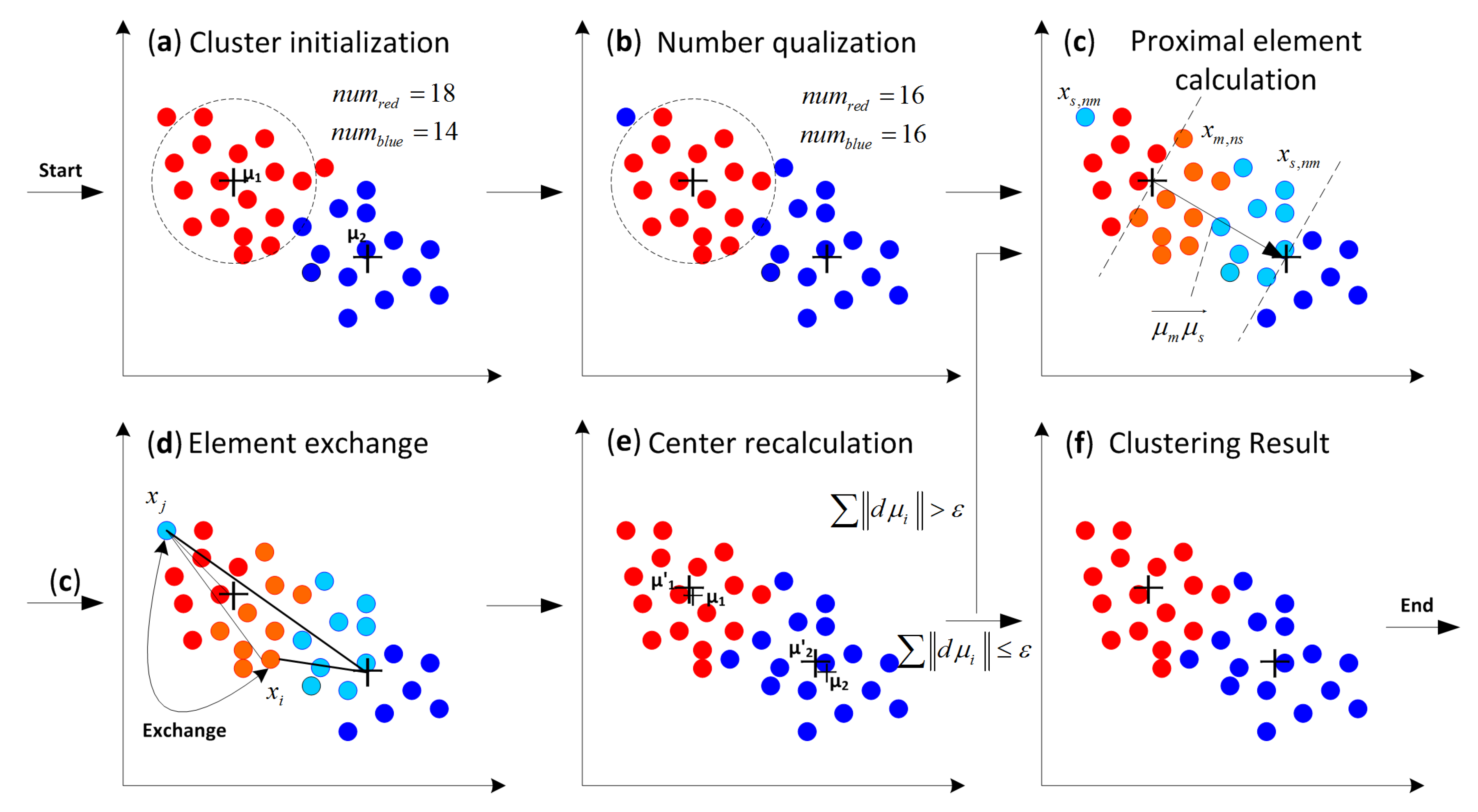
3.3.3. The New Modified K-Means Clustering Method

Section 3.3.1 and Section 3.3.2 describe the K-means clustering method using kd-tree cluster center initialization. The battery equal-number clustering method proposed in this paper is based on this method and the clustering rules are redesigned. The target of the method is partitioning the samples into N clusters and the amount of elements in each cluster is equal to M. The objective function of equal-number clustering is the same with the traditional K-means method, as shown in Equation (27). An adjusting rule is developed to equalize the numbers as below:

Rule 1: Element number equalization

The cluster which has the largest number of elements should be determined first. Then, the elements of this cluster are sorted based on the distances between them and their cluster center. The element with the farthest distance is assigned to another cluster whose number of elements is less than the pre-set value M and the distance of this element to the new cluster should be as near as possible. This assigning rule takes distance and element number into account at the same time. We repeat this process until the number of elements in each cluster is equal to the pre-set value. Equal-number clusters can be accomplished based on Rule 1. However, this process cannot guarantee the accuracy of the element’s attribution. Thus, an element exchange criterion between two clusters is set up.

Rule 2: Element exchange criterion

This rule is made to regulate the element exchanging process between two selected clusters. In order to explain this rule, several definitions are made:

Master cluster $C_m$: $C_m$ is the cluster who initiates the element exchange process. The cluster center and element $i$ in this cluster is expressed by ${\text{μ}}_m$ and $x_{m,i}$.

Slave cluster $C_s$: $C_s$ is the cluster waiting for element exchange with $C_m$. The cluster center and element j is expressed ${\text{μ}}_s$ and $x_{s,j}$.

Master (Slave) center vector $\overrightarrow{{\text{μ}}_m{\text{μ}}_s}$ ($\overrightarrow{{\text{μ}}_s{\text{μ}}_m}$): The vector’s starting point is ${\text{μ}}_m$ (${\text{μ}}_s$) and ending point is ${\text{μ}}_s$(${\text{μ}}_m$).

Master (Slave) proximal element $x_{m,ns}$ ($x_{s,nm}$): The element of $C_m$ ($C_s$) near ${\text{μ}}_s$ (${\text{μ}}_m$). If $\overrightarrow{{\text{μ}}_m{x}_{m,i}}\cdot \overrightarrow{{\text{μ}}_m{\text{μ}}_s}>0$, element $i$ is a Master proximal element Similarly, If $\overrightarrow{{\text{μ}}_s{x}_{s,j}}\cdot \overrightarrow{{\text{μ}}_s{\text{μ}}_m}>0$, element j is a slave proximal element.

In these two clusters, the exchange process is only allowed in the proximal elements because the exchange possibility between two proximal elements is much higher than between non-proximal elements. This limitation is an effective approach to reduce calculation complexity and improve the convergence rate of the clustering algorithm.

In order to decrease the value of the measurement target of the new modified K-means method, exchange process between $C_m$ and $C_s$ occurs when the requirements of Equation (28) is satisfied:

$${\Vert x_{m,i}-{\text{μ}}_m\Vert }^2+{\Vert x_{s,j}-{\text{μ}}_s\Vert }^2>{\Vert x_{s,j}-{\text{μ}}_m\Vert }^2+{\Vert x_{m,i}-{\text{μ}}_s\Vert }^2$$

(28)

Based on the analysis and two new rules for cluster elements attribution, the new modified K-means method is established. This equal-number clustering steps are described in the Algorithm 5 and some of the main steps are shown in Figure 7.

Algorithm 5 Steps of equal-number clustering method.

Step 1: Cluster centers initialization. Cluster center is calculated using the kd-tree cluster center initialization method.

Step 2: Cluster initialization. The elements are clustered to each cluster according to the minimum distance criterion described in K-means clustering method. Step1 and Step 2 are shown in Figure 7a.

Step 3: Element number equalization. Equalize the number of each cluster according to rule 1. This step is shown in Figure 7b.

Step 4: Distance data storage. Two arrays are set up for each cluster, named main storage array and auxiliary storage array. Calculate the distances from each element to all centers. The results are stored in the main storage arrays, but auxiliary storage array is not used here.

Step 5: Elements exchange among the clusters.

Step 5.1: Set one of the clusters as a master cluster Cm, another one is regard as a slave cluster Cs. Find the proximal elements in these two clusters. This step is shown in Figure 7c.

Step 5.2: Select a proximal element in Cm and a proximal element in Cs as the quasi-exchange elements, If the two elements can meet the requirements of Equation (28), take out the two elements from their pervious clusters, exchange the belonging of elements and store their feature parameters in the auxiliary storage array. If not, select another proximal element in Cs as the quasi-exchange element and repeat the calculation of Equation (28) and determine whether to exchange elements or not, until all xs,nms are traversed. This step is shown in Figure 7d.

Step 5.3: Select another proximal element in Cm as the quasi-exchange element, repeat Step 5.2, until all xm,nss are traversed.

Step 5.4: Set another cluster as a new Cs, repeat Step 5.2 and Step 5.3, until all clusters apart from the master cluster are treated as a slave cluster one time for element exchange.

Step 5.5: Set another cluster as a new Cm, repeat Step 5.2, Step 5.3 and Step 5.4, until all the clusters are treated as a master cluster one time.

Step 6: Take out the data stored in the auxiliary storage array, and push them onto the main storage array of each cluster. Step 6: Recalculate the center of each cluster. This step is shown in Figure 7e.

${\mu }_n=\frac{{\displaystyle \sum _{p=1}^{M}1\left\{c^{\left(p\right)}=n\right\}{x}^{\left(p\right)}}}{{\displaystyle \sum _{p=1}^{M}1\left\{c^{\left(p\right)}=n\right\}}}$

Step 7: Repeat Steps 4–6, until cluster centers do not change or only change a little.

${\displaystyle \sum \Vert \mathrm{\Delta }{\text{μ}}_n\Vert }<\text{ε}$

Where, ε is the threshold value of process stopping, the equal-number clusters are obtained.

Figure 7. Main steps of equal-number clustering (a) Cluster initialization; (b) Element number equalization; (c) Proximal element determination; (d) Elements exchange; (e) Cluster center recalculation; (f) Result of the clustering method.

Figure 7. Main steps of equal-number clustering (a) Cluster initialization; (b) Element number equalization; (c) Proximal element determination; (d) Elements exchange; (e) Cluster center recalculation; (f) Result of the clustering method.

4. Experimental Details

Battery parameter identification and battery grouping verification experiments were implemented at CALB Co. Ltd. (Luoyang, China). A series of battery test systems were used for battery testing. Model and parameter identification verification experiments were carried out with an Arbin BT2000 battery test system in the Harbin Institute of Technology. The devices under test are 95 energy-type LiFePO₄/graphite batteries produced by CALB. The typical capacity (Q₀) is 42 Ah, cut-off voltages are 3.65 V and 2.5 V, maximum constant discharge current is 2C. The experiments were conducted at room temperature and standard atmospheric pressure.

4.1. Parameter Identification Experimental Details

The sequence of parameter identification experiment has been described in Section 2.3, this sequence is applied to the 95 batteries. The terminal voltage and load current value are recorded in the experiment.

4.2. Verification Experimental Details

There are two verification experiments in this paper. One is a model and parameter identification validation experiment, the other is a battery grouping verification experiment.

4.2.1. Model and Parameter Identification Verification Experiments

In order to validate the accuracy of the simplified EIS model and parameter identification method, a load current sequence combining the DST profile with constant current discharge profile is established. The change of DoD in each segment is 10%, the interval of every segment is 1 h. This sequence is shown in Figure 8.

Figure 8. Model and parameter identification verification experimental sequence.

Figure 8. Model and parameter identification verification experimental sequence.

A1: The segment of the test data in DoD = 50% is selected for model accuracy verification. U_OC only changes slightly in this segment, and the value of U_OC can be regarded as constant. The simulation results of the first-order RC model and the simplified EIS model are compared. Genetic algorithm (GA) is used for model parameter identification in this process.

A2: The terminal voltage of each segment’s first point is regarded as the value of U_OC at the initial time. The value of U_OC at the end point of this segment is determined by the terminal voltage of the next segment’s first point. The change of U_OC is considered to be linear with the change of DoD in the center of this segment. GA and FJKF are used to get the impedance parameters in the model. The accuracy of FJKF is verified by comparing the parameter identification results of the two methods.

4.2.2. Battery Grouping Verification Experiments

In order to verify the accuracy of the battery grouping method, typically, batteries should be connected in parallel or series and experiments performed. In this paper, the batteries are not connected in parallel or in series because the analysis is too complex and meaningful results may not be obtained. Instead of that, five simple experiments are implemented on each battery respectively. Battery grouping accuracy is evaluated by the aggregation degree of the voltage curves in each group. The experiments include: 0.5 C-rate charge and 0.5 C-rate discharge, 1 C-rate charge and 1 C-rate discharge and dynamic stress test.

5. Results and Discussion

5.1. Battery Grouping Result Analysis

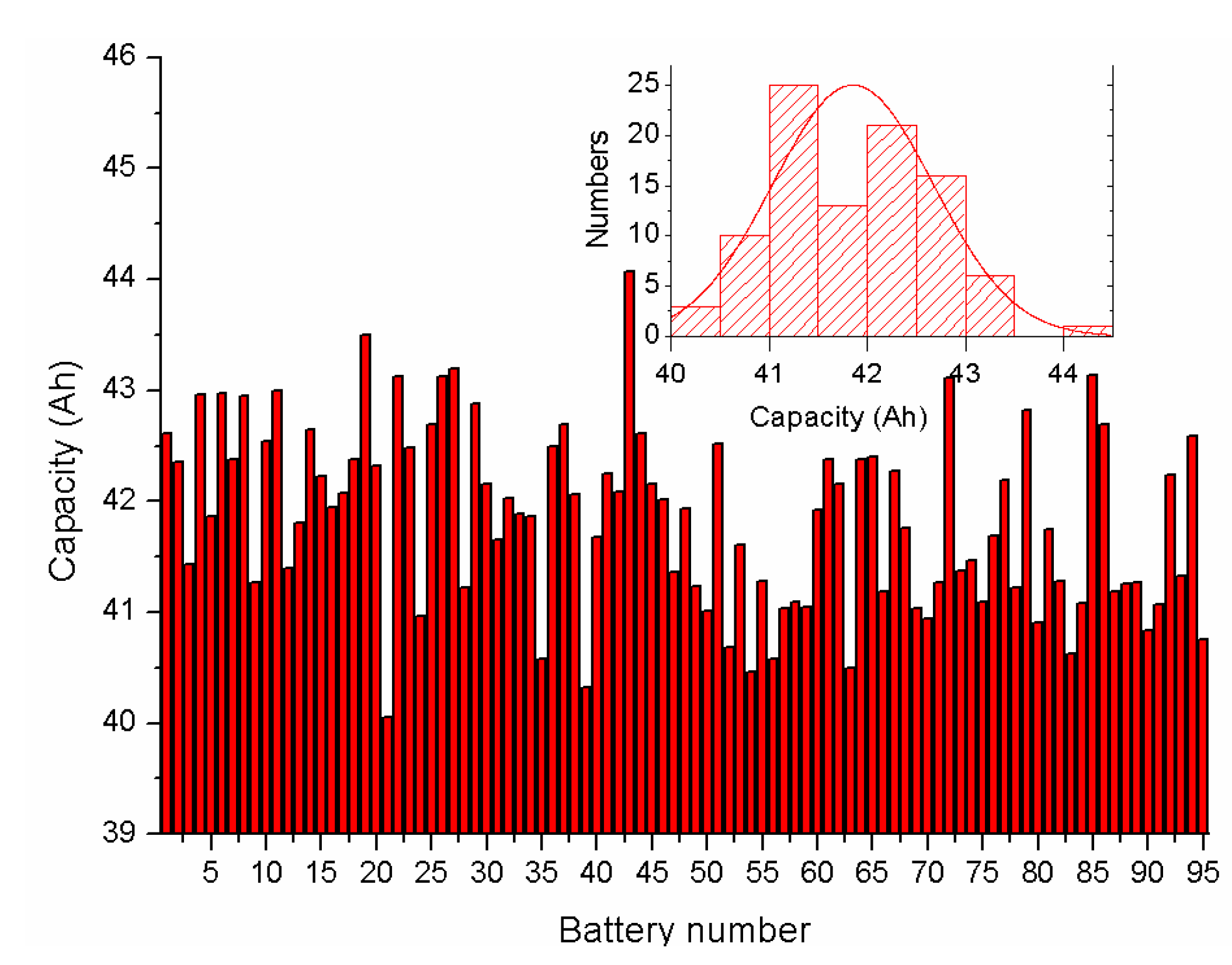
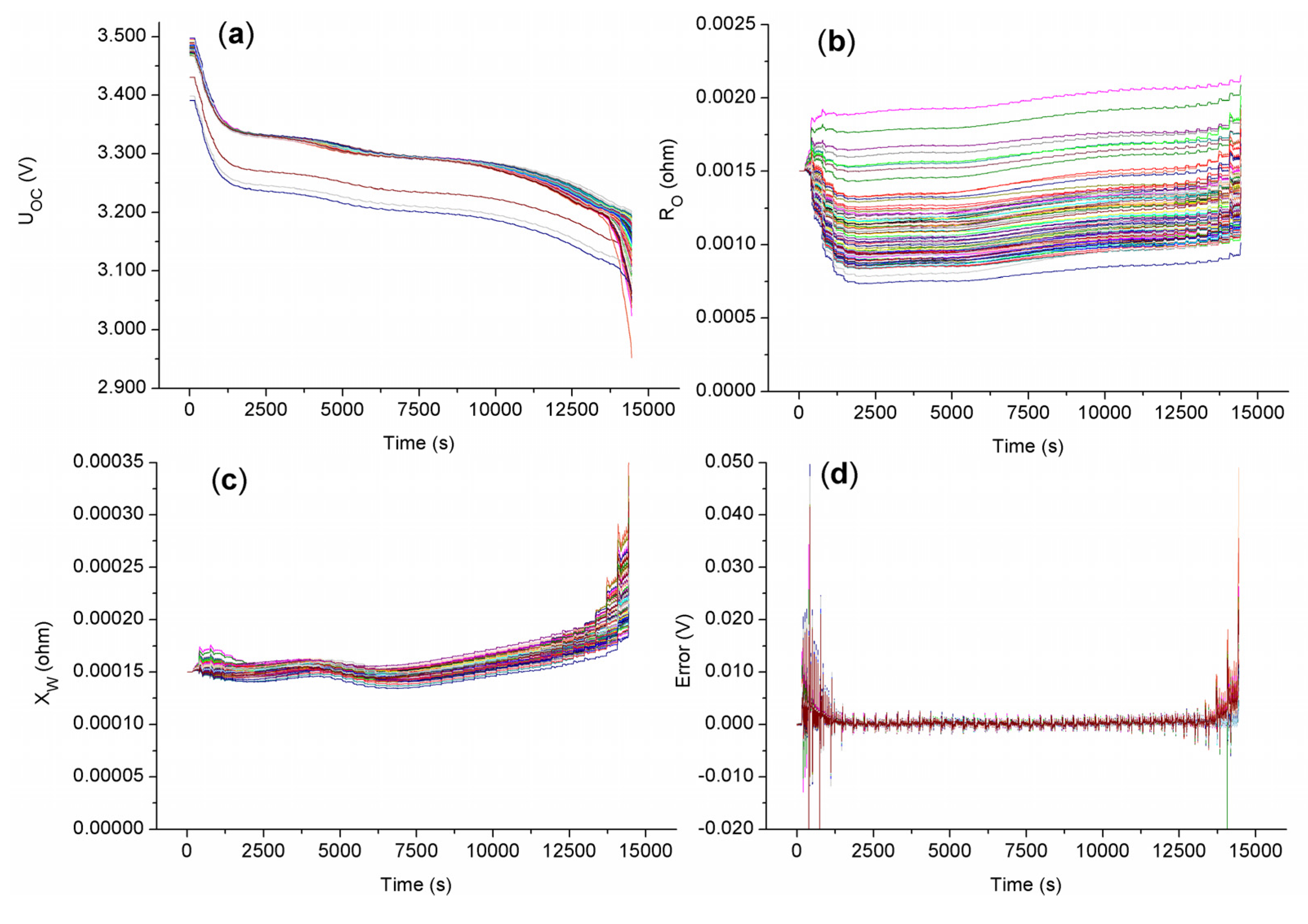
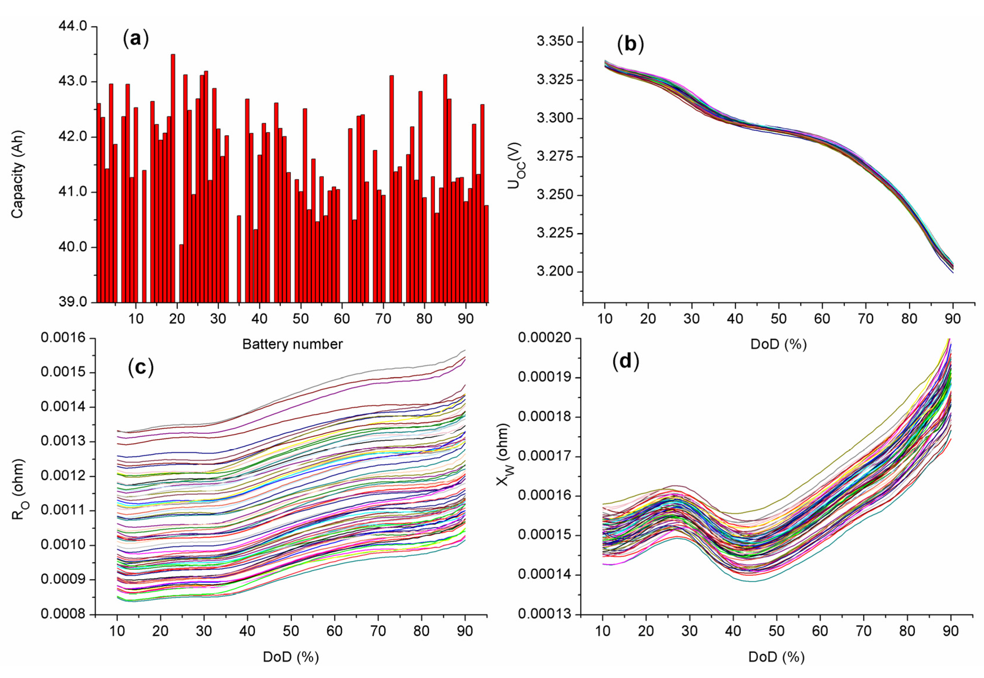
5.1.1. Battery Parameter Identification Result Analysis

Battery model parameters are extracted from the experiment using the FJKF algorithm described in Section 2.3, and battery capacity is obtained using Ah-counting. Battery capacity and its distribution are shown in Figure 9, where the capacity values are located between 40 Ah and 44 Ah, and the distribution is approximately normal. Battery model parameters and terminal voltage estimation errors are shown in Figure 10.

Figure 9. Battery capacities and distribution.

Figure 9. Battery capacities and distribution.

Figure 10. Model parameter identification result (a) U_OC; (b) R_O; (c) X_W; (d) U_T error.

Figure 10. Model parameter identification result (a) U_OC; (b) R_O; (c) X_W; (d) U_T error.

In Figure 10a,b, there exist apparent crude values in the parameter curves. In Figure 10d, the terminal voltage estimation errors in most regions (DoD = 10%–90%) are smaller than 5 mV. This phenomenon can partly verify the accuracy of the simplified EIS model and FJKF algorithm. The parameters in the regions of DoD = 0%–10% and DoD = 90%–100% is unreliable because of the large simulation error existing in these regions. The data are discarded.

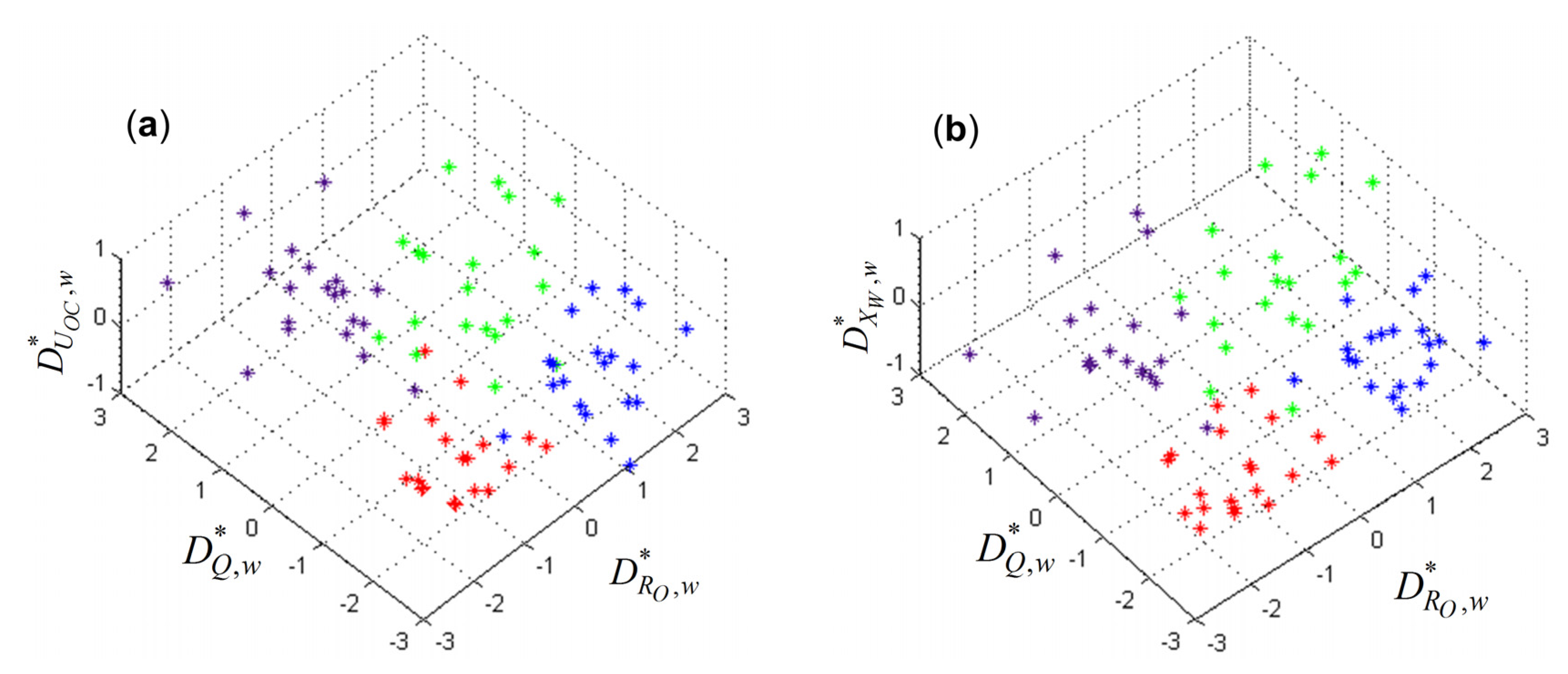
5.1.2. Battery Clustering Result Analysis

Model parameters are down sampled and the crude data is discarded according to the data preprocessing process described in Section 3.1. The result is shown in Figure 11. Then, the weights of the battery performance parameters are calculated based on Equation (26). The values of OCV_{max − min}, I_L,ref and a_max are obtained in Section 3.2 and the other coefficients in this equation can be obtained from the preprocess result shown in Figure 11:

$$\{\begin{array}{l}\mathrm{\Delta }Q=3.5\text{ Ah}\\ \mathrm{\Delta }{U}_{OC}=8.0\times {10}^{-3}\text{ V}\\ \mathrm{\Delta }{R}_O=5.0\times {10}^{-4}\text{ Ω}\\ \mathrm{\Delta }{X}_W=1.2\times {10}^{-5}\text{ Ω}\end{array}$$

(29)

Then, the weights can be obtained. After normalizing the minimum weight and rounding the value of each weight, Equation (30) can be obtained:

$$w_Q:w_{U_{OC}}:w_{R_O}:w_{X_W}\approx 3:1:3:1$$

(30)

Battery clustering result are shown in Figure 12. The samples are clustered into four groups. In each group, the consistency evolution parameters are very similar with each other.

Figure 11. The characteristic parameters after preprocess (a) Q; (b) U_OC; (c) R_O; (d) X_W.

Figure 11. The characteristic parameters after preprocess (a) Q; (b) U_OC; (c) R_O; (d) X_W.

Figure 12. Battery feature vector clustering result (a) Clustering result from the view of $D_{Q,w}^{*}$, $D_{R_O,w}^{*}$ and $D_{U_{OC},w}^{*}$; (b) Clustering result from the view of $D_{Q,w}^{*}$, $D_{R_O,w}^{*}$ and $D_{U_{OC},w}^{*}$.

Figure 12. Battery feature vector clustering result (a) Clustering result from the view of $D_{Q,w}^{*}$, $D_{R_O,w}^{*}$ and $D_{U_{OC},w}^{*}$; (b) Clustering result from the view of $D_{Q,w}^{*}$, $D_{R_O,w}^{*}$ and $D_{U_{OC},w}^{*}$.

5.2. Verification of the Battery Grouping Method

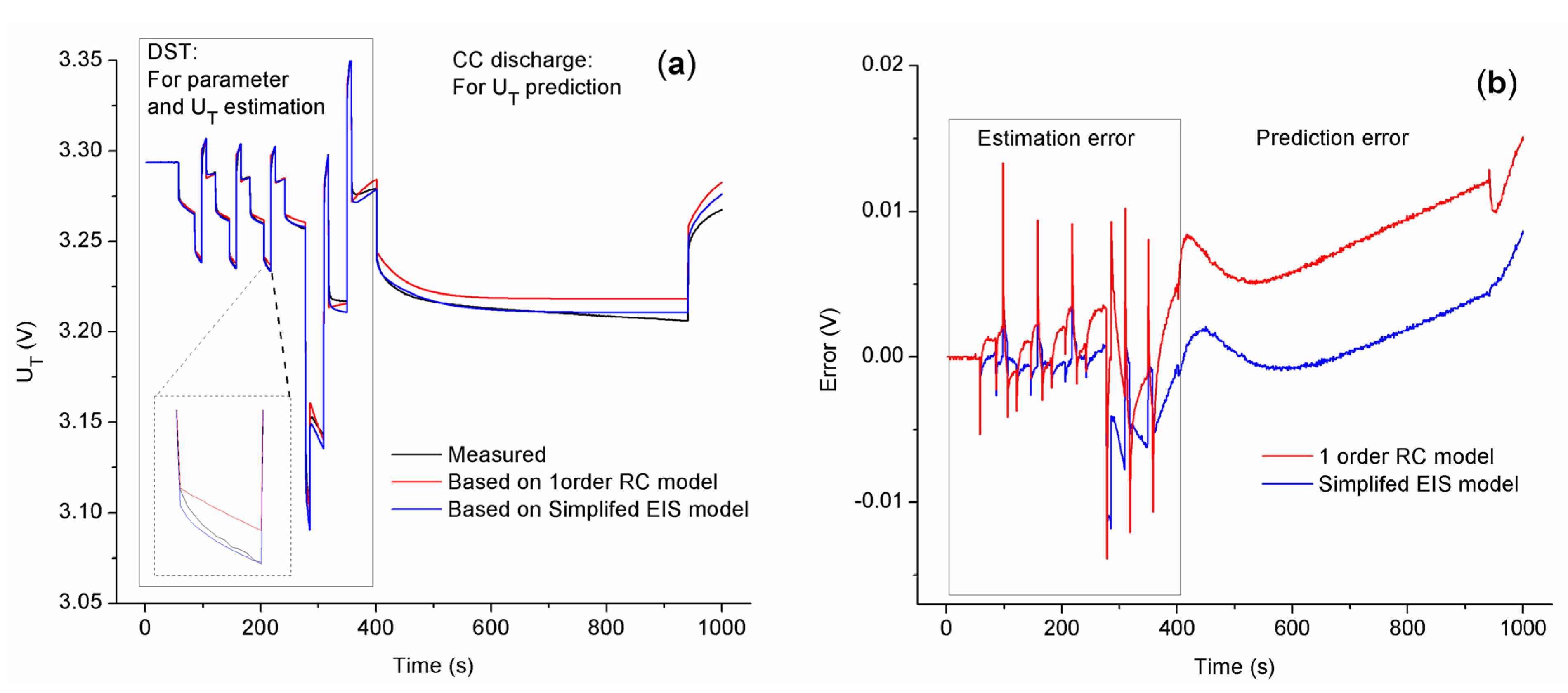
5.2.1. Model Accuracy Verification

In this section, the first order RC model is compared with the simplified EIS model. In order to obtain the model parameters, a genetic algorithm (GA) is used to find the optimal value of the parameters except for U_OC. Equation (31) is used as the objective function of GA.

$$f\left(X\right)=\frac{1}{N}{\displaystyle \sum _{k=1}^N{\left(U_{T,k}-\widehat{U_{T,k}}\right)}^2}$$

(31)

The measured terminal voltages of DST in DoD = 50% are used as the true values. The optimization results of model parameters are used for terminal voltage estimation and predication. Results are shown in Figure 13.

Figure 13. Comparison of battery model simulation results (a) simulation results and measured values of terminal voltage; (b) simulation errors.

Figure 13. Comparison of battery model simulation results (a) simulation results and measured values of terminal voltage; (b) simulation errors.

In the test results, the root mean square (RMS) voltage error of simulation results of the first-order RC model and the simplified EIS model are 6.9 mV and 2.8 mV. The estimation errors in DST region are 2.7 mV and 2.8 mV, and prediction errors are 8.7 mV and 2.7 mV. The simulation accuracy of the simplified EIS model is higher than the accuracy of the first-order RC model. Compared to the first-order RC model, the simplified EIS model can represent the impedance characteristics of the battery much better. Furthermore, the number of parameters is less than that of the first-order RC model.

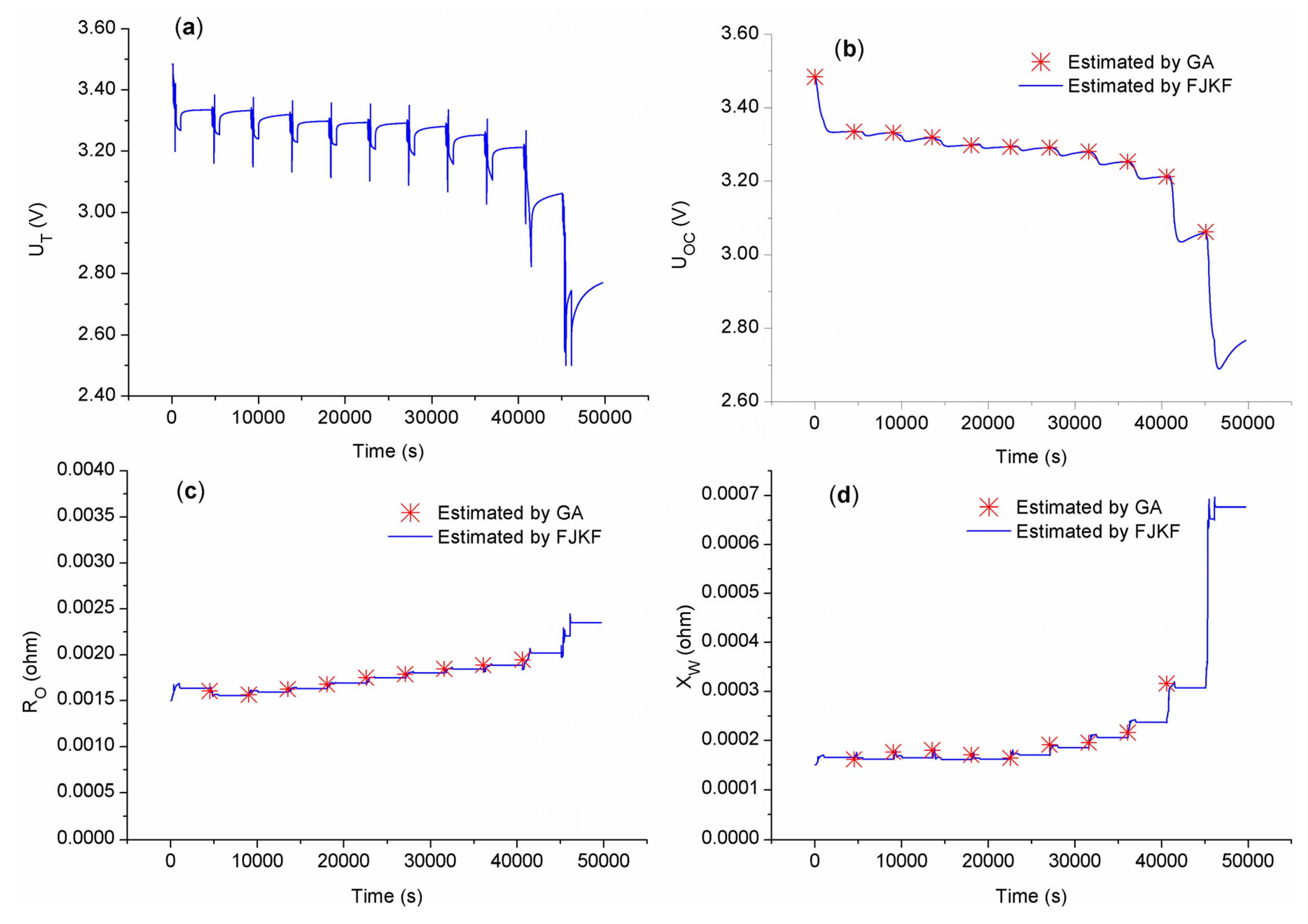
5.2.2. Model Parameter Identification Accuracy Verification

The RMS error of terminal voltage is 1.03 mV in the result which is shown in Figure 9. In this section, FJKF and GA are applied to the same experimental data for model parameter identification. The identification results of U_OC, R_O and X_W are shown in Figure 14. The results of the two methods are very similar. The accuracy and effectiveness of FJKF can be verified from the results.

Figure 14. Comparison of the model parameter identification methods: (a) terminal voltage; (b) U_OC; (c) R_O; (d) X_W.

Figure 14. Comparison of the model parameter identification methods: (a) terminal voltage; (b) U_OC; (c) R_O; (d) X_W.

5.2.3. Battery Grouping Accuracy Verification

In order to verify the validity of the proposed method for battery grouping, three other battery grouping methods—capacity matching, R_O matching and the voltage curve matching method—are used to compare with this method. The first two methods are easy to implement. The voltage curve matching method, proposed in [34], is based on the similarity of average distance, Euclidean distance and correlation coefficient, but the clustering method for three parameters was not described. In this paper, the voltage curve matching method is based on the average distance between the voltage curves and the mean curve. Additionally, 1C-rate discharge curves are used for battery grouping in this method. The clustering effective evaluation criterion is dominated based on the average Euclidean distance of the battery voltage curves of each cluster. The evaluation equation is shown as:

$$E\left({\text{group}}_i\right)=\frac{1}{N}{\displaystyle \sum _{n=1}^N\sqrt{\frac{1}{K}{\displaystyle \sum _{k=1}^K{\left(U_{T,i}\left(k\right)-U_{T,g_n}^{avg}\left(k\right)\right)}^2}}}$$

(32)

The battery grouping evaluation results of these methods are shown in Table 1. As is seen from the results, the voltage dispersion in each group after adopting the proposed clustering method is much smaller than the other ones under most working conditions, so the new grouping method has relatively higher accuracy when compared with the other methods.

Table 1. Comparison of battery grouping results.

Method	Capacity Matching (×10−3 V)			RO Matching (×10−3 V)			Curve Matching (×10−3 V)			Proposed Method (×10−3 V)
Dispersion	Max	Min	Avg.	Max	Min	Avg.	Max	Min	Avg.	Max	Min	Avg.
DST	21.56	9.483	15.40	38.43	19.18	25.94	16.50	6.910	13.41	15.80	5.682	10.78
0.5 C charge	26.02	9.406	17.00	43.61	27.31	32.71	22.78	7.803	18.22	19.60	6.425	13.98
0.5 C discharge	21.53	9.391	15.31	41.90	26.13	31.23	19.40	7.776	15.82	19.17	7.548	14.21
1 C charge	30.35	15.88	24.40	42.65	28.98	33.67	22.74	17.89	20.32	22.93	16.85	19.64
1 C discharge	24.40	16.13	20.46	42.92	27.97	32.32	23.32	9.052	17.03	21.80	9.939	16.71

Table 1. Comparison of battery grouping results.

Method	Capacity Matching (×10−3 V)			RO Matching (×10−3 V)			Curve Matching (×10−3 V)			Proposed Method (×10−3 V)
Dispersion	Max	Min	Avg.	Max	Min	Avg.	Max	Min	Avg.	Max	Min	Avg.
DST	21.56	9.483	15.40	38.43	19.18	25.94	16.50	6.910	13.41	15.80	5.682	10.78
0.5 C charge	26.02	9.406	17.00	43.61	27.31	32.71	22.78	7.803	18.22	19.60	6.425	13.98
0.5 C discharge	21.53	9.391	15.31	41.90	26.13	31.23	19.40	7.776	15.82	19.17	7.548	14.21
1 C charge	30.35	15.88	24.40	42.65	28.98	33.67	22.74	17.89	20.32	22.93	16.85	19.64
1 C discharge	24.40	16.13	20.46	42.92	27.97	32.32	23.32	9.052	17.03	21.80	9.939	16.71

6. Conclusions

A grouping method for LiFePO₄/graphite batteries is proposed. The method is mainly based on the fractional joint Kalman filter and a new modified K-means algorithm. Batteries can be divided into groups with same number of elements and similar battery characteristics in each group. The innovations and contributions of the proposed method are as follows:

• A simplified EIS battery model is adopted for battery characteristic description. The accuracy of this model is relatively higher and the number of parameters is less than in the first order RC model under the tested conditions. The model is suitable for battery grouping.
• A fractional joint Kalman filter is used for parameter identification. Fractional parameters X_W can be estimated jointly with the state U_W of the fractional element Z_W. This algorithm is appropriate and effective for fractional model parameter identification.
• A new modified K-means clustering method is proposed for battery equal-number grouping. In this method, a feature vector with four parameters is used to describe the performance of the battery from different angles. Two rules are designed to equalize the numbers of elements in each group and exchange samples among groups. The rules are added to the K-means clustering method and replace the criterion of element attribution calculation.

This battery grouping method is effective for LiFePO₄/graphite battery grouping. Furthermore, this method has the potential to be utilized in battery reuse applications. The simplified EIS model and FJKF algorithm can also be used for battery online state estimation or prediction. The equal-number clustering method can be applied to other clustering applications which require not only similarity, but also equal-numbers in each cluster. Future works will include evaluating the algorithm for the abovementioned applications.

References

1. Wang, T.; Tseng, K.J.; Zhao, J.; Wei, Z. Thermal investigation of lithium-ion battery module with different cell arrangement structures and forced air-cooling strategies. Appl. Energy 2014, 134, 229–238. [Google Scholar] [CrossRef]
2. Xiong, B.; Zhao, J.; Wei, Z.; Skyllas-Kazacos, M. Extended Kalman filter method for state of charge estimation of vanadium redox flow battery using thermal-dependent electrical model. J. Power Sources 2014, 262, 50–61. [Google Scholar] [CrossRef]
3. Wang, T.; Zhu, C.; Pei, L.; Lu, R.; Xu, B. The State of Arts and Development Trend of SOH Estimation for Lithium-Ion Batteries. In Proceedings of the 2013 IEEE Vehicle Power and Propulsion Conference (VPPC), Beijing, China, 15–18 October 2013; pp. 1–6.
4. Andre, D.; Appel, C.; Soczka-Guth, T.; Sauer, D.U. Advanced mathematical methods of SOC and SOH estimation for lithium-ion batteries. J. Power Sources 2013, 224, 20–27. [Google Scholar] [CrossRef]
5. Pei, L.; Zhu, C.; Wang, T.; Lu, R.; Chan, C.C. Online peak power prediction based on a parameter and state estimator for lithium-ion batteries in electric vehicles. Energy 2014, 66, 766–778. [Google Scholar] [CrossRef]
6. Xiong, R.; He, H.; Sun, F.; Liu, X.; Liu, Z. Model-based state of charge and peak power capability joint estimation of lithium-ion battery in plug-in hybrid electric vehicles. J. Power Sources 2013, 229, 159–169. [Google Scholar] [CrossRef]
7. Kim, J.; Shin, J.; Chun, C.; Cho, B.H. Stable Configuration of a Li-Ion Series Battery Pack Based on a Screening Process for Improved Voltage/SOC Balancing. IEEE Trans. Power Electron. 2012, 27, 411–424. [Google Scholar] [CrossRef]
8. Kim, J.; Cho, B.H. Screening process-based modeling of the multi-cell battery string in series and parallel connections for high accuracy state-of-charge estimation. Energy 2013, 57, 581–599. [Google Scholar] [CrossRef]
9. Schneider, E.L.; Oliveira, C.T.; Brito, R.M.; Malfatti, C.F. Classification of discarded NiMH and Li-Ion batteries and reuse of the cells still in operational conditions in prototypes. J. Power Sources 2014, 262, 1–9. [Google Scholar] [CrossRef]
10. Fang, K.; Chen, S.; Mu, D.; Wu, B.; Wu, F. Investigation of nickel–metal hydride battery sorting based on charging thermal behavior. J. Power Sources 2013, 224, 120–124. [Google Scholar] [CrossRef]
11. Li, X.; Wang, T.; Pei, L.; Zhu, C.; Xu, B. A comparative study of sorting methods for lithium-ion batteries. In Proceedings of the 2014 IEEE Conference and Expo Transportation Electrification Asia-Pacific (ITEC Asia-Pacific), Beijing, China, 31 August–3 September 2014; pp. 1–6.
12. Diamond, R.A.; Wang, H.; Chen, F.; Wilke-Douglas, M. Cell Preparation and Enrichment for FCM Analysis and Cell Sorting. In In Living Color; Springer Lab Manuals; Springer: Berlin/Heidelberg, Germany, 2000; pp. 111–141. [Google Scholar]
13. Guo, L.; Liu, G.W. Research of Lithium-Ion Battery Sorting Method Based on Fuzzy C-Means Algorithm. Adv. Mater. Res. 2012, 354–355, 983–988. [Google Scholar] [CrossRef]
14. Yun, W.U.; Ge-Chen, L.I.; Chen, S.L. The Application of BP Nerual Network in Battery-sorting. J. Harbin Univ. Sci. Technol. 2001, 5, 54–57. [Google Scholar]
15. Feng, F.; Lu, R.; Zhu, C. A Combined State of Charge Estimation Method for Lithium-Ion Batteries Used in a Wide Ambient Temperature Range. Energies 2014, 7, 3004–3032. [Google Scholar] [CrossRef]
16. Plett, G.L. Extended Kalman filtering for battery management systems of LiPB-based HEV battery packs Part 1. Background. J. Power Sources 2004, 134, 262–276. [Google Scholar] [CrossRef]
17. Plett, G.L. Extended Kalman filtering for battery management systems of LiPB-based HEV battery packs Part 2. Modeling and identification. J. Power Sources 2004, 134, 252–261. [Google Scholar] [CrossRef]
18. Plett, G.L. Extended Kalman filtering for battery management systems of LiPB-based HEV battery packs Part 3. State and parameter estimation. J. Power Sources 2004, 134, 277–292. [Google Scholar] [CrossRef]
19. Xiong, R.; Sun, F.; He, H.; Nguyen, T.D. A data-driven adaptive state of charge and power capability joint estimator of lithium-ion polymer battery used in electric vehicles. Energy 2013, 63, 295–308. [Google Scholar] [CrossRef]
20. Yoon, S.; Hwang, I.; Lee, C.W.; Ko, H.S.; Han, K.H. Power capability analysis in lithium ion batteries using electrochemical impedance spectroscopy. J. Electroanal. Chem. 2011, 655, 32–38. [Google Scholar] [CrossRef]
21. Xu, J.; Mi, C.C.; Cao, B.; Cao, J. A new method to estimate the state of charge of lithium-ion batteries based on the battery impedance model. J. Power Sources 2013, 233, 277–284. [Google Scholar] [CrossRef]
22. Waag, W.; Käbitz, S.; Sauer, D.U. Experimental investigation of the lithium-ion battery impedance characteristic at various conditions and aging states and its influence on the application. Appl. Energy 2013, 102, 885–897. [Google Scholar] [CrossRef]
23. Luo, W.; Lyu, C.; Wang, L.; Zhang, L. A new extension of physics-based single particle model for higher charge–discharge rates. J. Power Sources 2013, 241, 295–310. [Google Scholar] [CrossRef]
24. Fuller, T.F.; Doyle, M.; Newman, J. Relaxation phenomena in lithium-ion-insertion cells. J. Electrochem. Soc. 1994, 141, 982–990. [Google Scholar] [CrossRef]
25. Zhang, D. Modeling Lithium Intercalation of a Single Spinel Particle under Potentiodynamic Control. J. Electrochem. Soc. 1999, 147, 831–838. [Google Scholar] [CrossRef]
26. Zhang, L.; Lyu, C.; Hinds, G.; Wang, L.; Luo, W.; Zheng, J.; Ma, K. Parameter Sensitivity Analysis of Cylindrical LiFePO4 Battery Performance Using Multi-Physics Modeling. J. Electrochem. Soc. 2014, 161, A762–A776. [Google Scholar] [CrossRef]
27. Fleischer, C.; Waag, W.; Heyn, H.; Sauer, D.U. On-line adaptive battery impedance parameter and state estimation considering physical principles in reduced order equivalent circuit battery models part 2. Parameter and state estimation. J. Power Sources 2014, 262, 457–482. [Google Scholar] [CrossRef]
28. Fleischer, C.; Waag, W.; Heyn, H.; Sauer, D.U. On-line adaptive battery impedance parameter and state estimation considering physical principles in reduced order equivalent circuit battery models : Part 1. Requirements, critical review of methods and modeling. J. Power Sources 2014, 260, 276–291. [Google Scholar] [CrossRef]
29. Li, X.; Zhu, C.; Wei, G.; Lu, R. Online Parameter Estimation of LiFePO4 Battery Simplified Impedance Spectroscopy Model Based on Fractional Joint Kalman Filter. Trans. Chin. Electrotechnical Soc. 2015, in press. [Google Scholar]
30. Sierociuk, D.; DzielińSki, A. Fractional Kalman filter algorithm for the states, parameters and order of fractional system estimation. Int. J. Appl. Math. Comput. Sci. 2006, 16, 129–140. [Google Scholar]
31. FreedomCAR Battery Test Manual for Power-Assist Hybrid Electric Vehicles; U.S. Department of Energy: Washington, DC, USA, 2003.
32. Mcqueen, J. Some methods for classification and analysis of ultivariate observations. In Proceedings of the Berkeley Symposium Mathematical Statistics Probability; University of California Press: Berkeley, CA, USA, 1967; pp. 281–297. [Google Scholar]
33. Redmond, S.J.; Heneghan, C. A Method for Initialising the K-Means Clustering Algorithm Using Kd-Trees. Pattern Recognit. Lett. 2007, 28, 965–973. [Google Scholar] [CrossRef]
34. Hanze, D.Z.L.G. Cell classification system based on automatic curve-recognition. Chin. J. Power Sources 2000, 2, 65–69. [Google Scholar]