
Reinforcement Learning–Based Energy Management Strategy for a Hybrid Electric Tracked Vehicle

Abstract
:1. Introduction
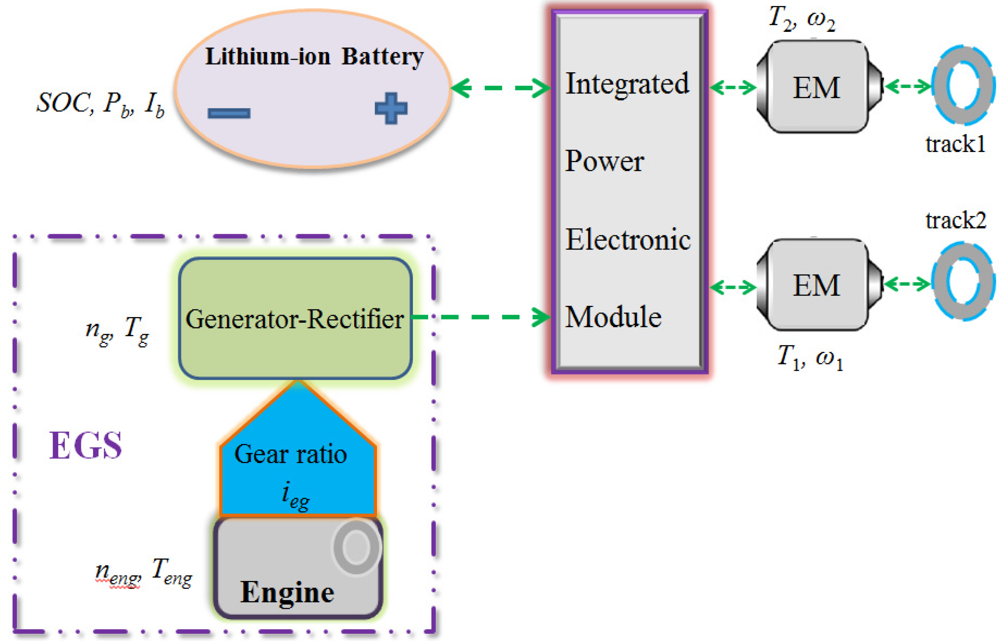
2. Hybrid Powertrain Modeling

| Parameter | Symbol | Value |
|---|---|---|
| Sprocket radius | r | 0.313 m |
| Inertial yaw moment | Iz | 55,000 kg·m2 |
| Motor shafts efficiency | η | 0.965 |
| Gear ratio param. | i0 | 13.2 |
| Vehicle tread | B | 2.55 m |
| Curb weight | mv | 15,200 kg |
| Gravit. constant | g | 9.81 m/s2 |
| Rolling resis. coefficient | f | 0.0494 |
| Contacting track width | L | 3.57 m |
| Motor efficiency | ηem | 0.9 |
| Electromotive force param. | Ke | 1.65 Vsrad−2 |
| Electromotive force param. | Kx | 0.00037 NmA−2 |
| Generator inertia | Jg | 2.0 kg·m2 |
| Engine inertia | Je | 3.2 kg·m2 |
| Gear ratio param. | ieg | 1.6 |
| Battery capacity | Qb | 50 Ah |
| Min. engine speed | neng,min | 650 rpm |
| Max. engine speed | neng,max | 2100 rpm |
| Min. SOC | SOCmin | 0.2 |
| Max. SOC | SOCmax | 0.8 |
2.1. Power Request Model
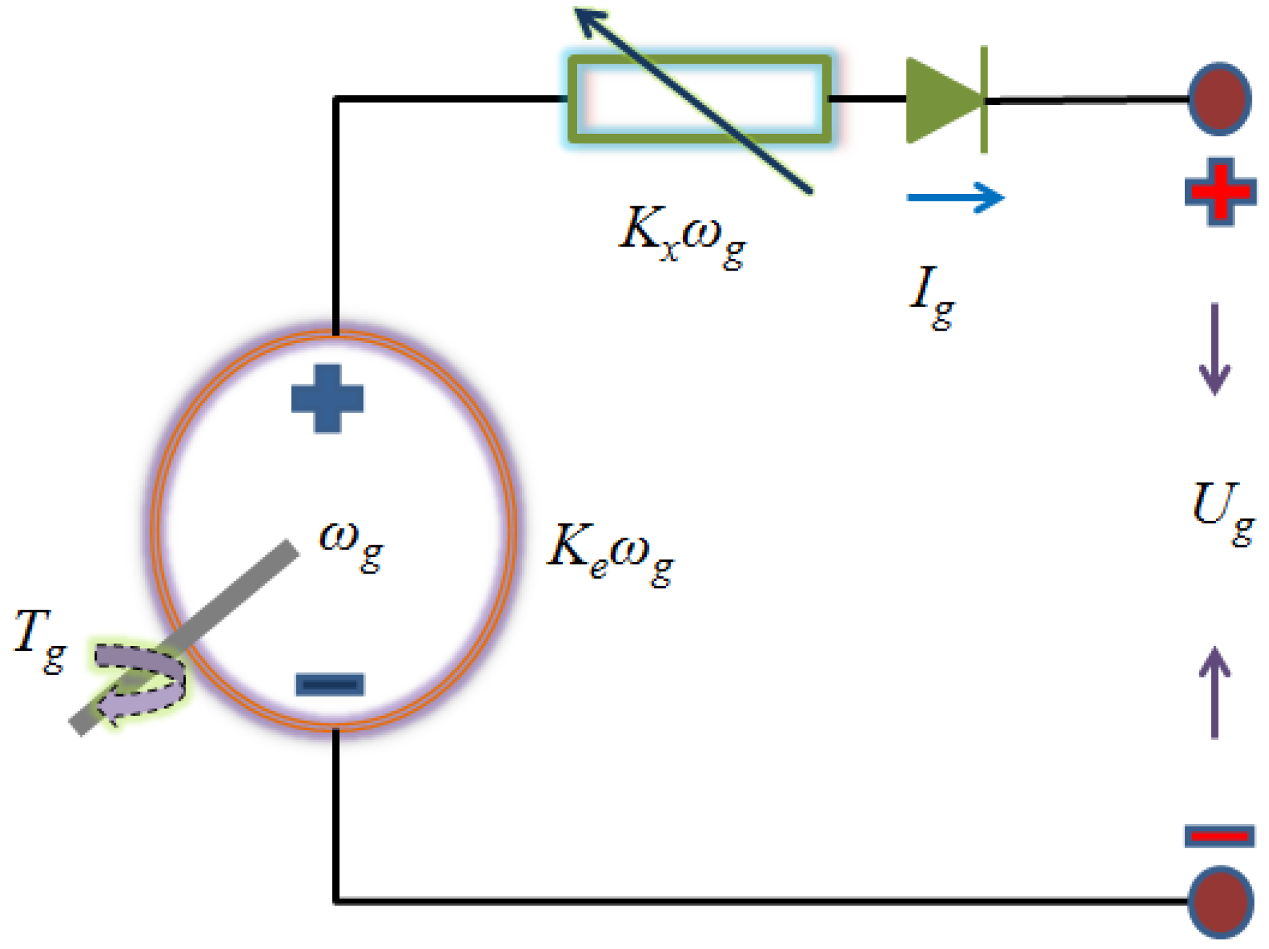
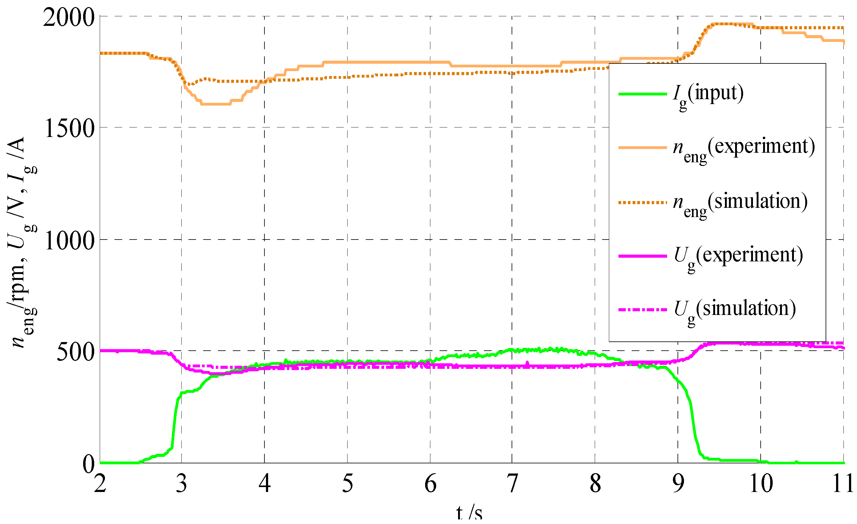
2.2. EGS Model


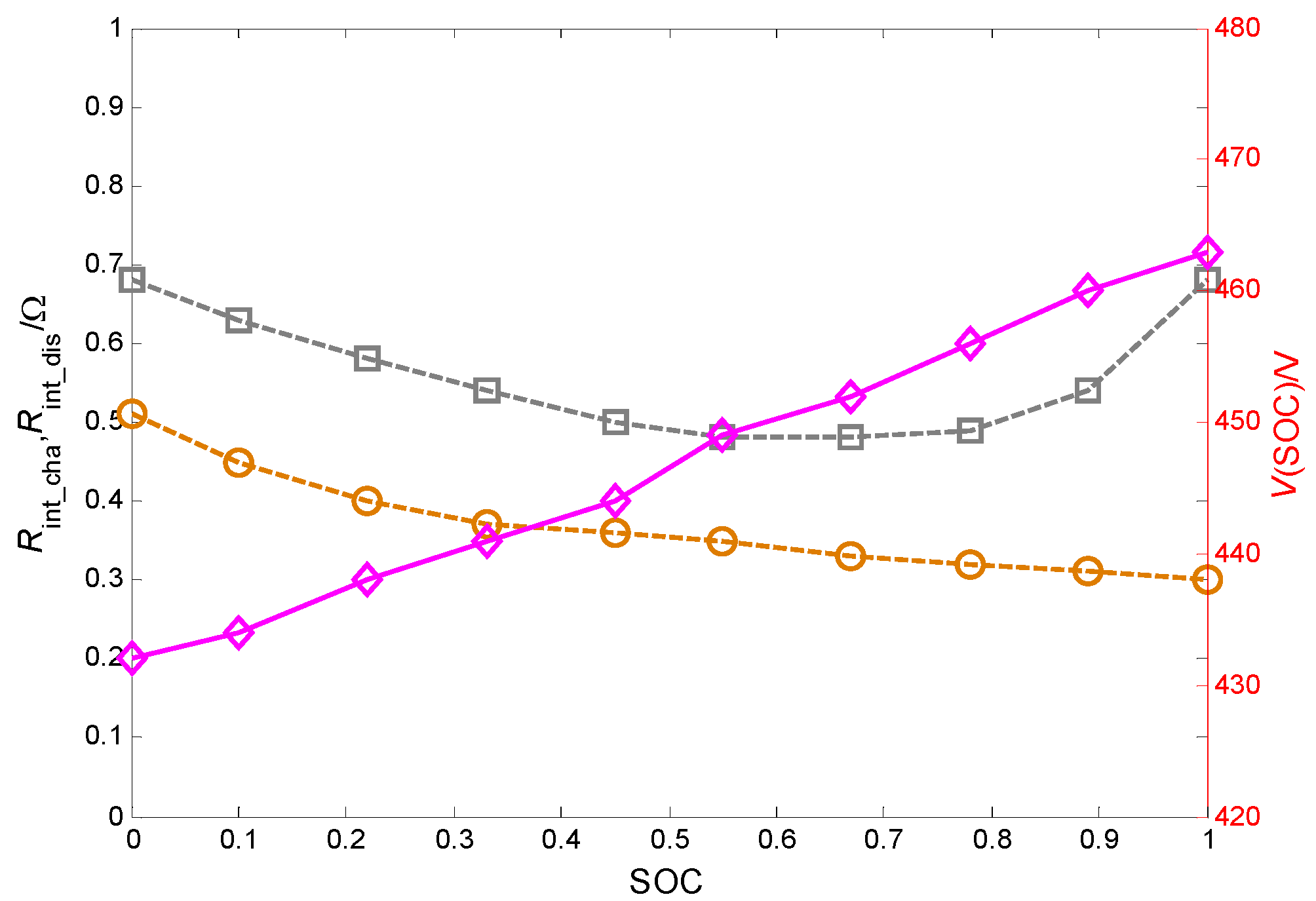
2.3. Battery Model

3. RL-Based Energy Management Strategy
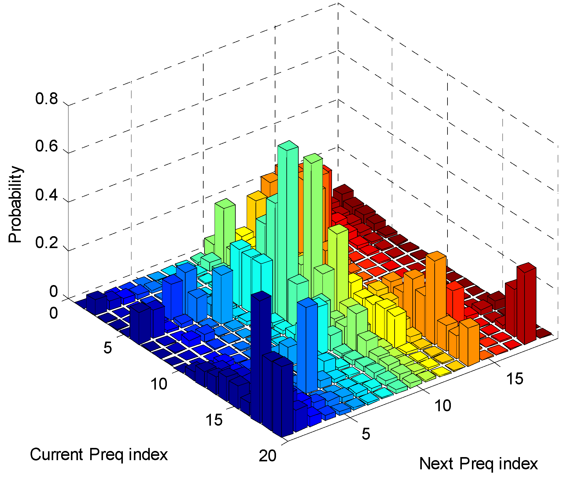
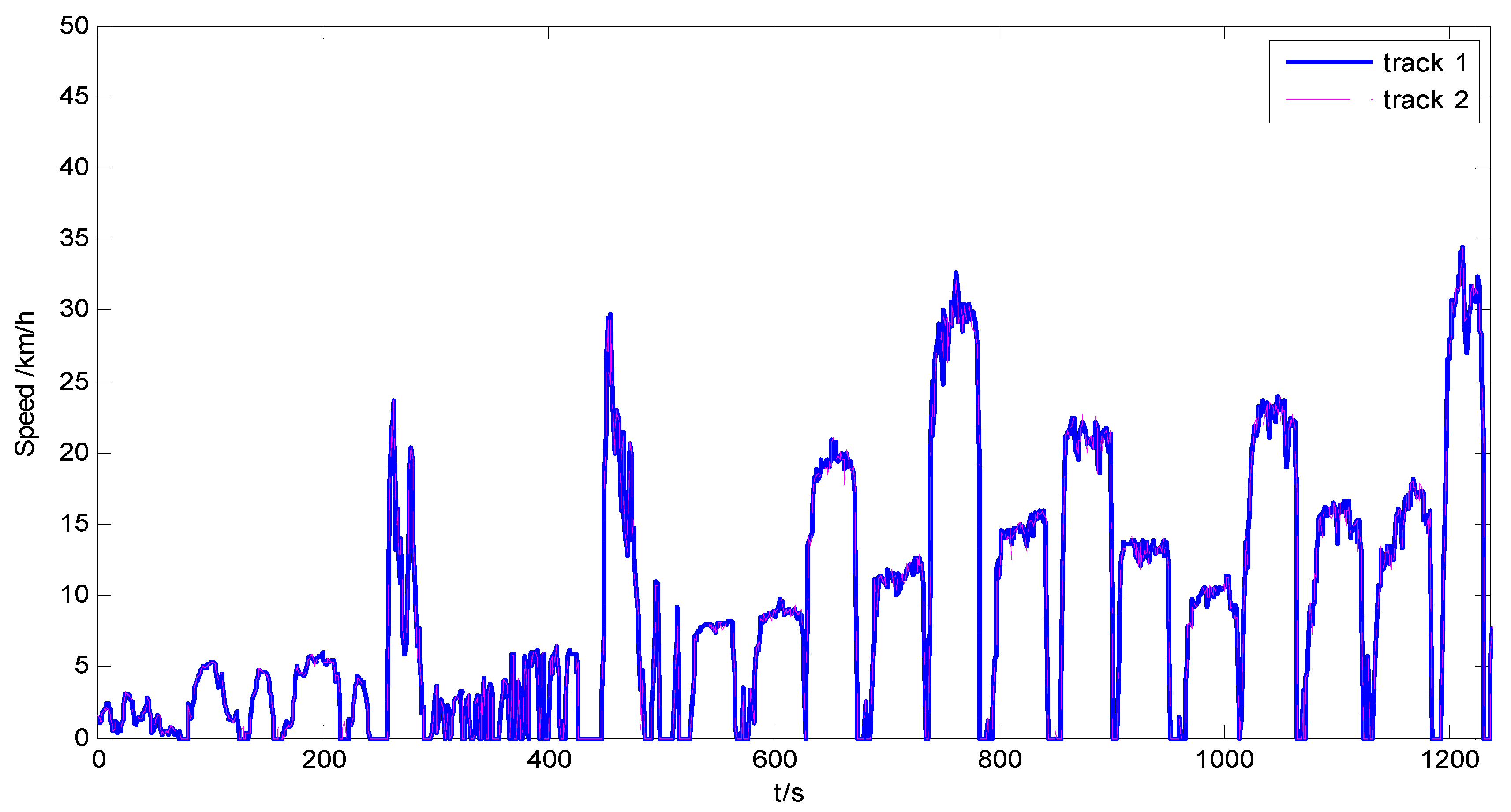
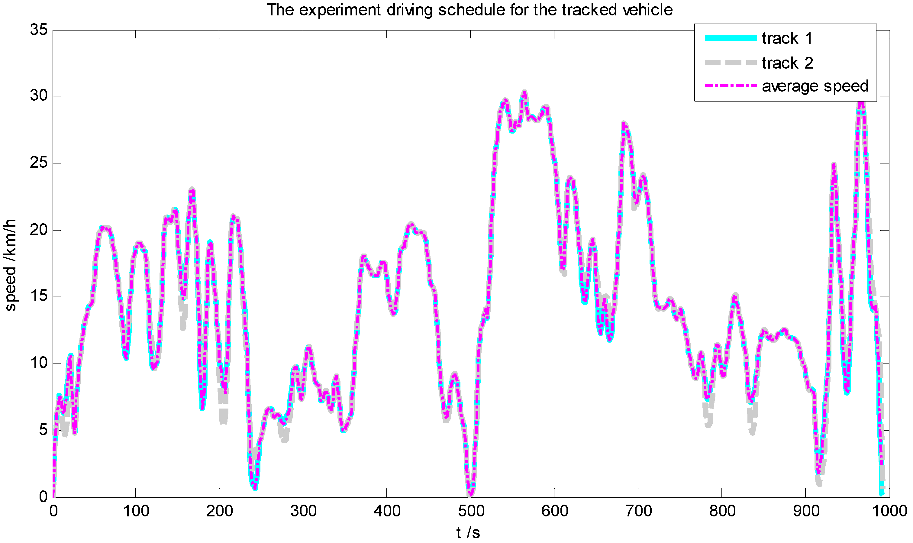
3.1. Statistic Information of the Driving Schedule


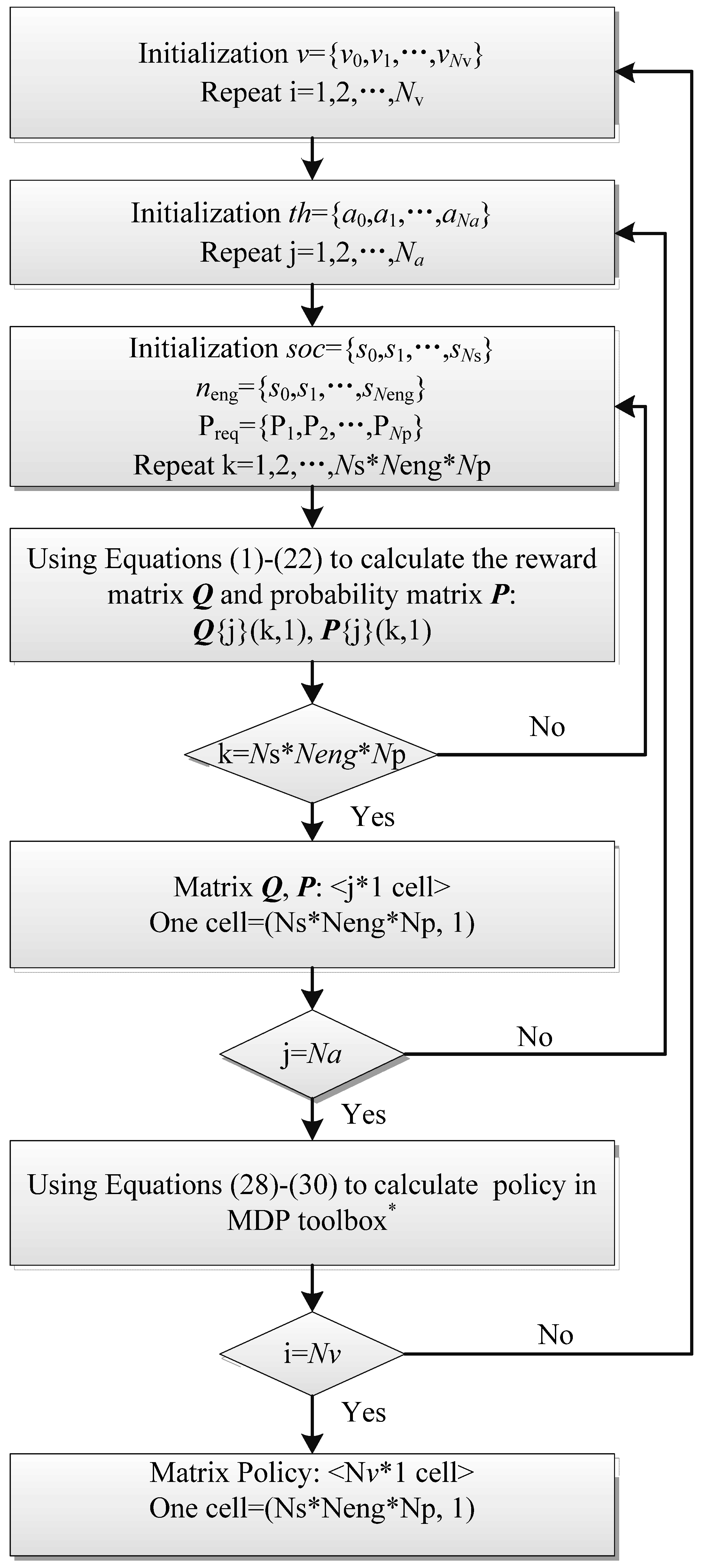
3.2. Q-Learning and Dyna Algorithms
4. Results and Discussion
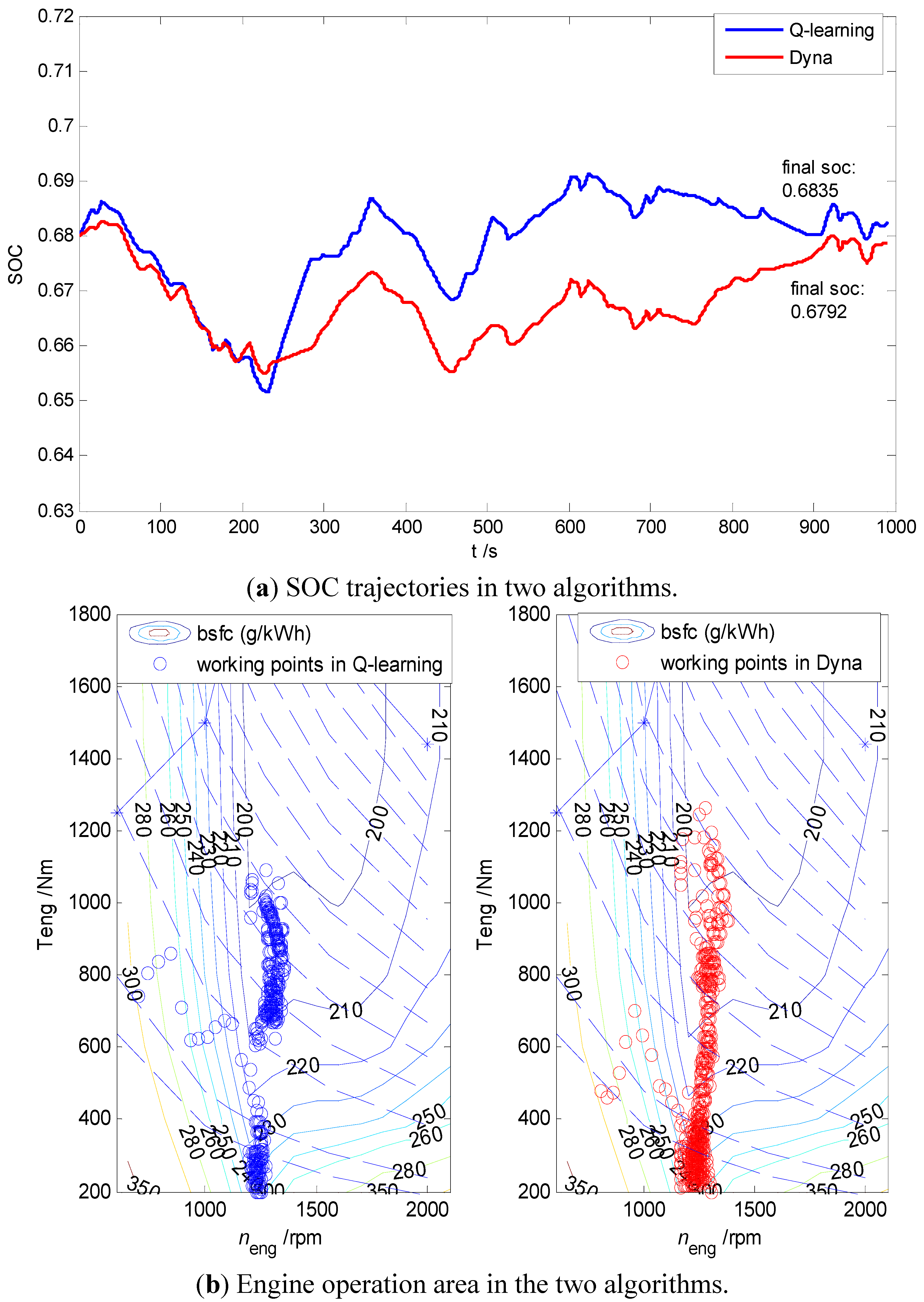
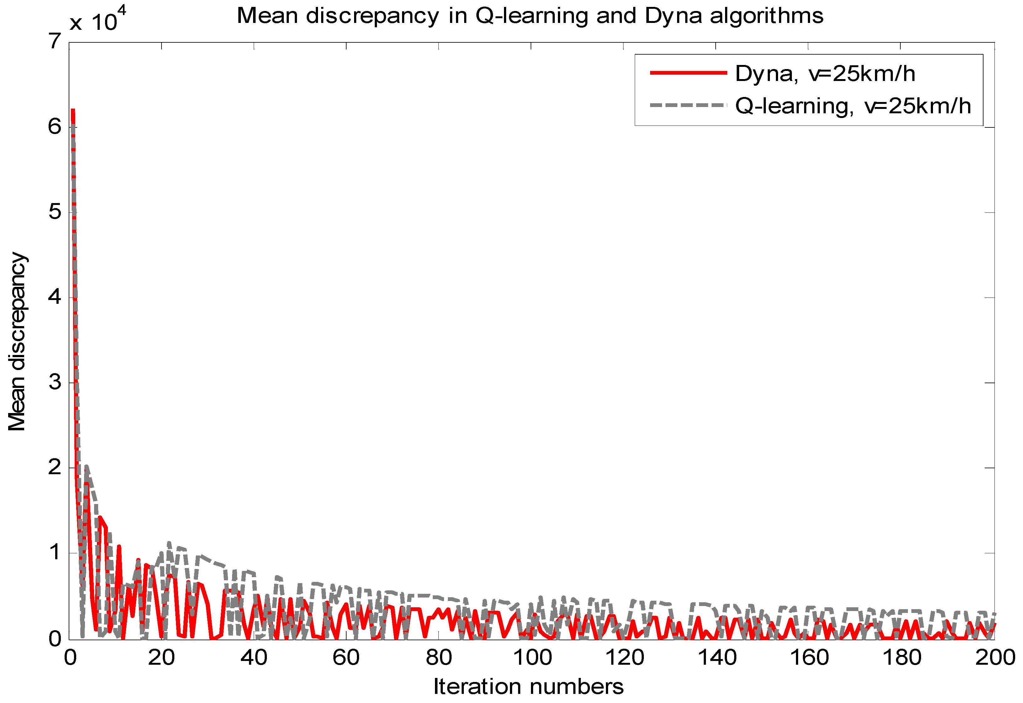
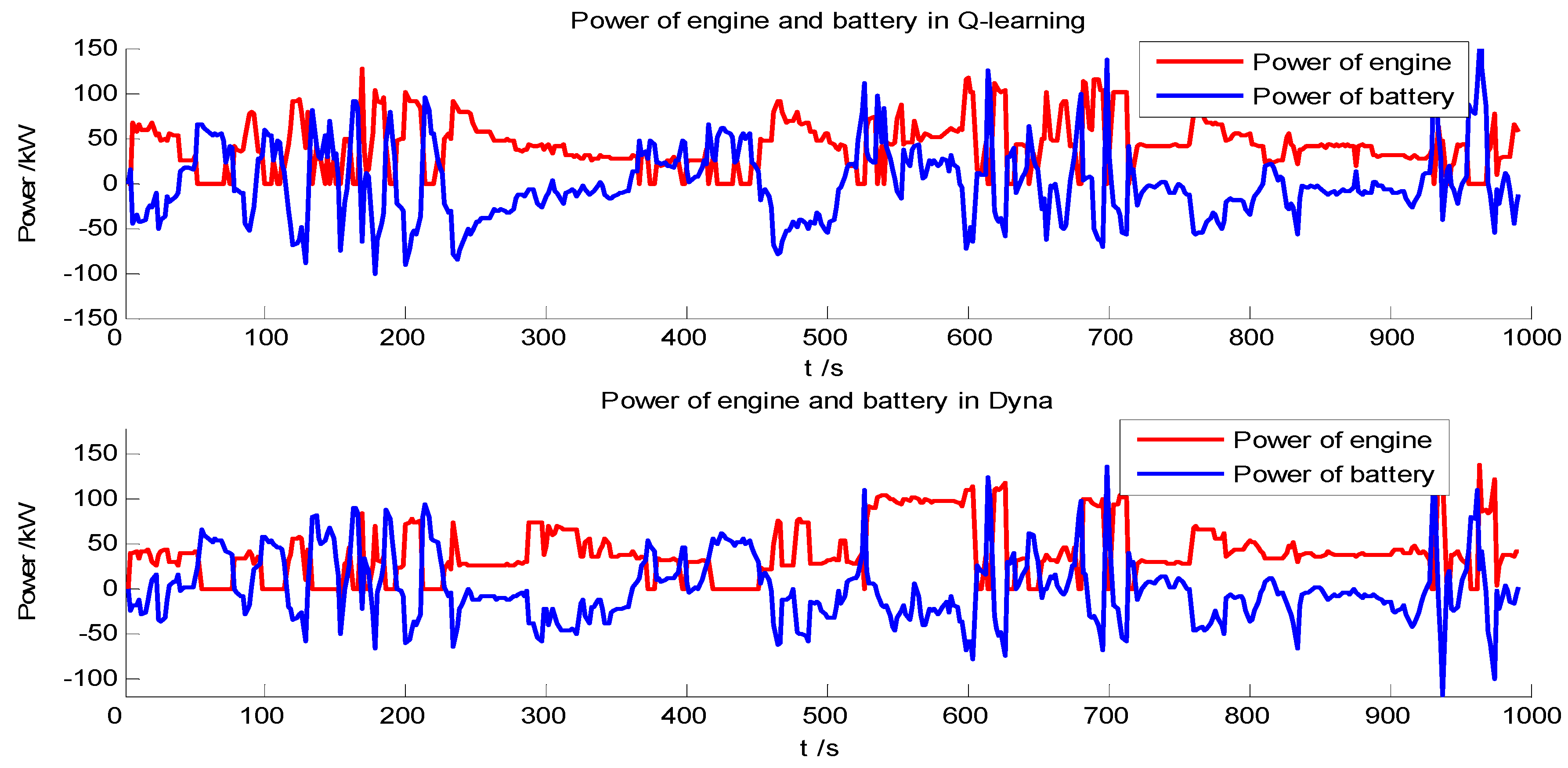
4.1. Comparison between the Q-Learning and Dyna Algorithm


| Algorithm | Fuel Consumption (g) | Relative Increase (%) |
|---|---|---|
| Dyna | 2847 | − |
| Q-learning | 2896 | 1.72 |
| Algorithms | Q-learning | Dyna |
|---|---|---|
| Time a (h) | 3 | 7 |
4.2. Comparative Analysis of the Results of Dyna Algorithm, SDP, and DP
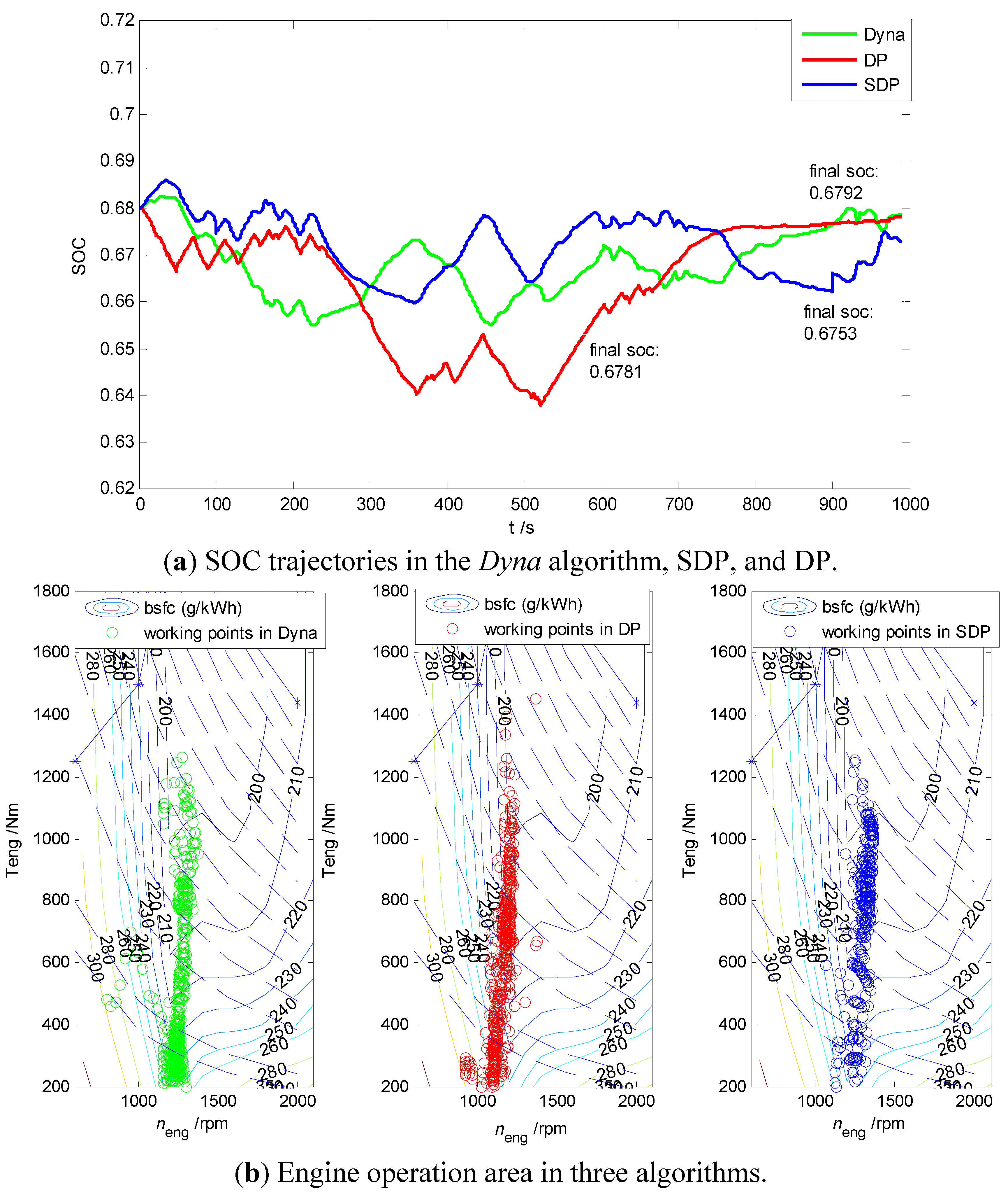
| Algorithm | Fuel Consumption (g) | Relative Increase (%) |
|---|---|---|
| DP | 2847 | ― |
| Dyna | 2853 | 0.21 |
| SDP | 2925 | 2.74 |
| Algorithms | DP | Dyna | SDP |
|---|---|---|---|
| Time a (h) | 2 | 7 | 12 |
5. Conclusions
Acknowledgments
Author Contributions
Conflicts of Interest
References
- Serrao, L.; Onori, S.; Rizzoni, G. A Comparative Analysis of Energy Management Strategies for Hybrid Electric Vehicles. J. Dyn. Syst. Meas. Control 2011, 133, 031012:1–031012:9. [Google Scholar] [CrossRef]
- Lin, C.C.; Kang, J.M.; Grizzle, J.W.; Peng, H. Energy Management Strategy for a Parallel Hybrid Electric Truck. In Proceedings of the American Control Conference 2001, Arlington, VA, USA, 25–27 June 2001; Volume 4, pp. 2878–2883.
- Zou, Y.; Liu, T.; Sun, F.C.; Peng, H. Comparative study of dynamic programming and pontryagin’s minimum principle on energy management for a parallel hybrid electric vehicle. Energies 2013, 6, 2305–2318. [Google Scholar]
- Zou, Y.; Sun, F.C.; Hu, X.S.; Guzzella, L.; Peng, H. Combined optimal sizing and control for a hybrid tracked vehicle. Energies 2012, 5, 4697–4710. [Google Scholar] [CrossRef]
- Sundstrom, O.; Ambuhl, D.; Guzzella, L. On implementation of dynamic programming for optimal control problems with final state constraints. Oil Gas Sci. Technol. 2009, 65, 91–102. [Google Scholar] [CrossRef]
- Johannesson, L.; Åsbogård, M.; Egardt, B. Assessing the potential of predictive control for hybrid vehicle powertrains using stochastic dynamic programming. IEEE Trans. Intell. Transp. Syst. 2007, 8, 71–83. [Google Scholar] [CrossRef]
- Tate, E.; Grizzle, J.; Peng, H. Shortest path stochastic control for hybrid electric vehicles. Int. J. Robust Nonlinear Control 2008, 18, 1409–1429. [Google Scholar] [CrossRef]
- Kim, N.; Cha, S.; Peng, H. Optimal control of hybrid electric vehicles based on Pontryagin’s minimum principle. IEEE Trans. Control Syst. Technol. 2011, 19, 1279–1287. [Google Scholar]
- Delprat, S.; Lauber, J.; Marie, T.; Rimaux, J. Control of a paralleled hybrid powertrain: Optimal control. IEEE Trans. Veh. Technol. 2004, 53, 872–881. [Google Scholar] [CrossRef]
- Nüesch, T.; Cerofolini, A.; Mancini, G.; Guzzella, L. Equivalent consumption minimization strategy for the control of real driving NOx emissions of a diesel hybrid electric vehicle. Energies 2014, 7, 3148–3178. [Google Scholar] [CrossRef]
- Musardo, C.; Rizzoni, G.; Guezennec, Y.; Staccia, B. A-ECMS: An adaptive algorithm for hybrid electric vehicle energy management. Eur. J. Control 2005, 11, 509–524. [Google Scholar] [CrossRef]
- Sciarretta, A.; Back, M.; Guzzella, L. Optimal control of paralleled hybrid electric vehicles. IEEE Trans. Control Syst. Technol. 2004, 12, 352–363. [Google Scholar] [CrossRef]
- Vu, T.V.; Chen, C.K.; Hung, C.W. A model predictive control approach for fuel economy improvement of a series hydraulic hybrid vehicle. Energies 2014, 7, 7017–7040. [Google Scholar] [CrossRef]
- Nüesch, T.; Elbert, P.; Guzzella, L. Convex optimization for the energy management of hybrid electric vehicles considering engine start and gearshift costs. Energies 2014, 7, 834–856. [Google Scholar] [CrossRef]
- Gao, B.T.; Zhang, W.H.; Tang, Y.; Hu, M.J.; Zhu, M.C.; Zhan, H.Y. Game-theoretic energy management for residential users with dischargeable plug-in electric vehicles. Energies 2014, 7, 7499–7518. [Google Scholar] [CrossRef]
- Sutton, R.S.; Barto, A.G. Reinforcement Learning: An Introduction; The MIT Press: Cambridge, MA, USA; London, UK, 2005; pp. 140–300. [Google Scholar]
- Hester, T.; Quinlan, M.; Stone, P. RTMBA: A real-time model-based reinforcement learning architecture for robot control. In Proceedings of the 2012 IEEE International Conference on Robotics and Automation (ICRA), Saint Paul, MN, USA, 14–18 May 2012; pp. 85–90.
- Degris, T.; Pilarski, P.M.; Sutton, R.S. Model-free reinforcement learning with continuous action in practice. In Proceedings of the 2012 American Control Conference, Montreal, QC, Canada, 27–29 June 2012; pp. 2177–2182.
- Perron, J.; Moulin, B.; Berger, J. A hybrid approach based on multi-agent geo simulation and reinforcement learning to solve a UAV patrolling problem. In Proceedings of the Winter Simulation Conference, Austin, TX, USA, 7–10 December 2008; pp. 1259–1267.
- Hsu, R.C.; Liu, C.T.; Chan, D.Y. A reinforcement-learning-based assisted power management with QoR provisioning for human–electric hybrid bicycle. IEEE Trans. Ind. Electron. 2012, 59, 3350–3359. [Google Scholar] [CrossRef]
- Abdelsalam, A.A.; Cui, S.M. A fuzzy logic global power management strategy for hybrid electric vehicles based on a permanent magnet electric variable transmission. Energies 2012, 5, 1175–1198. [Google Scholar] [CrossRef]
- Langari, R.; Won, J.S. Intelligent energy management agent for a parallel hybrid vehicle—Part I: System architecture and design of the driving situation identification process. IEEE Trans. Veh. Technol. 2005, 54, 925–934. [Google Scholar] [CrossRef]
- Guo, J.G.; Jian, X.P.; Lin, G.Y. Performance evaluation of an anti-lock braking system for electric vehicles with a fuzzy sliding mode controller. Energies 2014, 5, 6459–6476. [Google Scholar] [CrossRef]
- Lin, C.C.; Peng, H.; Grizzle, J.W. A stochastic control strategy for hybrid electric vehicles. In Proceedings of the American Control Conference, Boston, MA, USA, 30 June–2 July 2004; pp. 4710–4715.
- Dai, J. Isolated word recognition using Markov chain models. IEEE Trans. Speech Audio Proc. 1995, 3, 458–463. [Google Scholar]
- Brazdil, T.; Chatterjee, K.; Chmelik, M.; Forejt, V.; Kretinsky, J.; Kwiatkowsha, M.; Parker, D.; Ujma, M. Verification of markov decision processes using learning algorithms. Logic Comput. Sci. 2014, 2, 4–18. [Google Scholar]
- Chades, I.; Chapron, G.; Cros, M.J. Markov Decision Processes Toolbox, Version 4.0.2. Available online: http://cran.r-project.org/web/packages/MDPtoolbox/ (accessed on 22 July 2014).
- Kaelbling, L.P.; Littman, M.L.; Moore, A.W. Reinforcement learning: A survey. Artif. Intell. Res. 1996, 4, 237–285. [Google Scholar]
- Zou, Z.Y.; Xu, J.; Mi, C.; Cao, B.G. Evaluation of model based state of charge estimation methods for lithium-Ion batteries. Energies 2014, 7, 5065–5082. [Google Scholar] [CrossRef]
- Jimenez, F.; Cabrera-Montiel, W. System for Road Vehicle Energy Optimization Using Real Time Road and Traffic Information. Energies 2014, 7, 3576–3598. [Google Scholar] [CrossRef]
- Filev, D.P.; Kolmanovsky, I. Generalized markov models for real-time modeling of continuous systems. IEEE Trans. Fuzzy Syst. 2014, 22, 983–998. [Google Scholar] [CrossRef]
- Di Cairano, S.; Bernardini, D.; Bernardini, D.; Bemporad, A.; Kolmanovsky, I.V. Stochastic MPC with Learning for Driver-Predictive Vehicle Control and its Application to HEV Energy Management. IEEE Trans. Cont. Syst. Technol. 2015, 22, 1018–1030. [Google Scholar] [CrossRef]
© 2015 by the authors; licensee MDPI, Basel, Switzerland. This article is an open access article distributed under the terms and conditions of the Creative Commons Attribution license (http://creativecommons.org/licenses/by/4.0/).
Share and Cite
Liu, T.; Zou, Y.; Liu, D.; Sun, F. Reinforcement Learning–Based Energy Management Strategy for a Hybrid Electric Tracked Vehicle. Energies 2015, 8, 7243-7260. https://doi.org/10.3390/en8077243
Liu T, Zou Y, Liu D, Sun F. Reinforcement Learning–Based Energy Management Strategy for a Hybrid Electric Tracked Vehicle. Energies. 2015; 8(7):7243-7260. https://doi.org/10.3390/en8077243
Chicago/Turabian StyleLiu, Teng, Yuan Zou, Dexing Liu, and Fengchun Sun. 2015. "Reinforcement Learning–Based Energy Management Strategy for a Hybrid Electric Tracked Vehicle" Energies 8, no. 7: 7243-7260. https://doi.org/10.3390/en8077243
APA StyleLiu, T., Zou, Y., Liu, D., & Sun, F. (2015). Reinforcement Learning–Based Energy Management Strategy for a Hybrid Electric Tracked Vehicle. Energies, 8(7), 7243-7260. https://doi.org/10.3390/en8077243