Credibility Theory-Based Available Transfer Capability Assessment

Abstract

Since the development of large scale power grid interconnections and power markets, research on available transfer capability (ATC) has attracted great attention. The challenges for accurate assessment of ATC originate from the numerous uncertainties in electricity generation, transmission, distribution and utilization sectors. Power system uncertainties can be mainly described as two types: randomness and fuzziness. However, the traditional transmission reliability margin (TRM) approach only considers randomness. Based on credibility theory, this paper firstly built models of generators, transmission lines and loads according to their features of both randomness and fuzziness. Then a random fuzzy simulation is applied, along with a novel method proposed for ATC assessment, in which both randomness and fuzziness are considered. The bootstrap method and multi-core parallel computing technique are introduced to enhance the processing speed. By implementing simulation for the IEEE-30-bus system and a real-life system located in Northwest China, the viability of the models and the proposed method is verified.

1. Introduction

Available transfer capability (ATC) expresses a measure of transfer capability remaining in a physical transmission network for further commercial activity over and above already committed uses [1]. It is not only an important technical index for measuring the stability margin of the power grid, but also a useful tool for guiding transactions and market planning in the power market. Therefore it is very important to correctly assess ATC between different areas. The modern power system is a large scale dynamic system. As power systems have grown, their operation has become more complex with the introduction of more outside interferences. As a result, uncertainty factors are becoming prevalent in the assessment of ATC. Moreover, power industry reforms necessarily lead to an increasing number of market participants, which greatly changes the trade mode and operation control. These also produce more uncertainties in the ATC assessment. Hence how to correctly describe and fully consider uncertainties is the key issue of ATC assessment [2].

The uncertainty represents the unknown state of the future. The power system uncertainties mainly come from equipment outages, load changes, operation modes and so on. The concept of transmission reliability margin (TRM) was introduced by the North American Electric Reliability Council (NERC) in 1996 to consider the impacts of these uncertainties on ATC. It represents the amount of transmission transfer capability needed to ensure that the interconnected transmission network is secure under a reasonable range of uncertainties under the system conditions. Currently two approaches are usually used to deal with TRM [3,4]: (1) take a fixed percentage of the total transfer capability (TTC), such as 4% of TTC or reduce the limit of equipment parameters by a certain percent. This approach is easy to carry out but it is difficult to choose a reasonable percentage, and a rough result is achieved; (2) use stochastic methods [5,6] whereby according to the random distributions of the uncertainties, the ATC calculations are repeated using different uncertainty parameters, then the ATC distribution can be obtained, and TRM is the difference between the maximum value and the expected value of this ATC distribution. This type of approach only considers the power system randomness. However, power systems actually contain two types of uncertainties—randomness and fuzziness—and there a lot of uncertainties in power systems with both random and fuzzy features. For example, the failure of a generator is random, while its available output is fuzzy; similarly a transmission line failure is a random event, and its failure rate which is affected by many factors that embody fuzziness; the probability distribution of a load is random, but its distribution variance is fuzzy. Both randomness and fuzziness are important characteristics of the uncertainties in power systems, and each has great effects. Therefore, how to comprehensively describe these uncertainty features is an important potential difficulty in ATC assessment, but with little achievement reported in the state-of-the-art literature.

Although research on comprehensive evaluations that consider both randomness and fuzziness simultaneously has been constantly tried, a series of problems that cannot be easily overcome have made progress in this field very slow. The biggest obstacle is that there was no complete theory to support it in the field of basic mathematics until the credibility measure was proposed by Liu in 2002 and then the credibility theory was established [7,8,9,10,11]. The theory puts forward the concept of the opportunity space and mixed variables, allowing a comprehensive evaluation method for randomness and fuzziness to be set up.

Now the credibility theory has been applied to power systems [12,13,14]. According to the two-fold uncertainty combining randomness and fuzziness in power system operations, a novel operation risk assessment method based on credibility theory is presented; the expected value and the average chance measure of random fuzzy variables was used to build on index of operation risk in [12]. Considering both the randomness of force outage rates and the fuzziness of hydro energy, a comprehensive model of hydro-thermal generator maintenance scheduling based on credibility theory was established in [13]. In [14] a new methodological framework with chance-constrained random fuzzy programming, which evaluated the randomness of the forecasted load, the fuzziness of rivals’ biddings strategies and price-demand elasticity, was developed for building optimal bidding strategies for generation companies with uncertainty theory-based risk management taken into account was presented and a hybrid intelligent algorithm with combined random fuzzy simulation, artificial neural network and genetic algorithm was proposed to solve the random fuzzy programming problem.

However, very limited work has considered both the randomness and fuzziness that actually coexist in the assessment of ATC. A chance-constrained random fuzzy programming method to consider TRM was introduced in [15], but it still treated the important factors which affected the reliable of transmission as random variables or ones that obeyed a normal distribution. Comprehensive research which considers both randomness and fuzziness at the same time has not been done. This paper builds for the first time comprehensive models of generators, transmission lines and loads according to their randomness and fuzziness features. No stochastic or possibilistic programming can single-handedly deal with these complex uncertainty models, therefore a random fuzzy simulation is also introduced for the first time to the assessment of ATC. A novel assessment method is proposed based on credibility theory. The bootstrap method and multi-core parallel computing technique are used to enhance the speed of processing. As the main contribution of this paper, the concept and approach have been tested on the IEEE-30-bus system and a real-life system.

The paper is organized as follows: the basic concepts of credibility theory with some application examples concerning power systems are introduced in Section 2, which includes four axioms, credibility measure, random fuzzy variables and their expected values and variances In Section 3. some subjects such as random fuzzy modeling of the main uncertainty factors, the ATC calculation model and the assessment indices, bootstrap method and multi-core parallel computing technique, and the ATC assessment of random fuzzy simulation are presented. A numerical simulation with the IEEE 30 bus system and an actual Chinese system aregiven to demonstrate the feasibility of the proposed models and methods in Section 4, followed by our conclusions in Section 5.

2. Credibility Theory

There are a large amount of uncertainties in the real world. They could be in results, categories, or their combinations. The result uncertainties are represented by probability methods. The corresponding theory and methods have already been well developed, whereas some other uncertainties affected by the weather, the environment and operational conditions are changing from time to time under real-time conditions. In other words, they may vary significantly under different conditions, so it is difficult to simply quantify the co-relationship among these uncertainties by randomness. Fortunately, they can be described using fuzzy words based on experienced operators’ judgment (such as “most adverse”, “fairly adverse” or “less adverse”, etc.), which can be modeled using a fuzzy membership function [9,16,17,18,19]. Fuzzy theory and its methods have been popular yet challenging for many years. In 1975 Kaufmann proposed the concept of fuzzy variables for the first time [20]. Then in 1978 Zadeh put forward the possibility theory which depicted the possibility of occurrence of fuzzy events [21], and laid an important foundation for the development of fuzzy theory, although at that time incompatible counter-examples in fuzzy theory still existed, and fuzzy theory had not been verified axiomatically. The axiomatic system of fuzzy theory was finally verified by the Chinese mathematician Baoding Liu in the 21st century. Since then credibility theory was developed and now offers a strict theoretical foundation for modeling and solving problems with randomness and fuzziness.

2.1. Basic Concept

The following four axioms are the base of fuzzy theory. Let Θ be a non-empty set and ϕ an empty set. P(Θ) is the power set of Θ, ∧ is the minimum operator and sup is the supremum operator. The possibility measure of the event A is defined as P_os{A}:

Axiom 1: $P_{os}\left\{\mathrm{\Theta }\right\}=1$.

Axiom 2: $P_{os}\left\{\varphi \right\}=0$.

Axiom 3: for any set {A_i} in P(Θ).

$P_{os}\left\{{\displaystyle {\cup }_i{A}_i}\right\}={\sup }_i{P}_{os}\left\{A_i\right\}$.

Axiom 4: if Θ_I is a non-empty set, Posi{·}, i=1,2,…,n meets the first three axioms, and Θ=Θ₁×Θ₂×…×Θ_n, for any set A∈P(Θ), $P_{os}\{A\}=\underset{({\mathrm{\theta }}_1,{\mathrm{\theta }}_2,\cdots ,{\mathrm{\theta }}_n)\in A}{\sup }{P}_{os1}\{{\mathrm{\theta }}_1\}\wedge P_{os2}\{{\mathrm{\theta }}_2\}\wedge \cdots \wedge P_{osn}\{{\mathrm{\theta }}_n\}$.

Definition 1: if P_OS meets the first three axioms, P_OS is defined as the possibility measure. (Θ, P(Θ), P_OS) is a possibility space. If A^c is the complement of A, the necessity measure N_ec is defined as N_ec{A}=1 − P_os{A^c}. Obviously, P_OS and N_ec are one pair of dual measures, so the credibility measure is defined as follows:

$$C_r\{A\}=\frac{1}{2}(P_{os}\{A\}+N_{ec}\{A\})$$

(1)

When the possibility measure of a fuzzy event is 1, the event may not exist, but when the necessity measure of a fuzzy event is 0, this event may still exist. However, the fuzzy event must exist if its credibility is 1, otherwise it does not exist if its credibility is 0. The basis of credibility theory is the definition of a credibility measure, whose position equals one of the probability measures in probability theory.

Definition 2: A fuzzy variable ξ is a function from the possibility space (Θ, P(Θ), P_OS) to the real line R. The triangle fuzzy variable and the trapezoidal fuzzy variable are commonly used ones.

Definition 3: Let ξ be a fuzzy variable in a possibility space (Θ, P(Θ), P_OS), the membership function of ξ is:

$$\mathrm{\mu }(x)=P_{os}\{\mathrm{\theta }\in \mathrm{\Theta }|\mathrm{\xi }(\mathrm{\theta })=x\},x\in R$$

(2)

Through the above definition the following inversion formula can be proved: for any set B of real numbers, we have:

$$C_r\{\mathrm{\xi }\in B\}=(\underset{x\in B}{\sup }\mathrm{\mu }(x)+1-\underset{x\in B^c}{\sup }\mu (x))/2$$

(3)

Example 1: The available output of a generator has an uncertain feature. Especially when green energy forms, such as hydropower, wind power, solar power and so on are vigorously developed, its unreliable forecasting characteristics and the weather dependency will increase the uncertainties. It is very difficult to get the exact output of a generator, but we can roughly use a triangle fuzzy variable ξ_G to represent its available output. Suppose the available output ξ_G = (35, 50, 55) MW, we have the credibility measure of ξ_G:

$$C_r\{{\mathrm{\xi }}_G\ge r\}=\{\begin{array}{cc}\hfill 1,& r\le 35\hfill \\ \hfill \frac{65-r}{30},& 35<r\le 50\hfill \\ \hfill \frac{55-r}{10},& 50<r\le 55\hfill \\ \hfill 0,& 55<r\hfill \end{array}$$

Definition 4: Let ξ be a fuzzy variable. The expected value of ξ is defined as:

$$E_{fuz}[\mathrm{\xi }]={\displaystyle {\int }_0^{\infty }{C}_r\{\mathrm{\xi }\ge r\}dr}-{\displaystyle {\int }_{-\infty }^0{C}_r\{\mathrm{\xi }\le r\}dr}$$

(4)

To avoid possible occurrence of ∞–∞, at least one of the two integrals is limited in the above Equation (4).

Example 2: The expected value of a triangle fuzzy variable (a, b, c) can be obtained:

$$E_{fuz}[\mathrm{\xi }]=(a+2b+c)/4$$

The expected value of a trapezoidal variable (a, b, c, d) is:

$$E_{fuz}[\mathrm{\xi }]=(a+b+c+d)/4$$

2.2. Random Fuzzy Variable

Definition 5: A random fuzzy variable ε is a function from the possibility space (Θ, P(Θ), P_OS) to the set of random variables.

Example 3: There are two states of a generator: on state, and off fault state. They are random, while its available output is fuzzy, so the state of a generator can be represented using a two-point distribution random fuzzy variable ε. For instance, it can be represented as P_pro,G(ε = ξ_G) = 0.99, P_pro,G(ε = 0) = 0.01. ξ_G is a triangle fuzzy variable as defined in Example 1.

Definition 6: Let ε be a random fuzzy variable, the expected value of ε is defined as:

$$\begin{array}{ll}{E}_{pro-fuz}[\epsilon ]& ={\displaystyle {\int }_0^{\infty }{C}_r\{\mathrm{\theta }\in \mathrm{\Theta }|E[\epsilon (\mathrm{\theta })]\ge r\}dr}\\ & -{\displaystyle {\int }_{-\infty }^0{C}_r\{\mathrm{\theta }\in \mathrm{\Theta }|E[\epsilon (\mathrm{\theta })]\le r\}dr}\end{array}$$

(5)

Also to avoid the situation of ∞–∞, at least one of the two integrals is limited in Equation (5).

Definition 7: Let ε be a random fuzzy variable and it has a limited expected value. The variance of ε is defined as:

V[ε] = E[(ε − E[ε])²]

(6)

Example 4: The random fuzzy variable ε(θ) defined in Example 3 is a two-point distribution random variable for each θ, where θ is a sample from a possibility space. The expected value of ε(θ) is:

$$E_{pro}[\epsilon (\mathrm{\theta })]=0.99{\mathrm{\xi }}_G(\mathrm{\theta })$$

According to Definition 4, the expected value of a two-point distribution random fuzzy variable ε is:

$$\begin{array}{ll}{E}_{pro-fuz}(\epsilon )& =0.99E_{fuz}[{\mathrm{\xi }}_G]\\ & =0.99\times ((35+2\times 50+55)/4)=47.025\end{array}$$

3. Credibility Theory-Based ATC Assessment Approach

3.1. Modeling Uncertainties in ATC Calculation

The assessment to ATC involves many uncertain factors, such as those in generation scheduling, in load forecasting and so on. Compared with previous methods, this paper comprehensively considers three main uncertain factors: random fuzzy models of generators, transmission lines and loads (to consider faults and fluctuations). It is worth noting that other uncertainty factors included in ATC calculation can also be treated in a similar way using credibility theory, and are potentially applicable to enrich and make the ATC calculation flexible by considering more factors. The corresponding random fuzzy models are built up as follows:

(1) For generators under the combined effects of the internal and external factors, there are two common states that are on-state and off-state. They are subject to a two-point random distribution according to the forced outage rate which comes from the statistics. When the generator is on-state, its output is greatly affected by many factors such as coal quality, reserve requirements, weather conditions and so on, so for a specific generator, its output is not an exact value and may vary significantly under different conditions. Although the equivalent forced outage rate [22] considers the conditions of outage and output reduction, it could not involve the conditions of overload operation, and since it depends on the statistics of a large number of historical data and the complex calculations, its value is hard to get for each generator in practical systems, especially for a newly installed generator, while through the simple fuzzy membership function of generator available output, which needs few parameters, the complex conditions can be described well by fuzzy variables, thus, the states of generators are suitable for being represented as discrete random fuzzy variables ε_G with two-point distribution:

$$\{\begin{array}{l}{P}_{pro,G}({\mathrm{\epsilon }}_G)=\{\begin{array}{c}1-{\mathrm{\lambda }}_G,{\mathrm{\epsilon }}_G={\mathrm{\xi }}_G\\ {\mathrm{\lambda }}_G,{\mathrm{\epsilon }}_G=0\end{array}\\ F_{fuz,G}({\mathrm{\xi }}_G)=\{\begin{array}{cc}\frac{{\mathrm{\xi }}_G-a_{G,L}}{a_{G,M}-a_{G,L}},& a_{G,L}\le {\mathrm{\xi }}_G\le a_{G,M}\\ \frac{a_{G,H}-{\mathrm{\xi }}_G}{a_{G,H}-a_{G,M}},& a_{G,M}\le {\mathrm{\xi }}_G\le a_{G,H}\\ 0,& Other\end{array}\end{array}$$

(7)

where P_pro,G is the state occurrence probability of the generator; ε_G = ξ_G refers to the normal on-state, and ε_G = 0 is the off-state; the triangle fuzzy variable ξ_G is used to represents the fuzzy available output of a generator, and F_fuz,G represents its membership function; a_G,L, a_G,M, a_G,H are the minimum possible value, the most likely possible value and the maximum possible value of ξ_G, respectively. In this paper triangle fuzzy variables are used to represent the fuzzy states of the generator, transmission line and load, but other types of fuzzy variables such as trapezoidal fuzzy variables, can also be used according to specific conditions.

(2) The state of transmission line also obeys a two-point random distribution according to its failure rate. Conventionally, the longer the transmission line, the higher the failure rate in the same area and for the same voltage level, but practical experience indicates that the occurrence of faults in outdoor transmission lines is affected by many factors, including the weather conditions. Therefore the failure rate is a fuzzy value for a specific transmission line, which changes with the weather conditions and the area considered [23]. The method presented in [24] where the failure rate can be modified through probability statistics is hard to apply in practical systems, so in order to comprehensively describe randomness and fuzziness on the whole, it is proper to representthe states of transmission lines as random fuzzy variables ε_B as follows:

$$\{\begin{array}{l}{P}_{pro,B}({\mathrm{\epsilon }}_B)=\{\begin{array}{c}1-{\mathrm{\xi }}_B,{\mathrm{\epsilon }}_B=1\\ {\mathrm{\xi }}_B,{\mathrm{\epsilon }}_B=0\end{array}\\ F_{fuz,B}({\mathrm{\xi }}_B)=\{\begin{array}{cc}\frac{{\mathrm{\xi }}_B-a_{B,L}}{a_{B,M}-a_{B,L}},& a_{B,L}\le {\mathrm{\xi }}_B\le a_{B,M}\\ \frac{a_{B,H}-{\mathrm{\xi }}_B}{a_{B,H}-a_{B,M}},& a_{B,M}\le {\mathrm{\xi }}_B\le a_{B,H}\\ 0,& Otherwise\end{array}\end{array}$$

(8)

where P_pro,B is the state occurrence probability of the transmission line; ε_B = 1 expresses the normal on-state, and ε_B = 0 is the off-state; the triangle fuzzy variable ξ_B is used to represents the fuzzy failure rate of the transmission line, and F_fuz,B represents its membership function; a_B,L, a_B,M, a_B,H are the minimum possible value, the most likely possible value and the maximum possible value of ξ_B, respectively.

(3) As a main uncertainty factor in ATC assessment, the fluctuation of nodal load is considered to obey a normal distribution N(β_L, σ_L) in traditional methods. Here the parameter β_L is the expected value of the distribution, which usually takes the predicted value of the nodal load. The parameter σ_L is the variance of the distribution, which shows the degree of deviation between the real value of the load and the forecasted one, and is usually determined according to the operator’s experience. Actually, σ_L is not a fixed value, but a fuzzy one, so the fluctuation of nodal load has both randomness and fuzziness features, so the random fuzzy load ε_L is represented as follows:

$$\{\begin{array}{l}{\mathrm{\epsilon }}_L~N({\mathrm{\beta }}_L,{\mathrm{\xi }}_L)\\ F_{fuz,L}({\mathrm{\xi }}_L)=\{\begin{array}{cc}\frac{{\mathrm{\xi }}_L-a_{L,L}}{a_{L,M}-a_{L,L}},& a_{L,L}\le {\mathrm{\xi }}_L\le a_{L,M}\\ \frac{a_{L,H}-{\mathrm{\xi }}_L}{a_{L,H}-a_{L,M}},& a_{L,M}\le {\mathrm{\xi }}_L\le a_{L,H}\\ 0,& Otherwise\end{array}\end{array}$$

(9)

where the triangle fuzzy variable ξ_L is used to represents the fuzzy variance of a nodal load, and F_fuz,L represents its membership function; a_L,L, a_L,M, a_L,H are the minimum possible value, the most likely possible value and the maximum possible value of ξ_L, respectively.

3.2. ATC Calculation Model

An improved repeated power flow method is adopted to calculate the ATC for each simulation state in this paper. The method starts from an initial operation point, then increases the load powers in the receiving area according to their proportion of the initial power, at the same time increases the generators’ power outputs in the sending area according to their generation cost, until a certain constraint hits its limit, such as the node voltage exceeding its operating limit, or the transmission line being overloaded and so on. The net increase on the researched interface is the ATC of this simulation state. Such a conventional repeated power flow method only pays attention to system safety, but neglects the economics, so this paper introduces the optimal power flow [25,26] as shown in Equation (10) into every power flow computation of the repeated power flow method to comprehensively consider both safety and economy; it can get a more accurate results and better meet the real application needs in the power market:

$$\{\begin{array}{l}\min f\\ s.t.P_g-P_d-V_x{\displaystyle \sum V_y(G_{xy}\cos {\delta }_{xy}+B_{xy}\sin {\delta }_{xy})}=0\\ Q_g-Q_d+V_x{\displaystyle \sum V_y(G_{xy}\cos {\delta }_{xy}-B_{xy}\sin {\delta }_{xy})}=0\\ P_g^{\min }\le P_g\le P_g^{\max }\\ Q_g^{\min }\le Q_g\le Q_g^{\max }\\ V_z^{\min }\le V_z\le V_z^{\max }\\ \left|S_l\right|\le S_l^{\max }\end{array}$$

(10)

where the first two equality constraints are the active and reactive power balance equations and the remaining are the inequality constraints of generator output, node voltage and apparent power of the transmission lines.

3.3. ATC Assessment Indices

In order to accurately assess ATC and make a comparison with different methods, three assessment indices are proposed as follows:

(a)

The expected value of random fuzzy ATC—E_ATC—it comprehensively reflects the ATC of a power system.

$$\begin{array}{l}{E}_{pro-fuzz,\mathrm{ATC}}={\displaystyle {\int }_0^{\infty }{C}_r\{\mathrm{\theta }\in \mathrm{\Theta }|E[{\mathrm{\epsilon }}_{\text{ATC}}(\mathrm{\theta })]\ge r\}dr}\\ -{\displaystyle {\int }_{-\infty }^0{C}_r\{\mathrm{\theta }\in \mathrm{\Theta }|E[{\mathrm{\epsilon }}_{\text{ATC}}(\mathrm{\theta })]\le r\}dr}\end{array}$$

(11)

(b)

The variance of random fuzzy ATC—V_ATC—it expresses the fluctuation of ATC and reflects the impacts of uncertainties on ATC:

$$V_{pro-fuz\text{,ATC}}=E[{({\mathrm{\epsilon }}_{\text{ATC}}-E_{\text{ATC}})}^2]$$

(12)

(c)

Calculation time t: it reflects the efficiency of different ATC calculation approaches under the same initial conditions.

3.4. Parallel Algorithm with Bootstrap Method

The bootstrap method is a statistical analysis method adopted in numerical computation, which was for the first time put forward by Efron at Stanford University [27,28]. It makes full use of the information of samples and can provide an approximate distribution of the unknown parameters in an unknown system directly through (repeated) re-sampling in a small sample set. The bootstrap method is adopted in the random simulation in this paper, and as a result the sample size can be decreased remarkably and the processing speed is enhanced. ATC calculation for each simulation state is a complex nonlinear optimization problem. The primal-dual interior-point algorithm in Matpower4.0b4 [29] is applied to solve the problem, which makes full use of multi-core and multi-threading CPUs by parallel computing.

3.5. Random Fuzzy Simulation Based ATC Assessment

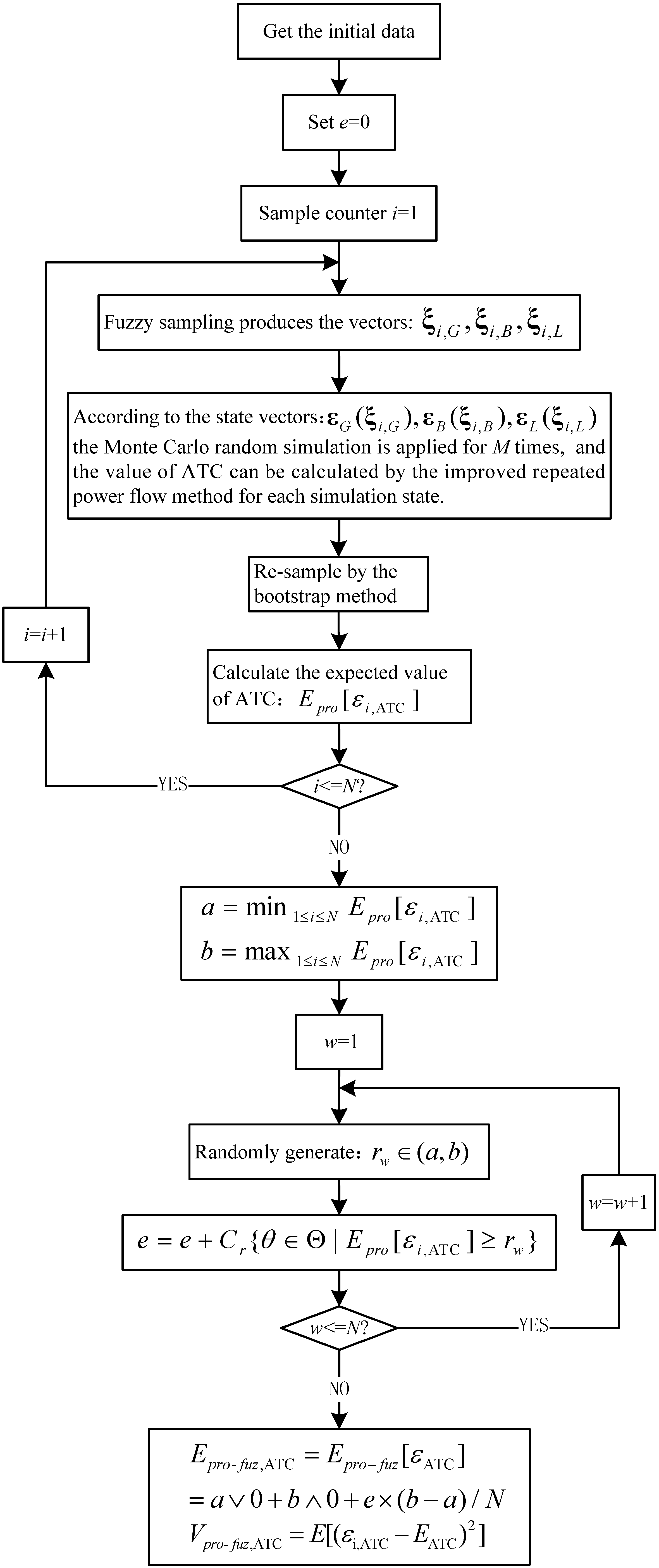
According to the above random fuzzy models of generators, transmission lines and loads, how to simulate these random and fuzzy uncertain factors is the key issue in ATC assessment. Obviously the conventional probability methods are invalid, and these models cannot be directly changed to deterministic equivalence problems, so the random fuzzy simulation is proposed to solve the ATC assessment with randomness and fuzziness. Firstly, according to the above models the fuzzy parameters are sampled, based on each fuzzy sample Monte Carlo random sampling is done for every random parameter, and as a result the possible states are simulated with the comprehensive consideration of both randomness and fuzziness.

Figure 1. The flowchart of ATC assessment.

Figure 1. The flowchart of ATC assessment.

Then the value of ATC for each simulation state is calculated by the improved repeated power flow method. The bootstrap method helps find the random distribution of ATC with fewer calculation results and enhances the processing speed. Lastly the comprehensive assessment indices can be obtained according to the random fuzzy computational framework. Figure 1 illustrates the procedure for assessing ATC. Detailed steps are described as follows:

(1)

Read the initial parameters of generators, transmission lines and loads, build basic system information and set e = 0, i = 1.

(2)

From the set Θ extract a θ_k which meets P_OS{θ_k} ≥ ε (ε is a permissible small value making the sample space be bounded), get the variables of generators, transmission lines and loads, and produce a set of fuzzy sampling vectors: ${\mathrm{\xi }}_{i,G},{\mathrm{\xi }}_{i,B},{\mathrm{\xi }}_{i,L}$.

(3)

According to ${\mathrm{\xi }}_{i,G},{\mathrm{\xi }}_{i,B},{\mathrm{\xi }}_{i,L}$ and the corresponding equipment random parameters, get the system state vectors: ${\epsilon }_G({\mathrm{\xi }}_{i,G}),{\epsilon }_B({\mathrm{\xi }}_{i,B}),{\epsilon }_L({\mathrm{\xi }}_{i,L})$, change the random fuzzy models of generators, transmission lines and loads to the random ones, then the fuzziness is eliminated. Then the Monte Carlo random simulation is applied M times, and the value of ATC can be calculated by the improved repeated power flow method for each simulation state.

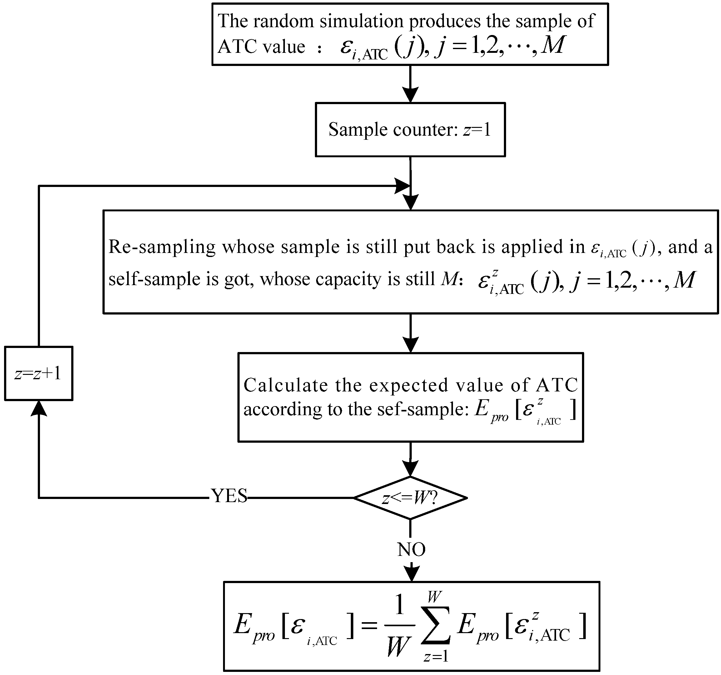
(4)

By the bootstrap method re-sample in the above obtained ATC values, and calculate their expected value of ATC. Figure 2 illustrates the bootstrap method procedure.

(5)

Set sample counter i = i + 1, and repeat (2) to (4) for N times.

(6)

Set a = min_1≤i≤NE_pro[ε_i,ATC], b = max_1≤i≤NE_pro[ε_i,ATC], and loop control variable w = 1.

(7)

From the interval [a, b] randomly generate r_w and calculate $e=e+C_r\{\mathrm{\theta }\in \mathrm{\Theta }|E_{pro}[{\epsilon }_{i,\text{ATC}}]\ge r_w\}$.

(8)

Set w = w + 1, and repeat (7) for N times.

(9)

Lastly calculate the expected value and variance of ATC as follows:

$$E_{pro-fuz\text{,ATC}}=E_{pro-fuz}[{\mathrm{\epsilon }}_{\text{ATC}}]=a\vee 0+b\wedge 0+e\times (b-a)/N, V_{pro-fuz\text{,ATC}}=E[{({\mathrm{\epsilon }}_{\text{i,ATC}}-E_{\text{ATC}})}^2].$$

Figure 2. The flowchart of the bootstrap method.

Figure 2. The flowchart of the bootstrap method.

4. Numerical Example

The simulation uses a Lenovo T400 (CPU: Core2 Duo 2.26 G; RAM: 3 G) laptop as the calculation platform. Matpower4.0b4 which provides the power flow calculation program is adopted as the simulation software under Matlab R2008a. The IEEE-30-bus system and an actual power system of two regions in Northwest China are used to demonstrate applications of the proposed models and algorithm.

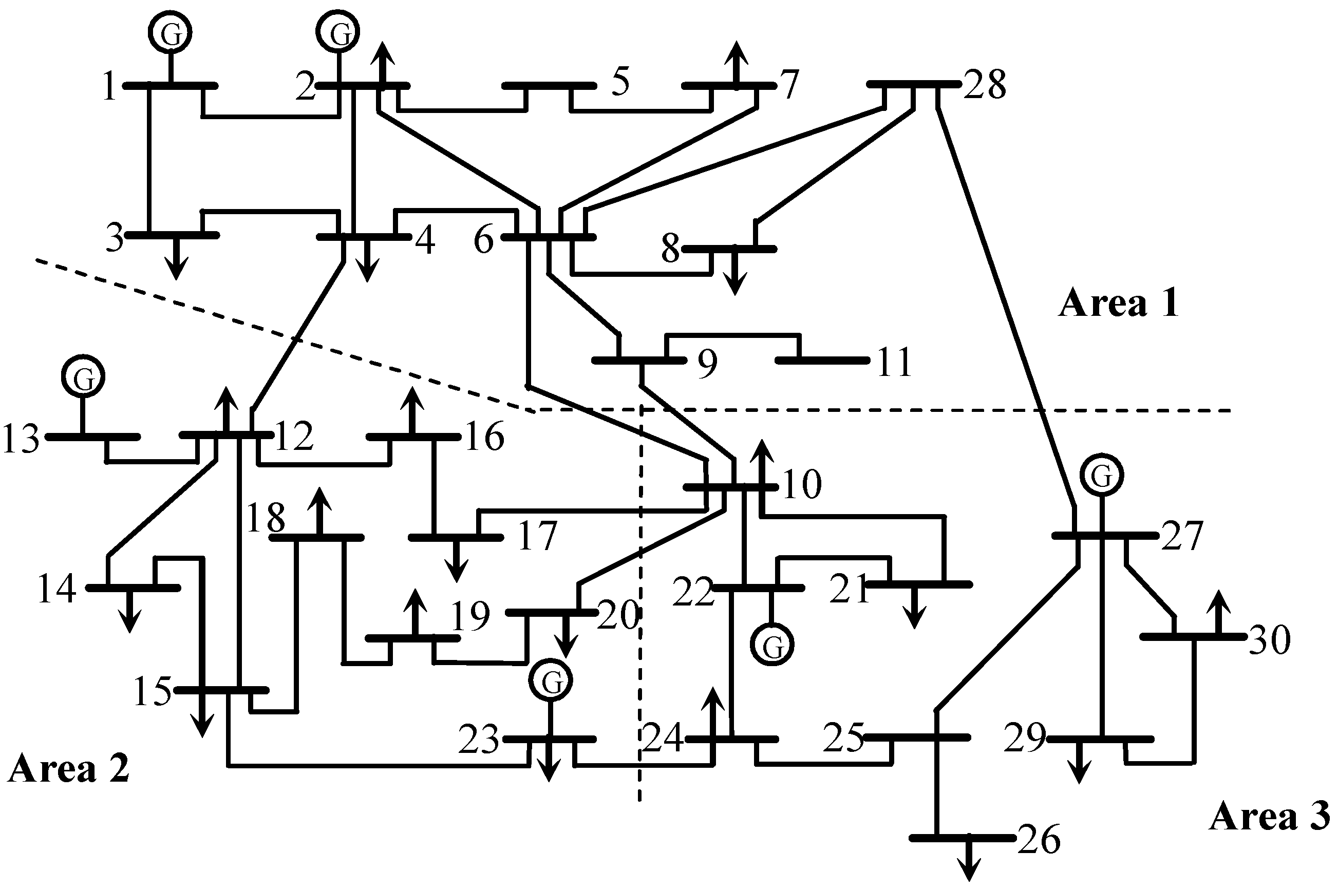
4.1. IEEE-30-bus System

The single line diagram of the IEEE-30-bus system (the base capacity is 100 MVA) is shown in Figure 3. The system has 30 load nodes and 41 transmission lines, divided into three areas. The equipment parameters are given in [30]. This paper focuses on the ATC assessment from Area 1 to Area 2. The parameters of the random fuzzy simulation are set as follows: N = 3000, M = 80, W = 10. The proposed ATC assessment method based on credibility theory is verified in several scenarios. In Part 1, Part 2 and Part 3 only a single random fuzzy factor, such as random fuzzy generators or random fuzzy transmission lines or random fuzzy loads, is considered in each case to reflect its effect on ATC. In Part 4 all the above random fuzzy factors are considered simultaneously to compare the processing efficiency of each one.

Figure 3. IEEE-30-bus system.

Figure 3. IEEE-30-bus system.

Part 1: Compatibility analysis between the proposed approach and the conventional Monte Carlo random simulation.

For Case A to Case F, the parameters of generators, transmission lines and loads are shown in Table 1, and the corresponding assessment results are listed in Table 2, Table 3 and Table 4. When the random fuzzy variables degenerate to random ones, the random fuzzy simulation becomes the Monte Carlo random simulation. In order to investigate the compatibility between the random fuzzy simulation and the Monte Carlo random simulation, the fuzziness of random fuzzy variables is set in a very small fluctuation range. As a result the random fuzzy variables can be approximately considered as random ones. As the results in Table 2, Table 3 and Table 4, the expected values and the variance of ATC given by the proposed method are nearly the same as the ones obtained by the Monte Carlo random simulation, and their maximum error is less than 12%, we can conclude that the proposed method is compatible with the Monte Carlo random simulation.

Table 1. The parameters of generators, transmission lines and loads for Cases A–F.

Method	Case	Generators		Transmission Lines	Loads
		λG	ξG	ξB	ξL
Monte Carlo random simulation (10,000 times)	A	0.01	1	None	None
	B	None	None	0.02	None
	C	None	None	None	0.02
Random fuzzy simulation	D	0.01	(0.9999, 1, 1.0001)	None	None
	E	None	None	(0.0199, 0.0200, 0.0201)	None
	F	None	None	None	(0.0199, 0.0200, 0.02001)

“None” means there is no fault or fluctuation.

Table 1. The parameters of generators, transmission lines and loads for Cases A–F.

Method	Case	Generators		Transmission Lines	Loads
		λG	ξG	ξB	ξL
Monte Carlo random simulation (10,000 times)	A	0.01	1	None	None
	B	None	None	0.02	None
	C	None	None	None	0.02
Random fuzzy simulation	D	0.01	(0.9999, 1, 1.0001)	None	None
	E	None	None	(0.0199, 0.0200, 0.0201)	None
	F	None	None	None	(0.0199, 0.0200, 0.02001)

“None” means there is no fault or fluctuation.

Table 2. The results of Case A and Case D.

Case	Epro-fuzz,ATC (MW)	Vpro-fuzz,ATC (MW2)
A	8.5883	3.8085
D	8.4657	3.6602
Error (%)	−1.4275	−3.8939

Table 2. The results of Case A and Case D.

Case	Epro-fuzz,ATC (MW)	Vpro-fuzz,ATC (MW2)
A	8.5883	3.8085
D	8.4657	3.6602
Error (%)	−1.4275	−3.8939

Table 3. The results of Case B and Case E.

Case	Epro-fuzz,ATC (MW)	Vpro-fuzz,ATC (MW2)
B	9.7541	121.4598
E	10.8670	123.5610
Error (%)	11.4096	1.7300

Table 3. The results of Case B and Case E.

Case	Epro-fuzz,ATC (MW)	Vpro-fuzz,ATC (MW2)
B	9.7541	121.4598
E	10.8670	123.5610
Error (%)	11.4096	1.7300

Table 4. The results of Case C and Case F.

Case	Epro-fuzz,ATC (MW)	Vpro-fuzz,ATC (MW2)
C	11.3496	117.2293
F	11.7530	117.3173
Error (%)	3.5543	0.0751

Table 4. The results of Case C and Case F.

Case	Epro-fuzz,ATC (MW)	Vpro-fuzz,ATC (MW2)
C	11.3496	117.2293
F	11.7530	117.3173
Error (%)	3.5543	0.0751

Part 2: The comparison between the proposed assessment method and the traditional Monte Carlo simulation approach.

For Case J to Case I, the parameters of generators, transmission lines and loads are shown in Table 5. Table 6, Table 7 and Table 8 give the corresponding results. It can be seen from the results in Table 6, Table 7 and Table 8 that when both randomness and fuzziness factors of the uncertainty are considered, the variance index which reflects the fluctuation of ATC is changing. However, the fuzziness of generators has little effect on the variance (the error is only 0.5908%). In other words, it has little impact on ATC (the error is 1.9457%) and can be ignored, while the variance is greatly affected by the fuzziness of transmission lines and loads (the corresponding errors are 38.9011% and 123.2521%, respectively), so this fuzziness should be considered in the practical assessment in order to get a more accurate ATC.

Table 5. The parameters of generators, transmission lines and loads for Cases J–I.

Case	Generators		Transmission Lines	Loads
	λG	ξG	ξB	ξL
J	0.01	(0.700, 1.0000, 1.100)	None	None
H	None	None	(0.0100, 0.0200, 0.0600)	None
I	None	None	None	(0.0100, 0.0200, 0.0600)

“None” means there is no fault or fluctuation.

Table 5. The parameters of generators, transmission lines and loads for Cases J–I.

Case	Generators		Transmission Lines	Loads
	λG	ξG	ξB	ξL
J	0.01	(0.700, 1.0000, 1.100)	None	None
H	None	None	(0.0100, 0.0200, 0.0600)	None
I	None	None	None	(0.0100, 0.0200, 0.0600)

“None” means there is no fault or fluctuation.

Table 6. The results of Case A and Case J.

Case	Epro-fuzz,ATC (MW)	Vpro-fuzz,ATC (MW2)
A	8.5883	3.8085
J	8.4212	3.8310
Error (%)	1.9457	0.5908

Table 6. The results of Case A and Case J.

Case	Epro-fuzz,ATC (MW)	Vpro-fuzz,ATC (MW2)
A	8.5883	3.8085
J	8.4212	3.8310
Error (%)	1.9457	0.5908

Table 7. The results of Case B and Case H.

Case	Epro-fuzz,ATC (MW)	Vpro-fuzz,ATC (MW2)
B	9.7541	121.4598
H	10.6504	168.7090
Error (%)	9.1890	38.9011

Table 7. The results of Case B and Case H.

Case	Epro-fuzz,ATC (MW)	Vpro-fuzz,ATC (MW2)
B	9.7541	121.4598
H	10.6504	168.7090
Error (%)	9.1890	38.9011

Table 8. The results of Case C and Case I.

Case	Epro-fuzz,ATC (MW)	Vpro-fuzz,ATC (MW2)
C	11.3496	117.2293
I	14.3061	261.7169
Error (%)	26.0494	123.2521

Table 8. The results of Case C and Case I.

Case	Epro-fuzz,ATC (MW)	Vpro-fuzz,ATC (MW2)
C	11.3496	117.2293
I	14.3061	261.7169
Error (%)	26.0494	123.2521

Part 3: The sensitivity analysis to the fuzzy influencing factors of ATC.

The above case studies show that the fuzziness of generators has little impact on ATC, so the following will mainly explore the impacts of the fuzziness of transmission lines and loads on ATC. In Case J all the parameters are the same as Case H except for the transmission line ones. The differences are that the states of some transmission lines (Lines 3, 6, 9, 10, 12, 13, 14, 15, 17, 18, 21, 25, 26, 31, 32, 35, 36, 37, 40, 41) are treated as random fuzzy variables (ξ_B = (0.01,0.02,0.06)) and the others are simulated only as random variables by the failure rate ξ_B = 0.02.

Case K differs from Case I in the load parameters. Case K sets some loads (4, 7, 8, 12, 18, 19, 20, 21, 23, 30) the random fuzzy variables (ξ_L = (0.01, 0.02, 0.06)) and the others the random variables with feature (ξ_L = 0.02), while on the basis of Case I, Case L reduces the fuzzy range of the load variance (ξ_L = (0.01, 0.02, 0.04)).

The corresponding assessment results are listed in Table 9 and Table 10. From the results, it is indicated that: (a) by eliminating the fuzziness of some uncertainty factors, the variance of ATC is reduced, which means that the fluctuation of ATC is reduced, such as in Case J and Case K; (b) by reducing the fuzzy range of uncertainty factors, the variance and the fluctuation of ATC are changed, such as in Case L, so the fluctuation of ATC can be reduced by decreasing the fuzzy factors and the fuzzy range.

Table 9. The results of Case H and Case J.

Case	Epro-fuzz,ATC (MW)	Vpro-fuzz,ATC (MW2)
H	10.6504	168.709
J	10.5893	141.8906

Table 9. The results of Case H and Case J.

Case	Epro-fuzz,ATC (MW)	Vpro-fuzz,ATC (MW2)
H	10.6504	168.709
J	10.5893	141.8906

Table 10. The results of Case I, Case K and Case L.

Case	Epro-fuzz,ATC (MW)	Vpro-fuzz,ATC (MW2)
I	14.3061	261.7169
K	14.3047	261.6058
L	13.0457	170.9183

Table 10. The results of Case I, Case K and Case L.

Case	Epro-fuzz,ATC (MW)	Vpro-fuzz,ATC (MW2)
I	14.3061	261.7169
K	14.3047	261.6058
L	13.0457	170.9183

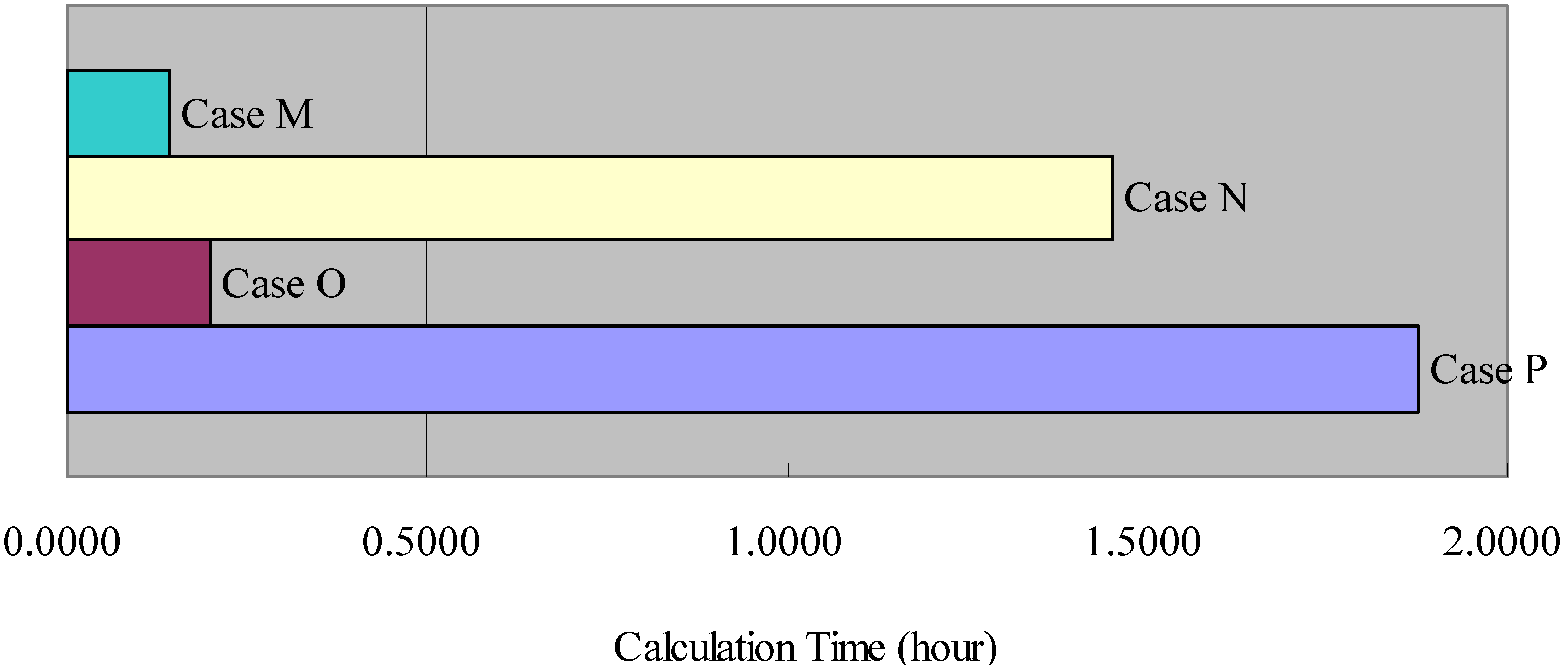
Part 4: The comparison about the processing efficiency.

The processing efficiencies of different methods are compared here. In this simulation, all the uncertainty factors are considered, including the generators, the transmission lines and the loads. Table 11 gives the adopted methods for Case M to Case P, where the number of simulations is set as N = 100. The calculation time for each case is shown in Figure 4.

Table 11. The adopted methods of Case M, Case N, Case O and Case P.

Case	Bootstrap Method	Dual-core Parallel Computing Technique
M	√	√
N	×	√
O	√	×
P	×	×

“√” means the method is adopted and “×” means the method is not adopted. If the bootstrap method is used, set M = 80, W = 10; otherwise set M = 800, W = 0.

Table 11. The adopted methods of Case M, Case N, Case O and Case P.

Case	Bootstrap Method	Dual-core Parallel Computing Technique
M	√	√
N	×	√
O	√	×
P	×	×

“√” means the method is adopted and “×” means the method is not adopted. If the bootstrap method is used, set M = 80, W = 10; otherwise set M = 800, W = 0.

Figure 4. The comparison of calculation times.

Figure 4. The comparison of calculation times.

From Figure 4, the calculation time of Case M is only about one tenth that of Case N, and about seven tenths that of Case O. Therefore, the bootstrap method can greatly improve the processing speed, while the multi-core parallel computing technique can reduce the calculation time to some extent. Despite the help of the bootstrap method and the multi-core parallel computing technique, due to the restrictions of the calculation platform, the calculation time of the proposed method is still considerable. This is due to the time-consuming optimal power flow. Therefore to improve the optimal power flow and further optimize the efficiency of the multi-core parallel computing will be an important future task.

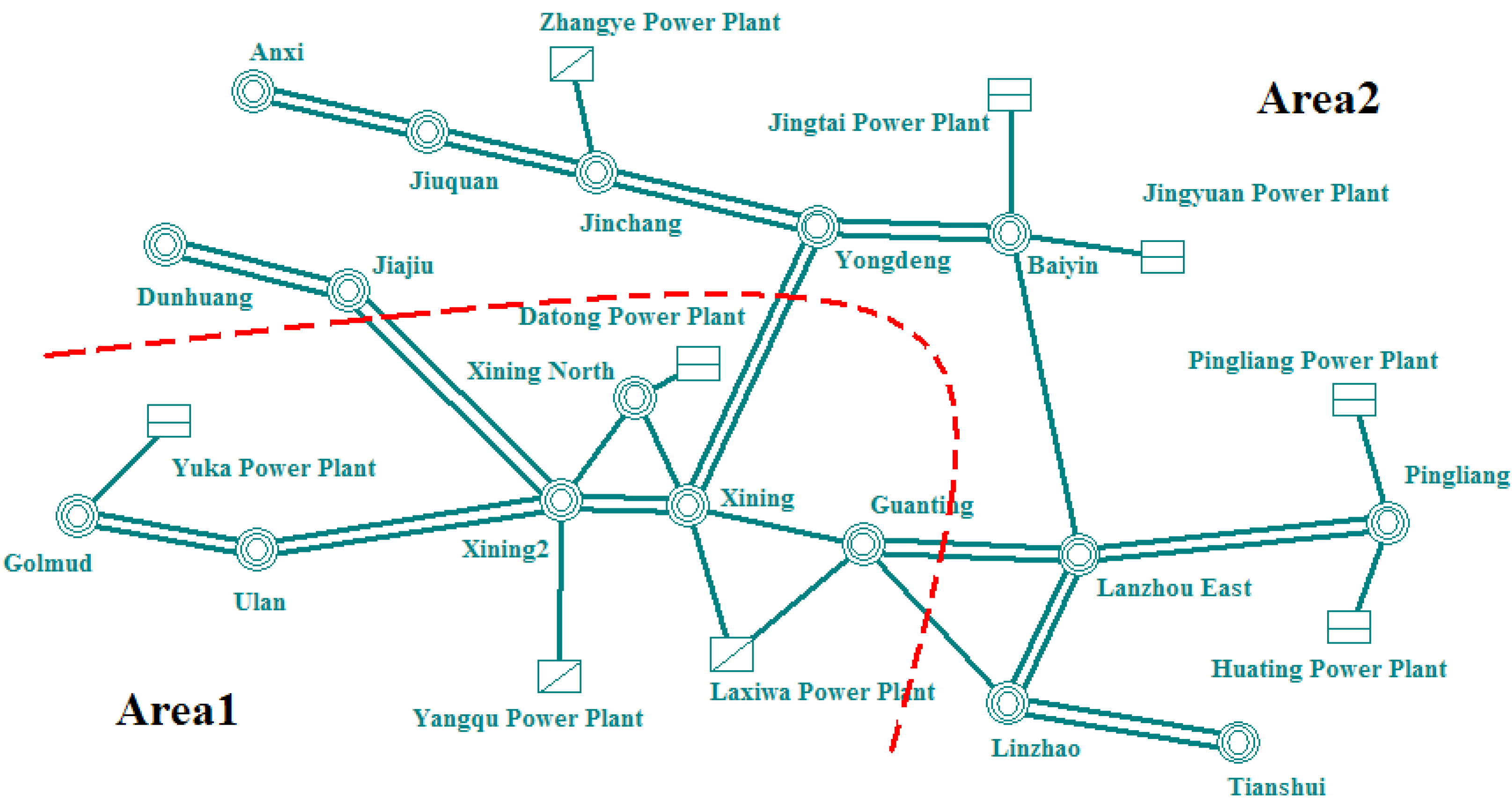
4.2. An Actual Power System in Northwest China

The proposed ATC assessment approach is next applied in an actual power system of two regions in Northwest China. This is a 750 kV planning network for 2020 (the base capacity is 1000 MVA), whose single line diagram is shown in Figure 5. The total active power generation and load are 18,079 MW and 9857 MW, respectively. This paper focuses on the ATC assessment from Area 1 to Area 2. Case Q and Case R are studied. In Case Q a Monte Carlo random simulation (10,000 times) is applied. The proposed approach is used in Case R, and all the uncertainty factors are considered, including the generators, the transmission lines and the loads. The parameters of Case Q and Case R are shown in Table 12, which are based on the historical data in the two regions and the experience of dispatchers. The parameters of random fuzzy simulation are set as follows: N = 3000, M = 80, W = 10.

Figure 5. 750 kV planning network of two regions in Northwest China.

Figure 5. 750 kV planning network of two regions in Northwest China.

The corresponding assessment results are listed in Table 13. When both randomness and fuzziness of generators, transmission lines and loads are considered, the system uncertainty grows significantly. In Case Q and Case R, the variance index increases by about 11%, and the expected value of ATC is reduced by 272 MW, or about 6%. The results calculated using the proposed approach are consistent with current empirical judgments of Transmission Network Operators (TNOs), which for China TNOs, is that the maximum ATC does not exceed 4200 MW. The reduction value is large for the network, and if the fuzziness is not taken into consideration together with randomness, the system maybe becomes unstable in the peak period. Therefore the proposed ATC assessment approach can more comprehensively consider assessment risk, and supply accurate information.

Table 12. The parameters of generators, transmission lines and loads for Case Q and Case R.

Method	Case	Generators		Transmission Lines	Loads
		λG	ξG	ξB	ξL
Monte Carlo random simulation (10,000 times)	Q	0.01	1	0.02	0.02
Random fuzzy simulation	R	0.01	(0.9400, 1, 1.1400)	(0.0100, 0.0190, 0.0400)	(0.0100, 0.0190, 0.0400)

Table 12. The parameters of generators, transmission lines and loads for Case Q and Case R.

Method	Case	Generators		Transmission Lines	Loads
		λG	ξG	ξB	ξL
Monte Carlo random simulation (10,000 times)	Q	0.01	1	0.02	0.02
Random fuzzy simulation	R	0.01	(0.9400, 1, 1.1400)	(0.0100, 0.0190, 0.0400)	(0.0100, 0.0190, 0.0400)

Table 13. The results of Case Q and Case R.

Case	Epro-fuzz,ATC (MW)	Vpro-fuzz,ATC (MW2)
Q	4417	4,702,842
R	4145	5,241,506
Error (%)	−6.1591	11.4540

Table 13. The results of Case Q and Case R.

Case	Epro-fuzz,ATC (MW)	Vpro-fuzz,ATC (MW2)
Q	4417	4,702,842
R	4145	5,241,506
Error (%)	−6.1591	11.4540

5. Conclusions

To consider the two-fold uncertainties in the ATC assessment, this paper proposes a novel ATC assessment approach based on credibility theory, whereby according to the features of both randomness and fuzziness, the corresponding credibility models of generators, transmission lines and loads are comprehensively built up for the first time; then the random fuzzy simulation is applied in the ATC assessment; the bootstrap method and the multi-core parallel computing technique are adopted to enhance the computation speed. By testing on the IEEE-30 bus system and an actual system in China, the viability of the proposed models and algorithm is verified. Preliminary research is done on the sensitivity analysis to the fuzzy influencing factors of ATC and as a result, it gives a way to reduce the fluctuation of ATC.

Randomness and fuzziness are two general features in power systems. Compared with the traditional Monte Carlo random simulation, which only considers the randomness, the proposed method can coherently consider both uncertainties. Random variables that can perhaps adopt different values with certain probabilities can get the same results of the ATC assessment, but this modeling is not sensible. For example, for a generator it means to improve its forced outage rate. However, when the generator is in an on-state, its available output is greatly affected by many external factors, and not a fixed value, so it cannot be described by improving the forced outage rate, and a random variable is not appropriate, while our proposed random fuzzy variable can more suitably describe both the random forced outage rate and the fuzzy available output of a generator at the same time. The proposed method can effectively reduce the assessment risk, and supply accurate information for the mid- and long-term planning of power systems. This will have a better potential of development and application in power source and grid planning and operation. However, the proposed method can only be used with detailed parameters which refer to both randomness and fuzziness. For multiple area power systems, different TSOs share limited information. Therefore to deal with this case, we have carried out some exploratory research on building clustering models of generators, transmission lines and loads, using a multi-agent approach. This will be reported in future publications.

References

1. North American Electric Reliability Council (NERC). Available Transfer Capability Definitions and Determination; NERC: Swindon, UK, 1996. [Google Scholar]
2. Power Systems Engineering Research Center (PSERC). Electric Power Transfer Capability: Concepts, Applications, Sensitivity and Uncertainty; PSERC Publication: Tempe, AZ, USA, 2001. [Google Scholar]
3. Sauer, P.W. Alternatives for calculating transmission reliability margin (TRM) in available transfer capability. In Proceedings of the Thirty-First Hawaii International Conference, Kona, HI, USA, 6–9 January 1998; p. 89.
4. Ou, Y.; Singh, C. Assessment of Available Transfer Capability and Margins. IEEE Trans. Power Syst. 2002, 17, 463–468. [Google Scholar]
5. Shin, D.-J.; Kim, J.-O.; Kim, K.-H.; Singh, C. Probabilistic approach to available transfer capability calculation. Electr. Power Syst. Res. 2007, 77, 813–820. [Google Scholar] [CrossRef]
6. Akbari, T.; Rahimikian, A.; Kazemi, A. A multi-stage stochastic transmission expansion planning method. Energy Convers. Manag. 2011, 52, 2844–2853. [Google Scholar] [CrossRef]
7. Liu, B.; Liu, Y.-K. Expected value of fuzzy variable and fuzzy expected value models. IEEE Trans. Fuzzy Syst. 2002, 10, 445–450. [Google Scholar]
8. Liu, B. Toward fuzzy optimization without mathematical ambiguity. Fuzzy Optim. Decis. Mak. 2002, 1, 43–63. [Google Scholar] [CrossRef]
9. Liu, B. Uncertainty Theory: An Introduction to Its Axiomatic Foundations; Springer-Verlag: Berlin/Heidelberg, Germany, 2004. [Google Scholar]
10. Liu, B. A survey of credibility theory. Fuzzy Optim. Decis. Mak. 2006, 5, 387–408. [Google Scholar] [CrossRef]
11. Liu, B.; Liu, Y.-K. Expected value operatot of random fuzzy variable and random fuzzy expected value models. Int. J. Uncertain. Fuzziness Knowl.-Based Syst. 2003, 11, 195–215. [Google Scholar] [CrossRef]
12. Feng, Y.; Wu, W.; Zhang, B.; Li, W. Power system operation risk assessment using credibility theory. IEEE Trans. Power Syst. 2008, 23, 1309–1318. [Google Scholar] [CrossRef]
13. Feng, Y.; Wu, W.; Zhang, B.; Sun, H.; Wang, S. Hydro-thermal generator maintenance scheduling based on credibility theory. Proc. Chin. Soc. Electr. Eng. 2006, 26, 14–19. [Google Scholar]
14. Ma, X.; Liu, J.; Wen, F. Random-fuzzy programming model for developing optimal bidding strategies in the uncertain environment. Proc. Chin. Soc. Electr. Eng. 2009, 29, 77–83. [Google Scholar]
15. Wu, J.; Wu, Q.; Chen, G.; Liang, Y.; Zhou, J. Fuzzy random chance-constrained programming for quantifying the transmission reliability margin. Autom. Electr. Power Syst. 2007, 31, 23–28. [Google Scholar]
16. Kwakernaak, H. Fuzzy random variables I. Inf. Sci. 1978, 15, 1–29. [Google Scholar] [CrossRef]
17. Kwakernaak, H. Fuzzy random variables II. Inf. Sci. 1979, 17, 253–278. [Google Scholar] [CrossRef]
18. Zhou, J.; Liu, B. Analysis and algorithms of bifuzzy systems. Int. J. Uncertain. Fuzziness Knowl.-Based Syst. 2004, 12, 357–376. [Google Scholar] [CrossRef]
19. Liang, R.-H.; Liao, J.-H. A fuzzy optimization approach for generation scheduling with wind and solar energy systems. IEEE Trans. Power Syst. 2007, 22, 1665–1674. [Google Scholar] [CrossRef]
20. Kaufmann, A. Introduction to the Theory of Fuzzy Subsets; Academic Press: Waltham, MA, USA, 1975. [Google Scholar]
21. Zadeh, L.A. Fuzzy sets as a basis for a theory of possibility. Fuzzy Sets Syst. 1978, 1, 3–28. [Google Scholar] [CrossRef]
22. IEEE Power & Energy Society. IEEE Standard Definitions for Use in Reporting Electric Generating Unit Reliability, Availability, and Productivity; ANSI/IEEE Std 762-1987; IEEE Power & Energy Society: Piscataway, MJ, USA, 1998. [Google Scholar]
23. Feng, Y.; Wu, W.; Zhang, B.; Sun, H.; He, Y. Short-term transmission line maintenance scheduling based on credibility theory. Proc. Chin. Soc. Electr. Eng. 2007, 27, 65–71. [Google Scholar]
24. Ding, M.; Dai, R.; Hong, M.; Xu, X. Simulation to the weather condition affecting the reliability of transmission network. Autom. Electr. Power Syst. 1997, 21, 18–20. [Google Scholar]
25. Duman, S.; Güvenç, U.; Sönmez, Y.; Yörükeren, N. Optimal power flow using gravitational search algorithm. Energy Convers. Manag. 2012, 59, 86–95. [Google Scholar] [CrossRef]
26. Mahdada, B.; Bouktir, T.; Srairi, K.; EL Benbouzidc, M. Dynamic strategy based fast decomposed GA coordinated with FACTS devices to enhance the optimal power flow. Energy Convers. Manag. 2010, 51, 1370–1380. [Google Scholar] [CrossRef] [Green Version]
27. Efron, B.; Tibshirani, R.J. An Introduction to the Bootstrap; Chapman and Hall/CRC Press: London, UK; Boca Raton, FL, USA, 1993. [Google Scholar]
28. Khosravi, A.; Nahavandi, S.; Creighton, D. A neural network-GARCH-based method for construction of prediction intervals. Electr. Power Syst. Res. 2012, 96, 185–193. [Google Scholar] [CrossRef]
29. Zimmerman, R.D.; Murillo-Sánchez, C.E.; Thomas, R.J. MATPOWER’s extensible optimal power flow architecture. In Proceedings of the Power and Energy Society General Meeting, Calgary, AB, Canada, 26–30 July 2009; pp. 1–7.
30. Shaaban, M.; Liu, H.; Li, W.; Yan, Z.; Ni, Y.; Wu, F. ATC calculation with static security constraints using benders decomposition. Proc. Chin. Soc. Electr. Eng. 2003, 23, 7–11. [Google Scholar]