Article

Effects of Surface Wettability and Roughness on the Heat Transfer Performance of Fluid Flowing through Microchannels

Airport School, Civil Aviation University of China, Tianjin 300300, China
*
Author to whom correspondence should be addressed.
These authors contributed equally to this work.
Energies 2015, 8(6), 5704-5724; https://doi.org/10.3390/en8065704
Submission received: 31 January 2015 / Accepted: 9 June 2015 / Published: 16 June 2015

Abstract

:
The surface characteristics, such as wettability and roughness, play an important role in heat transfer performance in the field of microfluidic flow. In this paper, the process of a hot liquid flowing through a microchannel with cold walls, which possesses different surface wettabilities and microstructures, is simulated by a transient double-distribution function (DDF) two-phase thermal lattice Boltzmann BGK (LBGK) model. The Shan-Chen multiphase LBGK model is used to describe the flow field and the independent distribution function is introduced to solve the temperature field. The simulation results show that the roughness of the channel wall improves the heat transfer, no matter what the surface wettability is. These simulations reveal that the heat exchange characteristics are directly related to the flow behavior. For the smooth-superhydrophobic-surface flow, a gas film forms that acts as an insulating layer since the thermal conductivity of the gas is relatively small in comparison to that of a liquid. In case of the rough-superhydrophobic-surface flow, the vortex motion of the gas within the grooves significantly enhances the heat exchange between the fluid and wall.

1. Introduction

Microfluidics has become particularly active during the last few years since it has been widely used in many fields, thus, an understanding of fluid flow on the micro scale is crucial. Previous studies have indicated that the surface wettability has a significant impact on the fluid flow behavior and heat transfer performance. Moreover, numerous experiments have shown that rough surfaces with microstructures can directly increase surface hydrophobic properties. The surfaces which are covered with micrometer scale pots are strongly repellent to water, which rapidly increases the contact angle up to 160°. This should be compared to the more traditional ways of increasing the contact angle, such as surface coatings and chemical modifications, whereby it is difficult to achieve an angle of more than 120°. Therefore, either the effect of surface wettability or the effect of surface roughness is extremely important for the micro-fluid flow.
Previous studies mainly focused on the flow behaviors. Zhang [1] investigated the contact line and contact angle dynamic of fluid flowing in superhydrophobic channels. Jeffs [2] predicted the turbulent channel flow with superhydrophobic walls consisting of micro-ribs and cavities oriented parallel to the flow direction. Chibbaro [3] studied the effect of geometrical obstacles in microchannels on the process of capillary filling. Lauga [4] and Ybert [5] analyzed the slip velocity in channels by computational fluid dynamics (CFD) methods. Davies [6] and Ou [7] analyzed the drag reduction performance of fluid flowing through microchannels with different wettability and roughness walls. Our previous work [8] investigated the flow behaviors and the effects of surface wettability and roughness in details by a lattice Boltzmann method. Additionally, there are also abundant theoretical research [9,10] on the flow upon the rough superhydrophobic surface, and the relationship between surface roughness and its wettability had been analyzed [11,12] as well. However, reports on the heat exchange performance using a superhydrophobic surface are rare. Whether the heat exchange rate could be enhanced or not is still an unsettled issue and the heat transfer mechanism is still not clarified. Therefore, the aim of this paper was to examine the heat exchange abilities of fluid flowing over rough superhydrophobic surfaces. The effects of wettabilities and roughness on heat transfer performance will be investigated by a numerical approach.
The macroscopic flow and heat exchange are closely related to the microscopic structure, which makes the problem become so complex that research is not an easy task. Fortunately, the lattice Boltzmann method (LBM), as an alternative numerical approach on mescoscopic level between the traditional macroscopic CFD and the microscopic molecular dynamics (MD) methods, is quite appropriate to describe microscale flow and the involved heat transfer problems, because the arithmetic itself is developed based on the microscale flow mechanism. Instead of solving the usual continuum hydrodynamic equations of the conserved field, the LB approach describes the fluid flow by tracking the evolution of the distribution function of microscopic fluid particles, which makes the LB method possess some important features that distinguish it from other numerical methods. In recent years, the LB model has achieved great success in simulations of microscopic fluid flows.
In this paper, the lattice Boltzmann method is used to investigate flow behavior and heat exchange performance when a hot liquid flows through cold channels with different wettabilities and topographical surfaces. The paper is organized as follows: the LBM algorithm is formulated in Section 2; the validation of the code by the benchmark solution presented in Section 3; the numerical simulation results are presented in Section 4; and finally, the conclusions are drawn in Section 5.

2. Lattice Boltzmann Method

In this study, the process of a hot liquid flowing into a cold microchannel with different surface wettabilities and roughnesses is investigated by the LB method. Originally, only mass and momentum conservations were considered in the LB model, however, in many applications it is important and sometimes critical to consider the temperature distribution in the fluid flows. The thermal LB methods have received wide attention and several models have been developed. However, most emphasis has been laid on single-phase flows while thermal models for multiphase flow are lacking. Therefore, in this research, the multiphase thermal LBM is developed to predict the temperature distribution of a multiphase flow.
For the single-phase flow, the existing thermal models can be classified into two categories: the multispeed (MS) approach [13,14] and the multi-distribution function (MDF) approach [15]. The MS approach is a straightforward extension of the isothermal LB model in which the energy conservation is implemented by adding additional speeds and by including the higher-velocity terms in the equilibrium distribution. Although theoretically possible, the MS approach suffers from numerical instability and a narrow range of temperature variation. Most of all, the most obvious restriction is the impossibility of varying the Prandtl number. In the MDF approach, the temperature field is also solved using an LB equation by introduction of an independent distribution function. The thermal diffusivity is independent of the viscosity, which results in a changeable Prandtl number in simulations. The MDF model can improve the numerical stability and the range of temperature variations. The accuracy of the MDF models has been verified by several benchmark studies [16,17]. Thus, in our research, the double-distribution function (DDF) multiphase LB model is used, where the D2Q9 Shan-Chen multiphase LB equation is used to describe the flow field, while the D2Q5 thermal LB equation is adopted to simulate the temperature field.

2.1. LB Flow Field Equations

Initially, the cold channel is filled with a cold gas, and then the hot liquid flows into the channel and displaces the gas. The process should be described by the two-phase model. There are several models available for modeling multiphase fluid flows, including the chromodynamics model [18], Shan-Chen model [16] (also known as pseudo-potential), free energy model [19,20] and others [21,22,23]. In the present study, the Shan-Chen model is chosen to solve the velocity field because of its ability to handle fluids with different densities, to separate the interface automatically, and to easily implement the different wettability conditions.
In the LB model the fluid is described by quantities fi representing the particle density distribution (PDF) in the ith velocity direction of the lattice:
f i = f i ( x , t )       i = 0 , 1 , M
where x is the position on the lattice and t is the time. M represents the number of velocity directions of the particle at each node of the lattice.
The established LBGK model [24] in which the collision operator is simply approximated by a linear expression proposed by Bhatnagar, Gross, and Krook (BGK) [25] is widely used due to its simplicity. Then the equation of fi is:
f i ( x + e i δ t , t + δ t ) = f i ( x , t ) 1 τ υ [ f i ( x , t ) f i ( e q ) ( x , t ) ]
In this relation, the relaxation parameter τ υ expresses the rate at which the local particle distribution f i ( x , t ) relaxes to the local equilibrium state f i ( e q ) ( x , t ) . For the velocity field, a two-dimensional regular grid with a nine-velocity lattice (the so-called D2Q9 topology), as shown in Figure 1a, is considered and the velocities e i are given by:
e i = { ( 0 , 0 ) ( cos ( i 1 ) π / 2 ) , sin ( i 1 ) π / 2 ) ) 2 ( cos ( 2 ( i 5 ) + 1 ) π / 4 ) , sin ( 2 ( i 5 ) + 1 ) π / 4 ) )      i = 0 i = 1 , 2 , 3 , 4 i = 5 , 6 , 7 , 8
Figure 1. Lattice geometry and velocity vectors of (a) the D2Q9 model and (b) the D2Q5model.
Energies 08 05704 g001
In this case, f i ( e q ) , the corresponding equilibrium distribution function (EDF) can be expressed as:
f i ( e q ) = w i ρ [ 1 + e i u e q c s 2 + ( e i u e q ) 2 2 c s 4 u e q u e q 2 c s 2 ]
with the weights w 0 = 4 / 9 , w i = 1 / 9 for i = 1 , 2 , 3 , 4 and w i = 1 / 36 for i = 5 , 6 , 7 , 8 and c s = c / 3 is defined as the lattice speed of sound for the D2Q9 lattice. Here c = δ x / δ t is the lattice speed, and for simplification purposes, c is set as unity under the assumption that the lattice spacing δ x and the time step δ t are unity as well.
At each lattice, all the forces will be incorporated into Equation (4) by shifting the equilibrium velocity u e q :
u e q ( x , t ) = u ( x , t ) + τ υ   F ( x , t ) / ρ ( x , t )
where F ( x , t ) = F σ ( x , t ) + F t ( x , t ) is the total force acting on the fluid, including the fluid/fluid interaction F σ and the fluid/solid interaction F t . The flow investigated in the present work is on a horizontal surface, the effect of gravity therefore is not taken into account. The fluid/fluid interaction F σ ( x ) can be expressed in the following form:
F σ ( x ) = ψ ( x ) x G ( x , x ) ψ ( x ) ( x x )
where the Green function G ( x , x ) is a constant, given as G ( x , x ) = G for e i = c , G ( x , x ) = G / 4 for e i = 2 c and G ( x , x ) = 0 for other cases. The value of G controls the strength of the interacting force between different phases. By varying G, different surface tensions can be obtained. ψ is the interaction potential, according to Shan and Chen’s research, it must be monotonically increased and bounded. The extensively used scheme ψ ( ρ ) = ρ [ 1 exp ( ρ / ρ ) ] [26,27] is employed in this model.
Similarly, the interaction between the fluid and the solid surface F t ( x ) , which is determined by the presence of a solid in the nearest and the next nearest neighbours that surrounding a fluid node, has the form:
F t ( x ) = G t ψ ( x ) i s ( x + e i ) ( x x )
where s is an indicator function of a solid phase, s = 1 or s = 0 is for fluid or solid, respectively. By adjusting G t , surface wetting characteristics can be controlled.
Physical quantities of fluid flow, such as density ρ and velocity u, can be obtained through moment summations in the velocity space:
ρ ( x , t ) = i = 0 M f i ( x , t )
u ( x , t ) = i = 0 M f i ( x , t ) e i / ρ ( x , t )
The continuity and Navier–Stokes equations through a Chapman–Enskog expansion [24,28,29] can be recovered. Accordingly, the kinematic viscosity (in lattice units) is defined by:
υ = c s 2 δ t ( τ υ 0.5 )
and the equation of state (EOS) is given by:
p = c s 2 ρ + c 0 2 G 2 ψ 2 ( ρ )
where c0 is the constant depending on the lattice structure, for the D2Q9 lattices, c 0 = 6 .

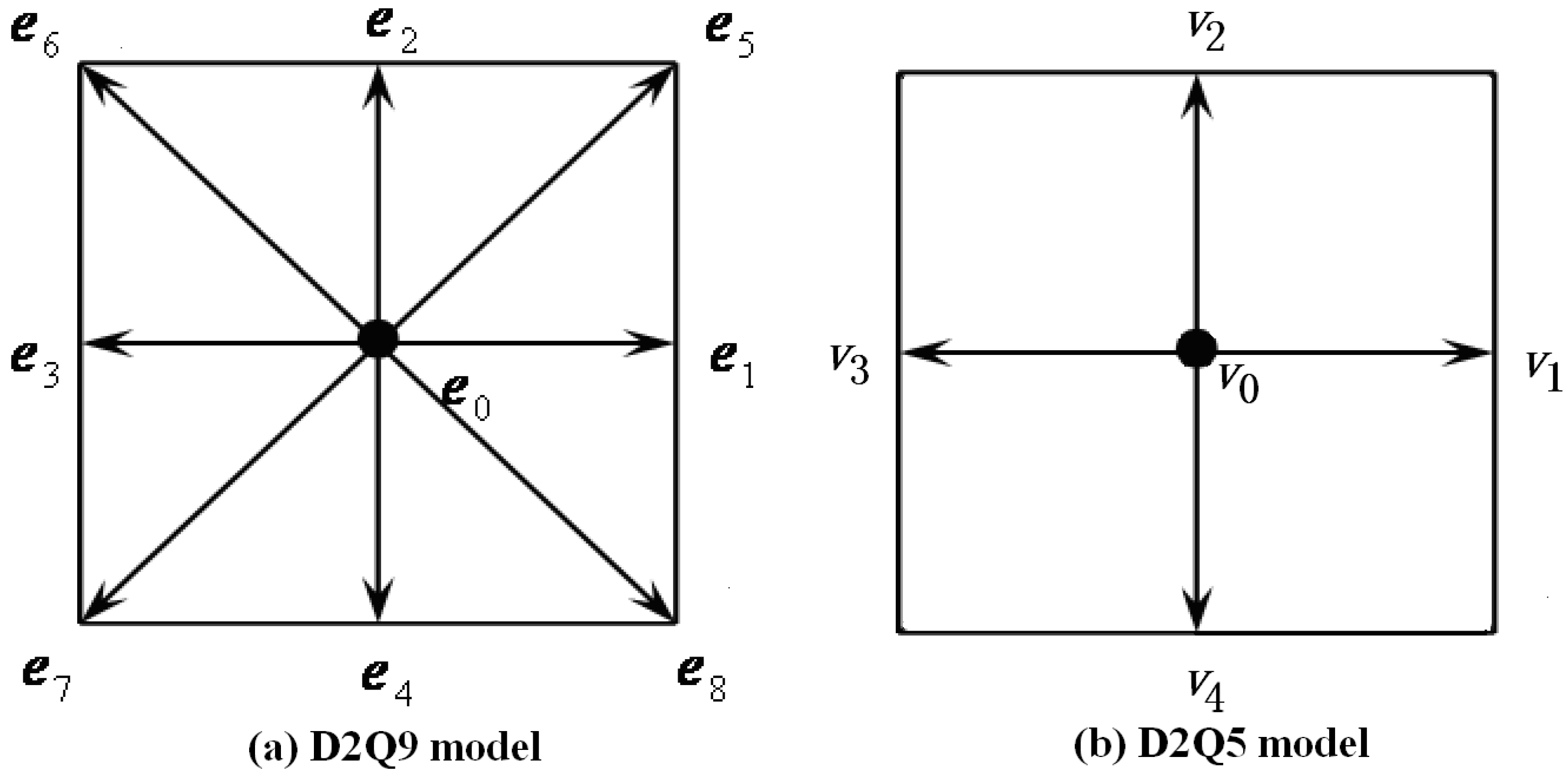
2.2. LB Equations for Temperature Field

An independent distribution function is introduced to solve the temperature field and given as follows:
g i ( x + v i δ t , t + δ t ) = g i ( x , t ) 1 τ T [ g i ( x , t ) g i ( e q ) ( x , t ) ]
The LBGK model for PDFs in the temperature field is similar to that in velocity field, but a simplified EDF can be used:
g i ( e q ) = w i T T [ 1 + v i u e q c s T 2 ]
For a D2Q5 topology, as shown in Figure 1b, the lattice velocities for temperature field, v i , are:
v i = { ( 0 , 0 ) ( cos ( ( i 1 ) π / 2 ) , sin ( ( i 1 ) π / 2 )      i = 0 i = 1 , 2 , 3 , 4
The associated weights w i T are w 0 T = 1 / 3 and w i T = 1 / 6 for i = 1 , 2 , 3 , 4 . For the D2Q5 model, c s T = c / 2 is the lattice speed of the sound in the temperature field. At each lattice node, the temperature is defined as:
T ( x , t ) = i = 0 4 g i ( x , t )
The Chapman–Enskog expansion for the temperature distribution function recovers the macroscopic energy equation. This gives the thermal diffusivity, κ, in term of the single relaxation:
κ = c s T 2 δ t ( τ T 0.5 )

2.3. Variable Relaxation Times Treatment
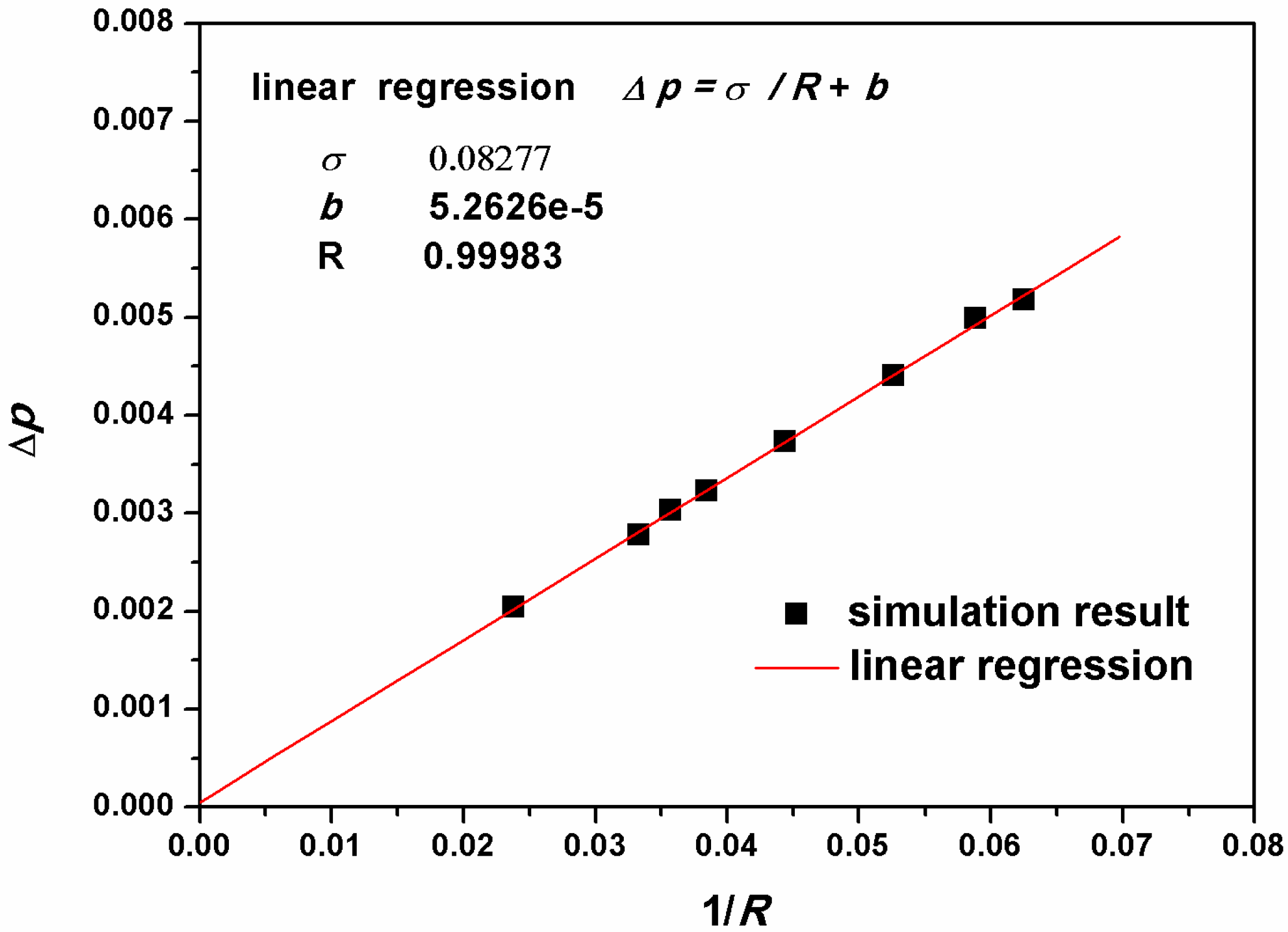
In the present model the properties, including density, velocity and thermal diffusivity, are different for the two phases. Density ratio ς, viscosity ratio ξ and thermal diffusivity ratio γ are defined as the ratios of the liquid phase properties to the gas phase properties ( ς = ρ l / ρ g , ξ = υ l / υ g and γ = κ l / κ g ). For each grid, the liquid phase fraction α l is introduced to distinguish the different phases expressed as:
α l = { 0    ρ ρ g ρ ρ g ρ l ρ g    ρ g < ρ < ρ l 1    ρ ρ l
Thus, the average viscosity and thermal diffusivity can be calculated as below:
υ = ( 1 α l ) υ g + α l υ l
κ = ( 1 α l ) κ g + α l κ l
Accordingly, the dimensionless relaxation times, for both flow field and temperature field, are also variable. They can be determined by Equation (10) and Equation (16). The accuracy and stability of numerical simulation can be guaranteed by adjusting the time step δ t and the lattice speed c, and the details can be found in [30], where it is suggested that the relaxation times should fall into the range between 0.5 to 2.

3. Benchmark Tests

Two benchmark tests are conducted to validate the reliability of the proposed LB model: (a) the Laplace law should be satisfied and (b) the temperature-drop curve obtained by LBM agrees well that simulated by the classical CFD model.
Primarily, spheroidal droplets with different radii are generated in the center of a 150 × 150 lattice domain in an isothermal system. No any external forces, such as gravity, are introduced. A periodic boundary condition is imposed on each boundary of the domain. We set ς = 10 , ξ = 10 and G = 0.6 for all simulations. The droplets evolve towards a steady state. Their radii and inside/outside pressures ( Δ p = p i n p o u t ) under the steady state are measured. The relationship between Δ P and 1 / R is presented in Figure 2. The slope of a plot of 1 / R vs. Δ p will be the surface tension in accordance with the Laplace law which gives the relationship between the final radii of the droplet and pressure difference as Δ p = σ / R . The LBM result agrees well the Laplace law. In the case of G = 0.6 , the surface tension σ is 0.08277 (in lattice units) and the intercept at y-axis is can be considered as zero ( b = 5.2626 e 5 ). It can be seen that LBM results agree well with the Laplace law when G = 0.6 . Therefore, this result will be adopted in the following studies.
Figure 2. Relationship between 1/R and Δ p in the case of G = 0.6 .
Energies 08 05704 g002
Next the heat transfer will be taken into account. Initially, a hot liquid droplet ( T l , i n i = 1 ) with the radius of 25 lattices, which is surrounded by gas at low temperature ( T g , i n i = 0 ), is put in the center of the computational domain (150 × 150 lattice system). The Prandtl number ( Pr l = ν l / κ l ) is set to be 1 and the other required parameters are set as follows: ς = 10 , ξ = 10 , G = 0.6 . The diffusivity ratio γ varies from 1 to 10. All boundaries are set as solid walls with constant low temperature and the bounce-back boundary condition is employed for the flow field. The heat transfer will take place between the liquid droplet and the surrounding gas. The average temperature of liquid droplet with the time elapsing is presented in Figure 3. The dimensionless temperature and time in this figure are defined as T = T l , a / ( T l , i n i T g , i n i ) and t = κ l t / R 2 , respectively.
Figure 3. Comparisons of the average temperatures of liquid droplet between the LB method and the level set approach. (The horizontal coordinate is dimensionless temperature T = T l , a / ( T l , i n i T g , i n i ) and the ordinate coordinate is dimensionless time t = κ l t / R 2 ).
Energies 08 05704 g003
For the sake of validation, this problem is simulated by the traditional CFD method, which is derived from the continuum-based steady-stage conservation equations of mass, momentum and energy. There are two phases, gas and liquid, coexisting in the computational domain, thus, the VOF method, a surface-tracking technique applied to a fixed Eulerian mesh, is used to track the volume fraction of each phase. In order to track the gas-liquid interface, one continuity equation are solved for each phase. For liquid phase, this equation has the following form:
1 ρ l [ ( t ( α l ρ l ) + ( α l ρ l u l ) ] = 0
A single momentum equation is solved throughout the domain, and the resulting velocity field is shared among the phases. The momentum equation, shown below, is dependent on the volume fractions of all phases.
t ( ρ u ) + ( ρ u u ) = p + [ μ ( u + u T ) ]
The energy equation, also shared among the phases, is shown below:
t ( ρ E ) + [ u ( ρ E + p ) ] = ( κ T )
The properties appearing in the transport equations, such as density, velocity, pressure, thermal conductivities, viscosity, are determined by the presence of the component phases in each control volume. In the gas-liquid system, the density in each cell is given by ρ = ρ l α l + ρ g ( 1 α l ) . All other properties could be computed in this manner. The values of properties for each phase are set as the same ones used in the LBM simulations. The mass, momentum and temperature governing equations are discretized using the second order upwind scheme. The SIMPLE algorithm is applied for pressure-velocity coupling. The governing equations are solved iteratively until they are convergent and the convergence criterion is 10−6 for all variables. The governing equations are solved on the Fluent 6.3.26® platform, and an 88-node Intel Xeon E5420 Linux cluster is employed to accomplish the solution iteration processes. Figure 3 shows that the LBM results agree very well with the results obtained by the traditional CFD method with a maximum error of less than 5.6%. This proves that the present multiphase thermal LBM is able to predict the flow behaviour and the heat transfer characteristics.

4. Numerical Simulation

In this section, the heat transfer characteristics with different wettability surfaces have been investigated. Two types of channel flows (smooth-surface channel flow and rough-surface channel flow) are simulated.

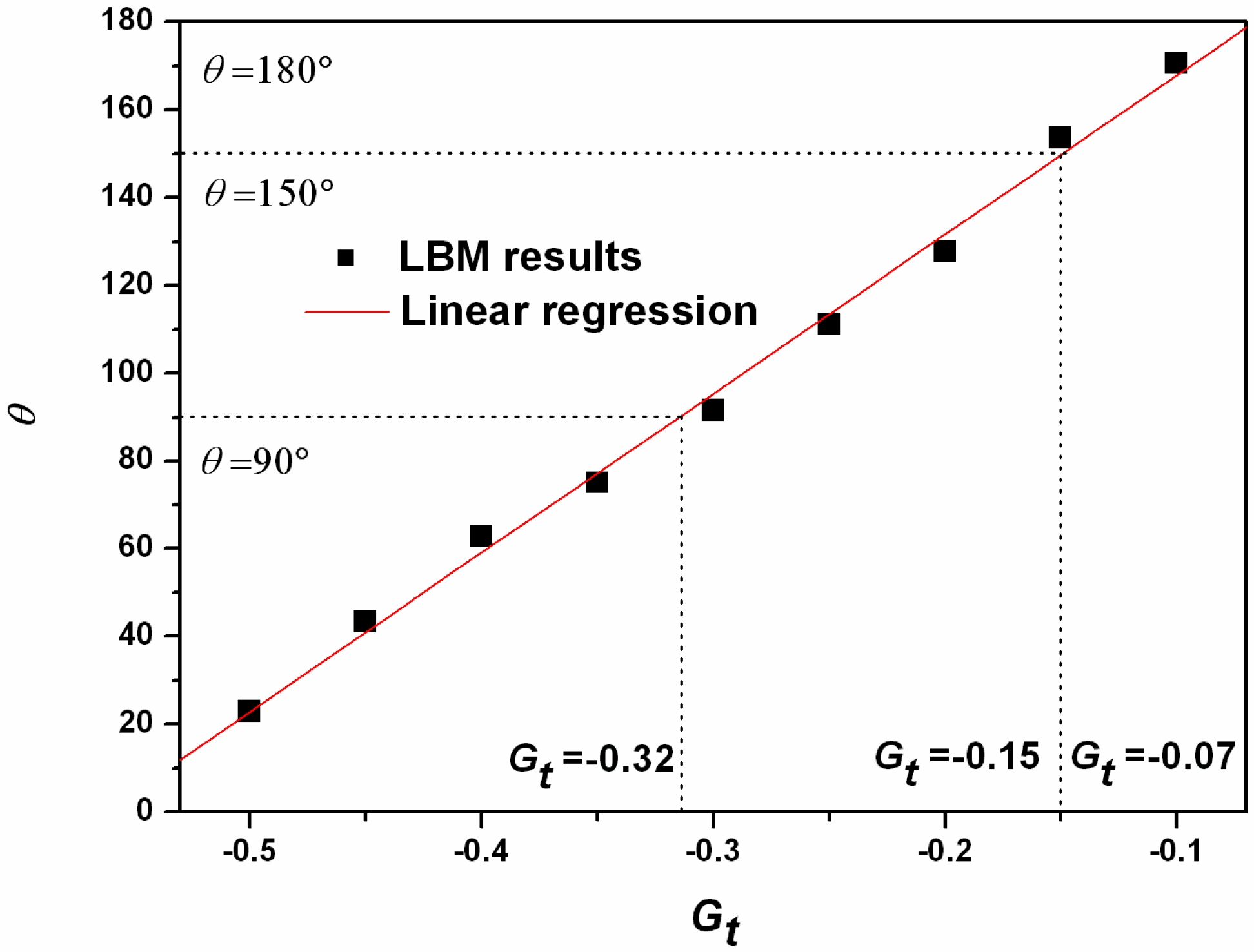
4.1. Different Wettabilities Treatment

In the present model, the different surface wettabilities can be obtained by varying the fluid/solid interaction parameter G t . In order to obtain their relationship, some pre-simulations must be made. In the isothermal system, a spheroidal liquid droplet is placed on the bottom surface. The periodic boundary condition is adopted for both left and right hand sides and the bounce-back boundary condition is employed for both top and bottom to reproduce no-slip boundary conditions. ς = 10 , ξ = 10 , G = 0.6 are used in these cases and the values of G t changes from 0 to −0.4. Due to the fluid/solid interaction, evolution of the droplets will take place and their steady states will clearly not be the same. The droplets spread on the surface with different contact angles. The floating phenomenon is observed when G t = 0.07 , in that case, the contact angle can be considered as 180°. It can be seen from the simulation data that the static contact angle is a linear function of the fluid/solid interaction parameter, where it increases with the increase of G t , as shown in Figure 4.
Figure 4. Relationship between static contact angle θ and fluid/solid interaction parameter G t in the case of G = 0.6 .
Energies 08 05704 g004
Some useful information can be gained: in the case of G t < 0.32 , 0.32 < G t < 0.15 and 0.15 < G t < 0.07 , the corresponding contact angle will be lower than 90°, higher than 90° but lower than 150° and higher than 150°, namely the surface is the hydrophilic, hydrophobic and superhydrophobic, respectively.

4.2. Solution Scheme and Procedure

In our previous research [8], the flow behaviour had been investigated and the results indicated that the flowing resistance can be reduced by using a superhydrophobic surface, so in this paper, the emphasis will be laid upon the heat transfer performance. Channel flow with smooth surfaces as well as rough surfaces are simulated. Rectangular roughness elements distributed at equivalent distances are used to form the rough surfaces at both sides of the channel. The structure scheme of the two types of channels considered are presented in Figure 5.
Figure 5. The structure scheme of channel with smooth surfaces and rough surfaces.
Energies 08 05704 g005
Hot liquid ( T l , i n i = 1 ) flows through the domain with the cold surface ( T w a l l = 0 ) from the inlet side to displace the cold gas (Tg,ini = 0) that initially filled the whole domain. The Poiseuille flow ( u = u max [ 1 ( y n y / 2 ) 2 / ( n y / 2 ) 2 ] , v = 0 ) with Re = 500 is imposed in the inlet side while the outlet side is set as the out-flow condition ( u / x = v / y = 0 ). The top and bottom boundaries are treated as a solid surface with the bounce-back boundary conditions considering the fluid/solid interaction. In this work, ς = 10 , ξ = 10 , γ = 5 and G = 0.6 are used. Five values of G t within the range of −0.4 ~ −0.07 are chosen in this investigation, where the value of −0.4 stands for the hydrophilic surface, values of −0.3, −0.2 for the hydrophobic surface, while value of 0.1 for the superhydrophobic surface. Especially, the ideal hydrophobic surface with a contact angle of 180° ( G t = 0.07 ) is also simulated, although it is still an ideal condition which cannot be found in Nature or manufactured at present. To evaluate the grid size effect on the accuracy of numerical solutions, five sets of lattices are generated to perform the grid-independence tests for channel flow with smooth surfaces and rough surfaces. Table 1 shows the average temperature of the liquid in the case of G t = 0.1 and G = 0.6 at the 200th and 400th steps for different lattices. It can be seen that for the smooth-surface channel flow, the third Grid with the lattice number nx × ny = 200 × 30 gives the approximately the same results as the finest Grid 4 and Grid 5, while for the rough-surface channel flow, the forth Grid with the lattice number nx × ny = 200 × 50 and the roughness elements w = s = 5, h = 10 could obtain similar results as the finest Grid 5. The two set of lattices are adequate to characterize the flow considering both numerical accuracy and computational costs, compared with coarse grid, and thus will be employed for the following calculations in this study.
Table 1. Lattice independence test.
Smooth Channel FlowRough Channel Flow
Lattice numberAverage temperature Lattice numberAverage temperature
nxny200th400th nxnynwnsny200th400th
Grid 1100150.36690.7261Grid 1100252350.30590.6627
Grid 2200150.32920.7058Grid 2150254450.31360.6795
Grid 3200300.38920.7658Grid 31505044100.30290.6573
Grid 4400300.38560.7620Grid 42005055100.32210.6853
Grid 5400600.38010.7592Grid 54001001010200.32020.6823
Simulation conditions: Gt = ‒0.1; G = ‒0.6.

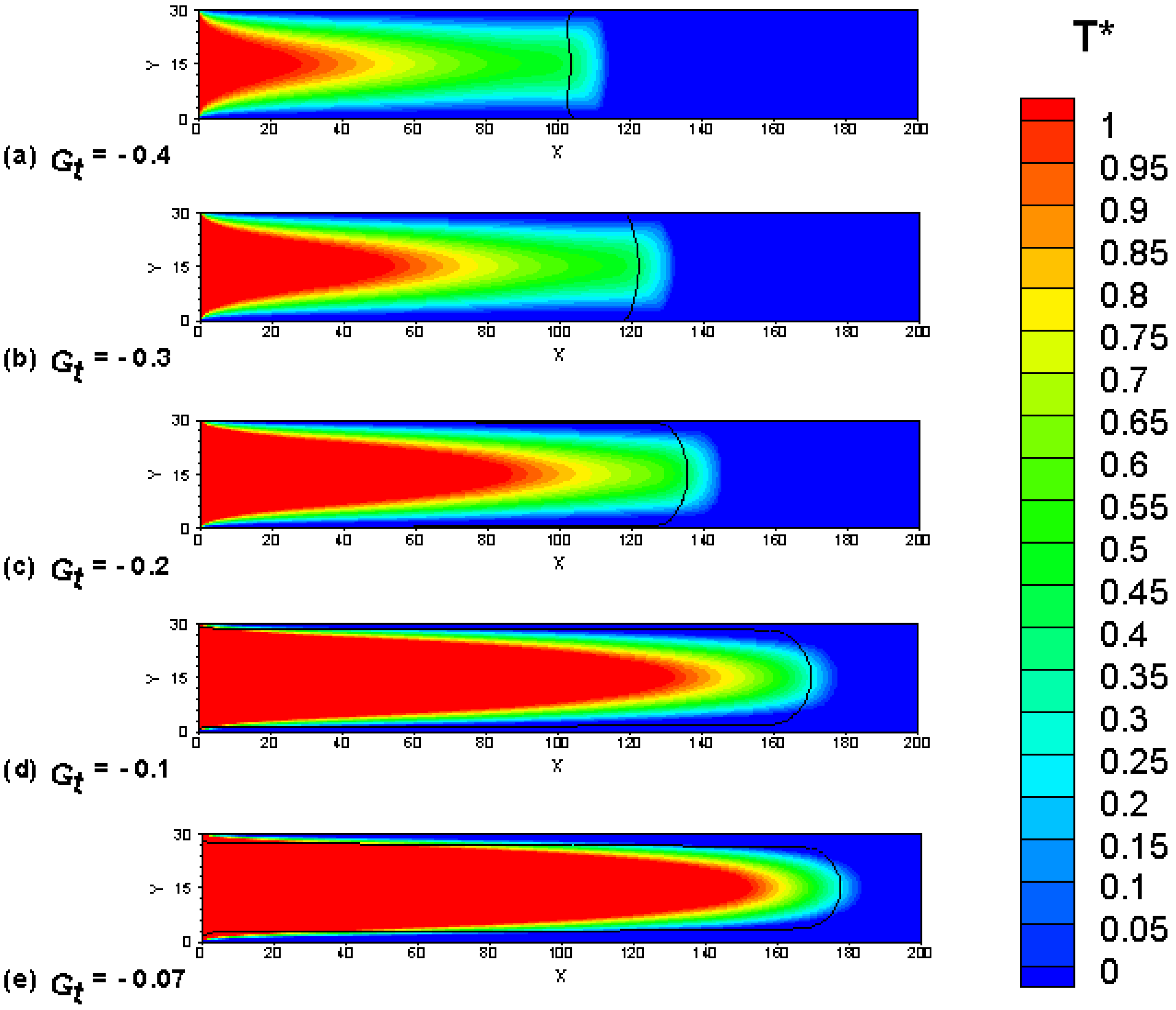
4.3. Simulation Results

The dimensionless temperature distributions at the 400th step are provided in Figure 6, where the black solid line represents the liquid/gas interface. It can be found that the larger the G t is, the longer the liquid flow distance becomes. The explanations on flow length, the flow contact angle and the pressure drop have been presented in our previous works and the details can be found in [8], while the emphasis of this paper is the heat exchange characteristics. During the flow, heat transfer occurs between the liquid/gas interface and between the hot liquid and the cold walls. The hot liquid will be cooled and the heat exchange performance can be considered to be better if the temperature of liquid can be reduced. It can be seen from Figure 6 that the temperature of the liquid apparently becomes higher when G t gets larger, that is to say, the heat transfer performance might be deteriorated when the better-hydrophobic surface is adopted, which seems a disappointing result. Thus, to seek a hydrophobic surface by which not only the pressure drop can be reduced but the heat transfer performance can also be enhanced, the surface roughness must be taken into account.
Then, we take the other study, the heat transfer performance of the channel flow with roughness surface. The roughness elements’ borders are treated as the solid surface with bounce-back boundary conditions with considering the fluid/solid interaction. The other boundaries and parameters are handled by the same approaches as those channel flow cases with smooth surfaces.
The dimensionless temperature distributions of channel flow with rough surface at the 400th step are provided in Figure 7. From the liquid/gas interface (the black solid line), it is obvious that, for the hydrophilic surface ( G t = 0.4 ), liquid sinks into the grooves and fills them, as shown in Figure 7a, and this part of liquid will be cooled by the roughness bumps with constant low temperature. With the increase of G t , the depth that the liquid penetrates into the grooves among the roughness bumps becomes lesser, as shown in Figure 7b–e. However, the cooling performance for the hot liquid gets better. The quantitative analysis will be presented in the next section.

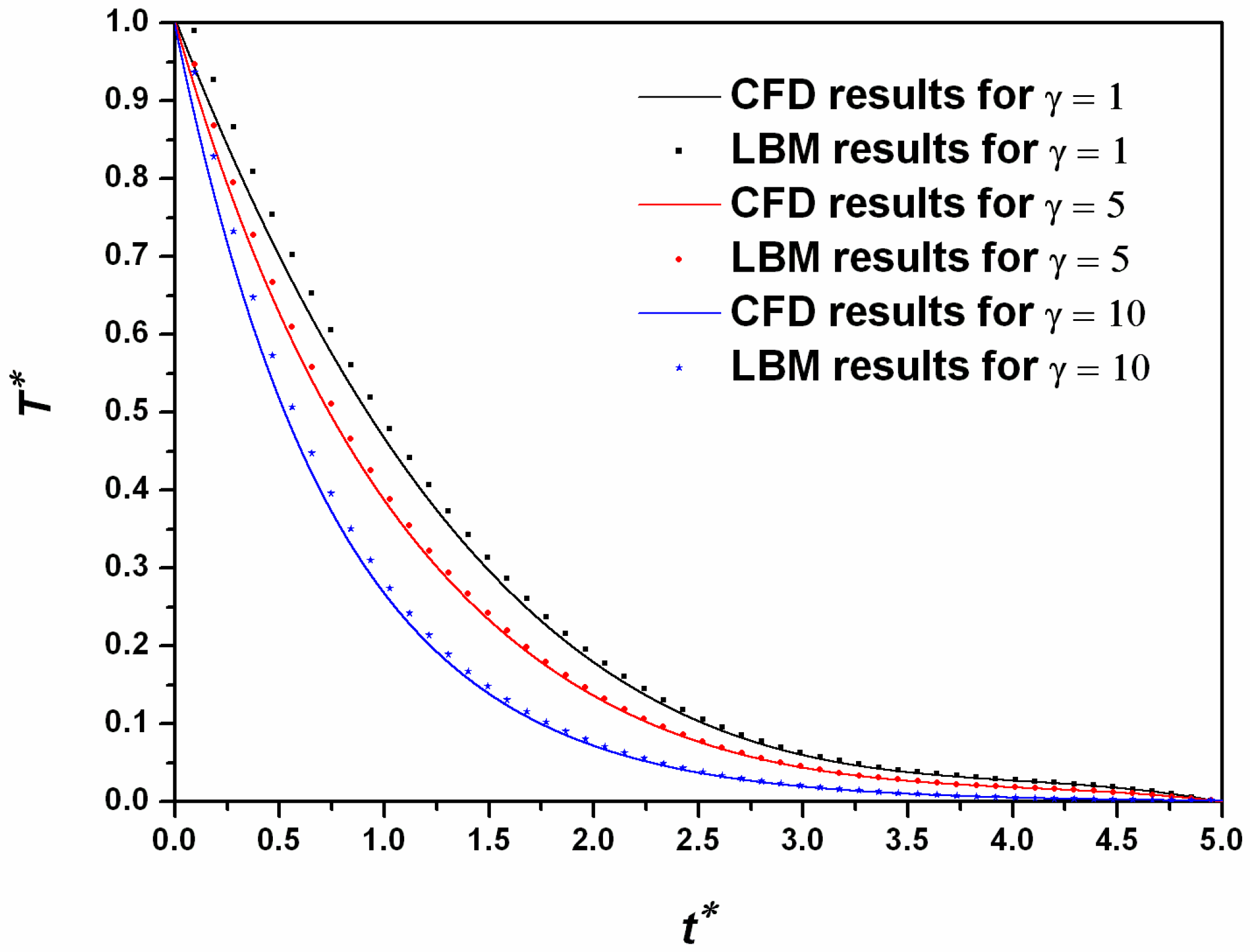
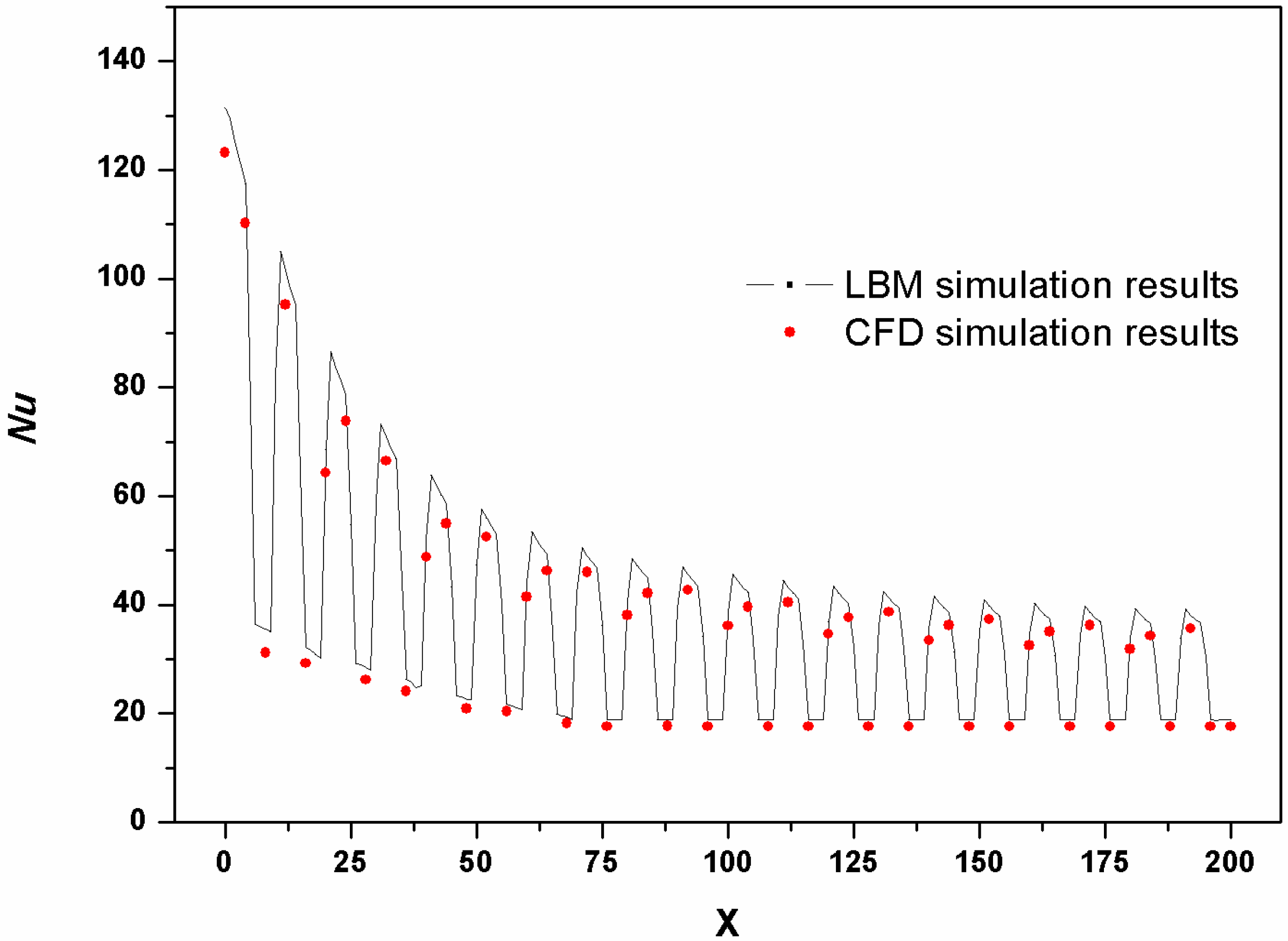
4.4. Model Validation

In the sake of validating the simulation results, these channel flows with smooth surface and rough surface were also simulated with the CFD model, described in the character 3, and the results compared.
Figure 6. Dimensionless temperature distributions of channel flow with smooth surfaces at the 400th step ( G = 0.6 ).
Energies 08 05704 g006
Figure 7. Dimensionless temperature distributions of channel flow with rough surfaces at the 400th step ( G = 0.6 ).
Energies 08 05704 g007
The local Nusselt number, an important indicator for monitoring the heat transfer performance, was calculated by follows:
N u = 1 κ ( T T w a l l ) L ( T b u l k T w a l l ) δ x
where T is the temperature of the lattice located nearest to the wall surface, T b u l k is the fluid bulk temperature at the current step, L is the flow distance.
The flow direction Nu distributions obtained by the LB method and CFD theory are presented in Figure 8. It can be observed that both the CFD and LBM produce similar results, where the variation trends predicted by these two models are consistent and the values shows a satisfactory agreement with the maximum error of about 8%. This validation result indicated that the LBM model presented in the paper could be used to describe the fluid flow and heat transfer performance.
Figure 8. The flow direction Nu distributions obtained by the LB method and CFD theory (simulation conditions: G t = 0.2 , contact angle θ = 131.38°, G = 0.6 ).
Energies 08 05704 g008

4.5. Quantitative Analysis and Discussion

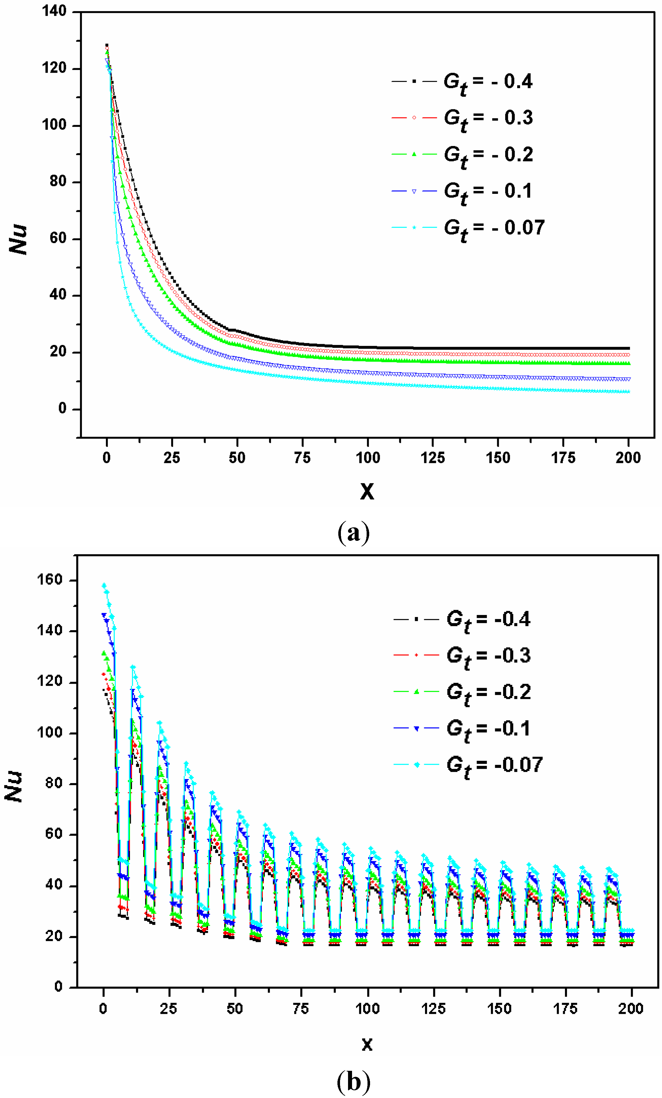
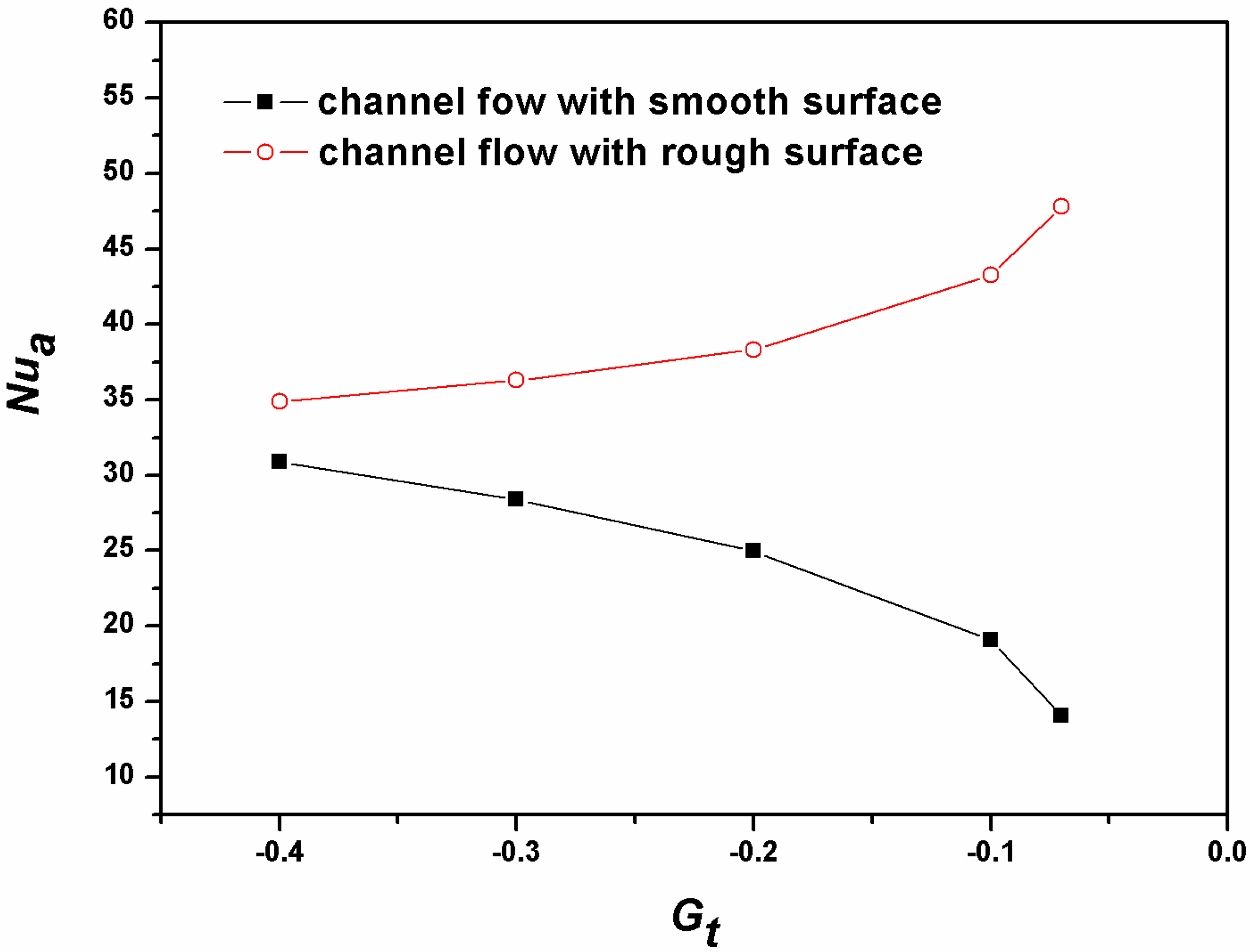
4.5.1. Heat Exchanger Performance

Figure 9 shows the local Nusselt number variation along the flow direction at the steady state with two types of surface microstructures, with G t ranging from −0.4 to −0.07. It can be seen that the local heat transfer intensity is high at the inlet, and the intensity decreases with the fluid going downstream and gradually approaching a constant stage. This is because the downstream temperature difference between the working fluid and wall is low compared to that at the entry region, in other words, the heat exchange driving force is lower approaching the exit. Apart from the above local Nusselt distribution analysis, the flow direction averaged Nusselt number, N u a , is a more direct way for one to evaluate the overall heat exchange intensity.
Figure 9. Local Nusselt number along the flowing direction for the channel flow with (a) smooth surfaces and (b) roughness surfaces ( G = 0.6 ).
Energies 08 05704 g009
The flow direction averaged Nusselt number with different values of G t is shown in Figure 10, where three points can be observed: (1) in the channel flow with smooth surface, the Nusselt number becomes smaller with increasing G t ; (2) in the channel flow with rough surface, the Nusselt number gets larger with increasing G t , namely, using the hydrophobic surface, the heat transfer performance will be worse in case of smooth-surface flow but improved in the case of rough-surface flow; and (3) the heat transfer performance can be enhanced when the smooth surface is displaced by the rough surface no matter what the surface wettabilities are. In the following content, a detailed analyses of these three aspects will be described. Primarily, as to the smooth-surface flow, if the surface hydrophobic characteristics are better, the attractive force of the fluid/solid interaction is small owing to low surface energy.
Figure 10. Averaged Nusselt number at the steady state for the channel flow with different surfaces ( G = 0.6 ).
Energies 08 05704 g010
This force can be easily destroyed by the fluid shear stresses and the slip velocity at the fluid/solid interface with the same direction as that of the mainstream is formed, which leads to the increased speed of the flow, as shown in Figure 11a. That is to say, the velocity of the liquid-phase flow is larger when the hydrophobic properties are better. The flow time is therefore less for the hydrophobic-surface channel flow if the flow length is the same, making the heat transfer insufficient compared with the hydrophilic-surface channel flow. In addition, the liquid will disconnect from the walls more easily with the improved hydrophobic properties. A special case is the ideal-superhydrophobic-surface channel flow where G = 0.07 . Theoretically, liquid will not stick to the surface and a very thin gas film is formed in between the fluid and the solid surface, as shown in Figure 11b. This phenomenon can be also observed from our simulations. In that case, the heat exchange between the liquid and solid wall is insufficient because the gas film plays the role of the heat insulating layer since the thermal conductivity of the gas is relatively small compared to that of the liquid. The local enlarged details of the phase interface and the temperature distribution for the hydrophilic-surface flow and superhydrophobic-surface flow are provided in Figure 12. We can see the liquid temperature in the case of G t = 0.4 is lower than that in the case of G t = 0.07 . These above points can explain why the heat transfer performance is worsened when the hydrophobic surface is adopted for the smooth-surface channel flow.
Secondly, as to the rough-surface channel flow, the situation is reversed: the better the hydrophobic surface is, the better the heat transfer performance becomes. This can be analyzed from the point of view of the heat transfer mechanism, which is closely related to the flow behavior. The phase interface, streamline and temperature distribution for the channel flow with rough surfaces are provided in Figure 13. If the surface is hydrophilic, liquid sinks into the grooves; as shown in Figure 13(1a); if the hydrophobic properties of a surface are to be better, the depth that the liquid penetrates into the grooves among the roughness bumps becomes lesser and the volume of liquid which flows into the grooves is also reduced; and if the surface is superhydrophobic, according to the research of Öner [9] and Extrand [10], the liquid will sweep over the roughness bumps without any contact with the solid surface. Our simulation agrees with this theoretical model well, as shown in Figure 13(2a). It can be found from the streamlines that in the case of hydrophilic-surface flow, there is no flow in the grooves; but in the case of superhydrophobic-surface flow, vortexes can be observed in the grooves. This is because, in present simulation, the velocity of the main flow is not large enough to drive the liquid to move but it is big enough to make the gas mass form vortexes since the viscosity of the gas is smaller than that of the liquid ( ξ = 10 ). Thus, within the grooves, the heat exchange mechanisms in the case of hydrophilic-surface flow and in case of superhydrophobic-surface flow correspond to heat conduction and heat convection, respectively. Normally, the heat exchange performance of the later is superior to that of the former. This can be also observed from the Figure 13(1c) and Figure 13(2c), where the heat transfer performance in the case of G t = 0.07 is better than that in the case of G t = 0.4 .
Figure 11. (a) Slip flow at the fluid/solid interface for a hydrophobic surface and (b) theoretical model for an ideal superhydrophobic surface.
Energies 08 05704 g011
Figure 12. The local enlargement of (a) phase interface and (b) temperature distribution for the channel flow with smooth surfaces when (1) G t = 0.4 , G = 0.6 and (2) G t = 0.07 , G = 0.6 .
Energies 08 05704 g012
Figure 13. (a) Phase interface; (b) streamline and (c) temperature distribution for the channel flow with rough surface when (1) G t = 0.4 , G = 0.6 and (2) G t = 0.07 , G = 0.6 .
Energies 08 05704 g013
Finally, the heat exchange performance of the rough-surface flow always exceeds that of smooth-surface flow. The reasons differ with the variation of the surface wettabilities. When the hydrophilic surface is used, it is because of the addition of the heat exchange area, however, this explanation will not be appropriate for the hydrophobic-surface flow. In that situation, the enhanced heat exchange can be attributed to the vortex motion of the gas mass within the grooves.

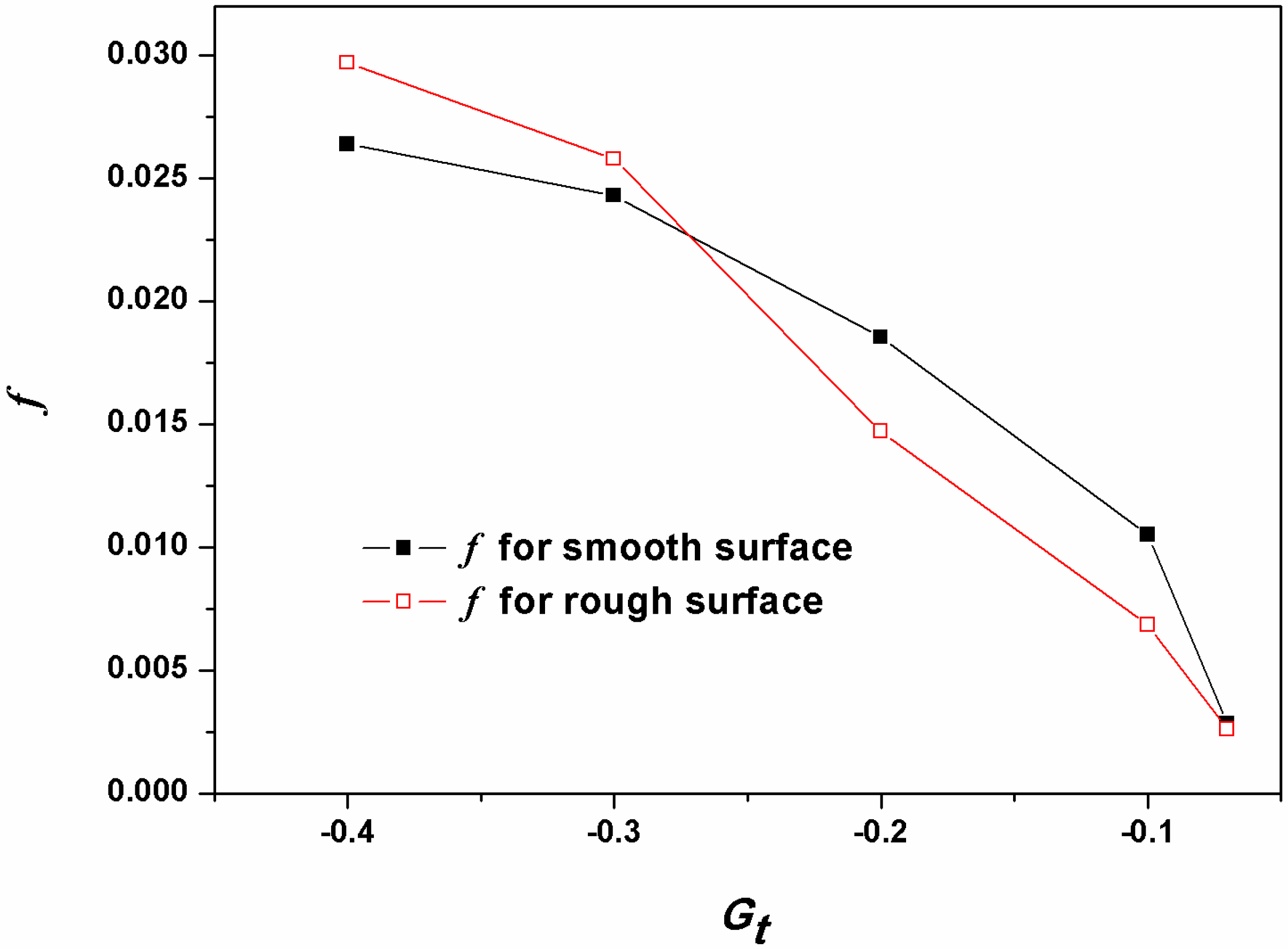
4.5.2. Pressure Drop

When flows reach the steady state, the frictional resistance coefficient, given by Equation (24), is calculated to measure the pressure drop, where the smaller the coefficient is, the lesser the pressure loss is:
f = 2 Δ p d / ( | u | 2 ρ l )
where d is the channel size, l is the flow distance of liquid in x direction, |u| is the average magnitude of velocity, ρ is the density of liquid and Δ p is the pressure drop between inlet and outlet sections.
The frictional resistance coefficient of channel flow with smooth and rough surfaces is illustrated in Figure 14. Compared to the hydrophilic-surface flow, the frictional resistance coefficient for the hydrophobic-surface flow is much less because of its lower surface energy. It can be found from Figure 6 that, for the smooth-surface flow, a very thin gas film is formed between the fluid and superhydrophobic wall and the liquid/solid interface is replaced by the gas/liquid one, while from Figure 7, it can be observed that, for the rough-surface flow, liquid sweeps over the grooves and the contact area is reduced in the case of hydrophobic-surface flow. Consequently, the friction is rapidly decreased.
In addition, for the hydrophobic surface (|Gt| < 0.32), the friction resistance coefficient of flow over a rough surface is less than that over a smooth surface, while for the hydrophilic surface (|Gt| > 0.32), this coefficient for the rough surface is larger than that for smooth surface The most likely reason is that the roughness elements increase the contact area for a hydrophilic surface but decrease it for a hydrophobic one. The details can be found in Figure 6 and Figure 7.
Figure 14. Frictional resistance coefficient of channel flow for smooth and rough surfaces ( G = 0.6 ).
Energies 08 05704 g014

5. Conclusions

The surface wettability and roughness have a significant impact on the fluid flow behavior and heat transfer performance in microfluidic channels. In this paper, the lattice Boltzmann method, as an alternative numerical approach on mescoscopic level between the traditional macroscopic CFD and the microscopic molecular dynamics (MD) methods, is used to investigate the heat exchange performance when a hot liquid flows through cold channels with different wettabilities and topographical surfaces. The double-distribution function (DDF) two-phase thermal lattice Boltzmann BGK (LBGK) model is applied, where the Shan-Chen multiphase LBGK model is used to describe the flow field and the independent distribution function is introduced to solve the temperature field. According to the simulation results, some main conclusions can be drawn as follows:
(1)
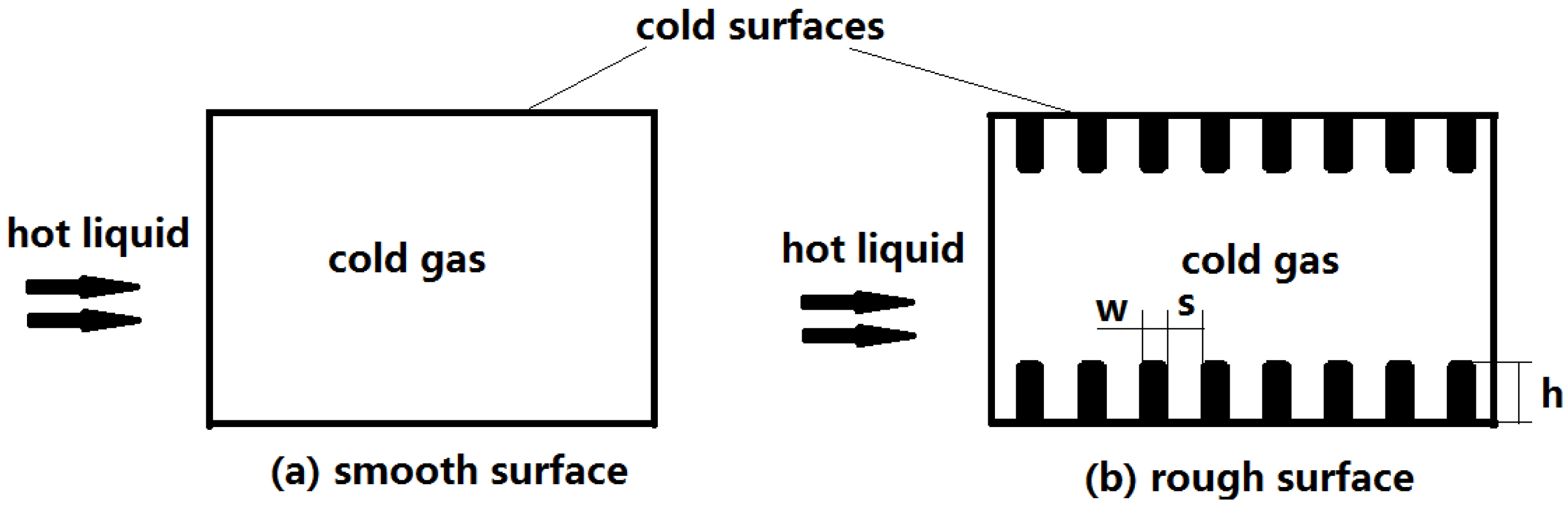
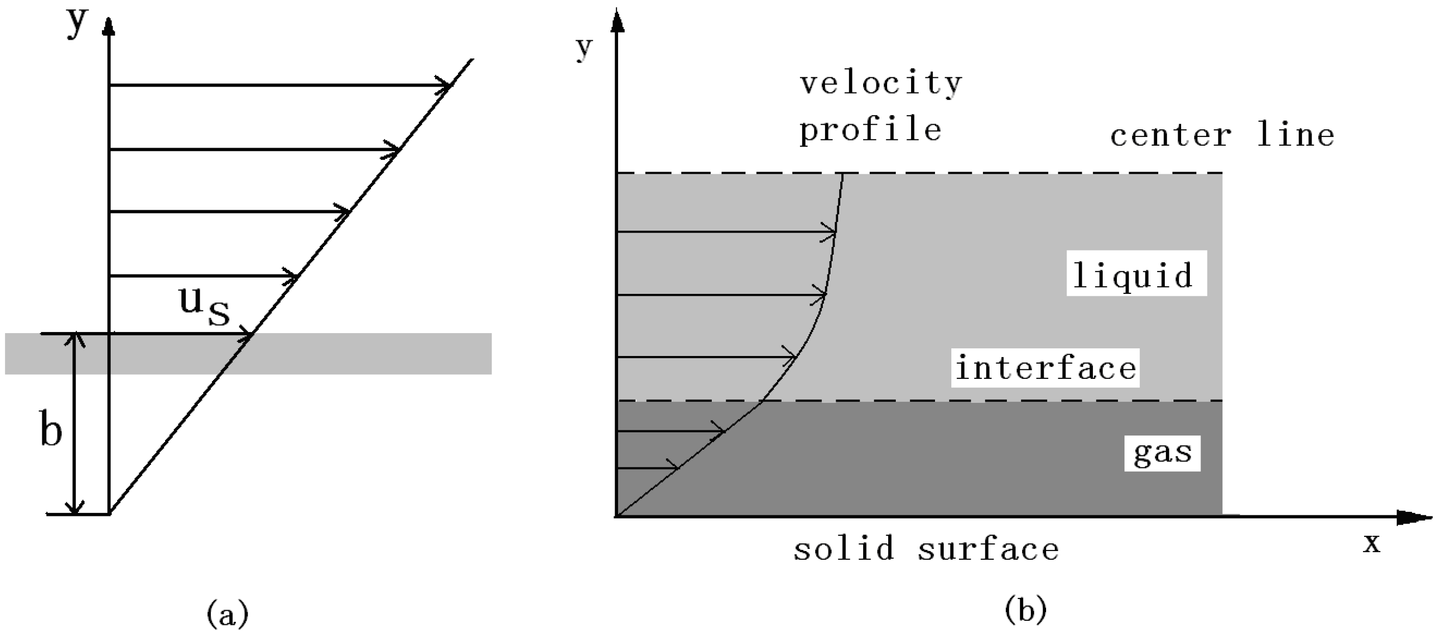
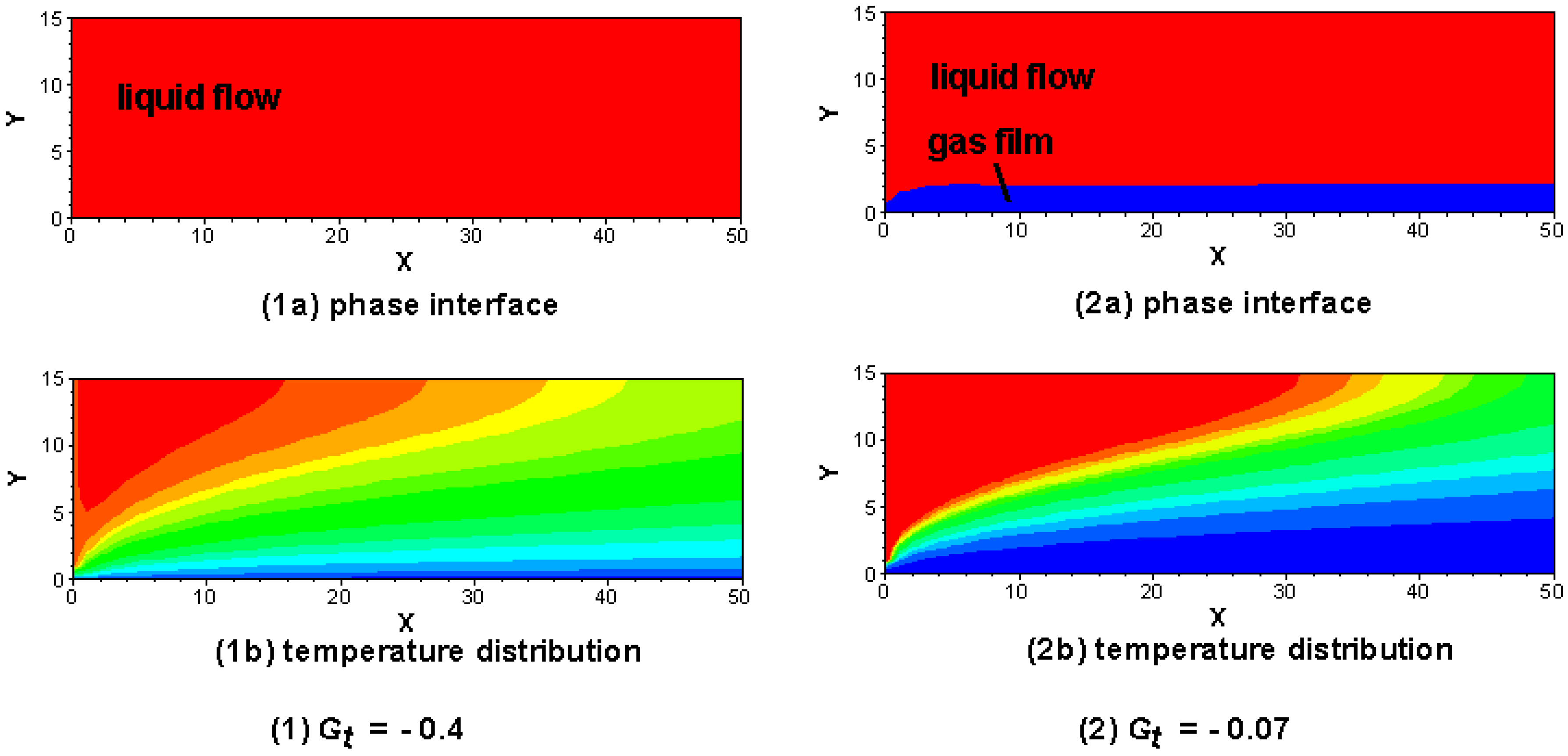
For the smooth-surface channel flow, the pressure drop could be reduced by using hydrophobic surfaces because a very thin gas film is formed between the fluid and superhydrophobic wall and the liquid/solid interface is replaced by a gas/liquid one. However the heat transfer performance is worsened when the surface is hydrophobic compared to the hydrophilic surface flow. This is because that the velocity of liquid-phase flow is larger when the hydrophobic properties are better. The flow time is therefore less for the hydrophobic-surface channel flow, masking the heat transfer insufficient compared with the hydrophilic-surface channel flow.
(2)
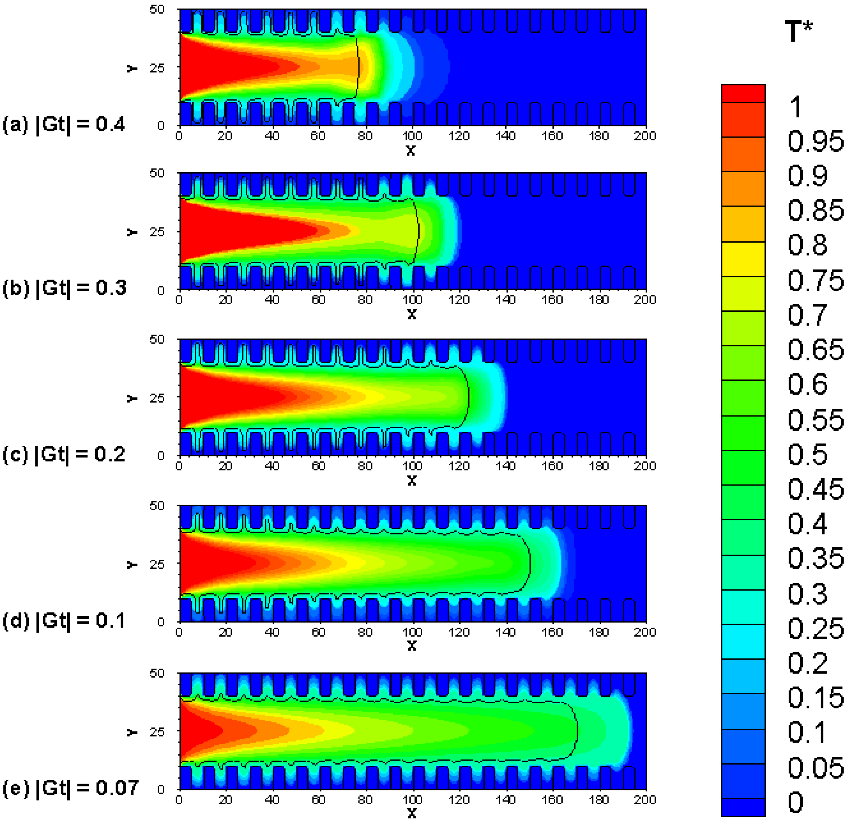
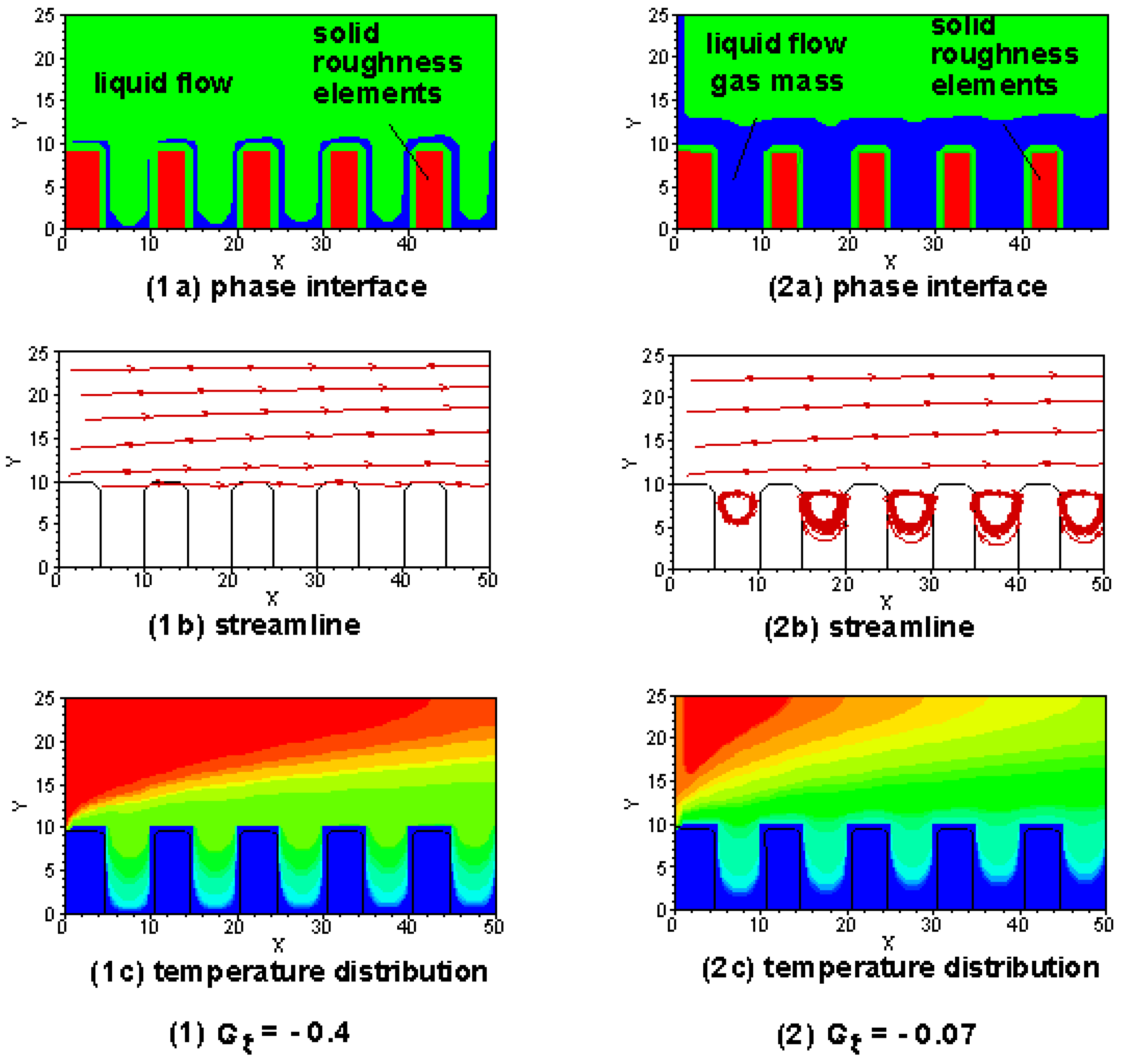
As to the rough-surface channel flow, the pressure drop for the hydrophobic-surface flow is much less because the liquid sweeps over the grooves and the contact area is reduced in the case of hydrophobic-surface flow. Moreover, the better the hydrophobic surface is, the better the heat transfer performance becomes. For the superhydrophobic surface channel flow, liquid sweeps over the roughness bumps and gas squeezes into the spaces and being subject to vertical movement owing to the drag force at the top side of the gap caused by the liquid flow in the main region, which will produce heat convection, a superior kind of heat exchange mechanism, to enhance the heat transfer performance.

Acknowledgments

The research work was supported by National Natural Science Foundation of China under Grant No. 51206179, the Central College Foundation of CAUC under Grant No. ZXH2012C001 and the Scientific Research Foundation of CAUC under Grant No. 2011QD22X.

Author Contributions

Jing Cui conceived and designed the numerical simulation and performed the numerical simulation; Yanyu Cui analyzed the data and revised the manuscript.

Conflicts of Interest

The authors declare no conflict of interest.

References

  1. Zhang, J.; Kwok, D.Y. Contact line and contact angle dynamics in superhydrophobic channels. Langmuir 2006, 22, 4998–5004. [Google Scholar] [CrossRef] [PubMed]
  2. Jeffs, K.; Maynes, D.; Webb, B.W. Prediction of turbulent channel flow with superhydrophobic walls consisting of micro-ribs and cavities oriented parallel to the flow direction. Int. J. Heat Mass Transf. 2010, 53, 786–796. [Google Scholar] [CrossRef]
  3. Chibbaro, S.; Costa, E.; Dimitrov, D.I.; Diotallevi, F.; Milchev, A.; Palmieri, D.; Pontrelli, G.; Succi, S. Capillary Filling in Microchannels with Wall Corrugations: A Comparative Study of the Concus-Finn Criterion by Continuum, Kinetic, and Atomistic Approaches. Langmuir 2013, 25, 12653–12660. [Google Scholar] [CrossRef] [PubMed]
  4. Lauga, E.; Stone, H.A. Effective slip in pressure-driven Stokes flow. J. Fluid Mech. 2003, 489, 55–77. [Google Scholar] [CrossRef]
  5. Ybert, C.; Barentin, C.; Cottin-Bizonne, C.; Joseph, P.; Bocquet, L. Achieving large slip with superhydrophobic surfaces: Scaling laws for generic geometries. Phys. Fluids 2013, 19, 123601. [Google Scholar] [CrossRef]
  6. Davies, J.; Maynes, D.; Webb, B.W.; Woolford, B. Laminar flow in a microchannel with superhydrophobic walls exhibiting transverse ribs. Phys. Fluids 2006, 18, 087110. [Google Scholar] [CrossRef]
  7. Ou, J.; Perot, B.; Rothstein, J.P. Laminar drag reduction in microchannels using ultrahydrophobic surfaces. Phys. Fluids 2004, 16, 4635. [Google Scholar] [CrossRef]
  8. Cui, J.; Li, W.; Lam, W.H. Numerical investigation on drag reduction with superhydrophobic surfaces by lattice-Boltzmann method. Comput. Math. Appl. 2011, 61, 3678–3689. [Google Scholar] [CrossRef]
  9. Öner, D.; McCarthy, T.J. Ultrahydrophobic surfaces. Effects of topography length scales on wettability. Langmuir 2000, 16, 7777–7782. [Google Scholar] [CrossRef]
  10. Extrand, C.W. Model for contact angles and hysteresis on rough and ultraphobic surfaces. Langmuir 2002, 18, 7991–7999. [Google Scholar] [CrossRef]
  11. Wenzel, R.N. Resistance of solid surfaces to wetting by water. Ind. Eng. Chem. 1936, 28, 988–994. [Google Scholar] [CrossRef]
  12. Cassie, A.B.D.; Baxter, S. Wettability of porous surfaces. Trans. Faraday Soc. 1944, 40, 546–551. [Google Scholar] [CrossRef]
  13. Alexander, F.J.; Chen, S.; Sterling, J.D. Lattice boltzmann thermohydrodynamics. Phys. Rev. E 1993, 47, 2249–2252. [Google Scholar] [CrossRef]
  14. Chen, Y.; Ohashi, H.; Akiyama, M. Thermal lattice Bhatnagar-Gross-Krook model without nonlinear deviations in macrodynamic equations. Phys. Rev. E 1994, 50, 2776–2783. [Google Scholar] [CrossRef]
  15. Bartoloni, A.; Battista, C.; Gabasino, S.; Paolucci, P.S. LBE simulations of Rayleigh-Bénard convection on the APE100 parallel processor. Int. J. Mod. Phys. C 1993, 4, 993–1006. [Google Scholar] [CrossRef]
  16. Shan, X. Simulation of Rayleigh-Benard convection using a lattice Boltzmann method. Phys. Rev. E 1997, 55, 2780–2788. [Google Scholar] [CrossRef]
  17. He, X.; Chen, S.; Doolen, G.D. A Novel Thermal Model for the Lattice Boltzmann Method in Incompressible Limit. J. Comput. Phys. 1998, 146, 282–300. [Google Scholar] [CrossRef]
  18. Gunstensen, A.K.; Rothman, D.H.; Zaleski, S.; Zanetti, G. Lattice Boltzmann model of immiscible fluids. Phys. Rev. A 1991, 43, 4320–4327. [Google Scholar] [CrossRef] [PubMed]
  19. Swift, M.R.; Osborn, W.R.; Yeomans, J.M. Lattice Boltzmann simulation of nonideal fluids. Phys. Rev. Lett. 1995, 75, 830–833. [Google Scholar] [CrossRef] [PubMed]
  20. Swift, M.R.; Orlandini, E.; Osborn, W.R.; Yeomans, J.M. Lattice Boltzmann simulations of liquid-gas and binary fluid systems. Phys. Rev. E 1996, 54, 5041–5052. [Google Scholar] [CrossRef]
  21. Luo, L.S. Unified theory of lattice Boltzmann models for nonideal gases. Phys. Rev. Lett. 1998, 81, 1618–1621. [Google Scholar] [CrossRef]
  22. Luo, L.S. Some recent results on discrete velocity models and ramifications for lattice Boltzmann equation. Comput. Phys. Commun. 2000, 129, 63–74. [Google Scholar] [CrossRef]
  23. He, X.; Chen, S.; Zhang, R. A lattice Boltzmann scheme for incompressible multiphase flow and its application in simulation of Rayleigh-Taylor instability. J. Comput. Phys. 1999, 152, 642–663. [Google Scholar] [CrossRef]
  24. Qian, Y.H.; d'Humieres, D.; Lallemand, P. Lattice BGK models for Navier-Stokes equation. EPL (Europhys. Lett.) 1992, 17, 479. [Google Scholar] [CrossRef]
  25. Bhatnagar, P.L.; Gross, E.P.; Krook, M. A model for collision processes in gases. I. Small amplitude processes in charged and neutral one-component systems. Phys. Rev. 1954, 94, 511–525. [Google Scholar] [CrossRef]
  26. Raiskinmäki, P.; Shakib-Manesh, A.; Jasberg, A.; Koponen, A.; Merikoski, J.; Timonen, J. Lattice-Boltzmann simulation of capillary rise dynamics. J. Stat. Phys. 2002, 107, 143–158. [Google Scholar] [CrossRef]
  27. Hyväluoma, J.; Raiskinmäki, P.; Jäsberg, A.; Koponen, A.; Kataja, M.; Timonen, J. Evaluation of a lattice-Boltzmann method for mercury intrusion porosimetry simulations. Future Gener. Comput. Syst. 2004, 20, 1003–1011. [Google Scholar] [CrossRef]
  28. Chopard, B.; Droz, M. Cellular Automata Modeling of Physical Systems; Cambridge University Press: Cambridge, UK, 1998. [Google Scholar]
  29. Frisch, U.; Hasslacher, B.; Pomeau, Y. Lattice-gas automata for the Navier-Stokes equation. Phys. Rev. Lett. 1986, 56, 1505–1508. [Google Scholar] [CrossRef] [PubMed]
  30. Wang, M.; Pan, N. Modeling and prediction of the effective thermal conductivity of random open-cell porous foams. Int. J. Heat Mass Transf. 2008, 51, 1325–1331. [Google Scholar] [CrossRef]

