2.1. Design of Experiments
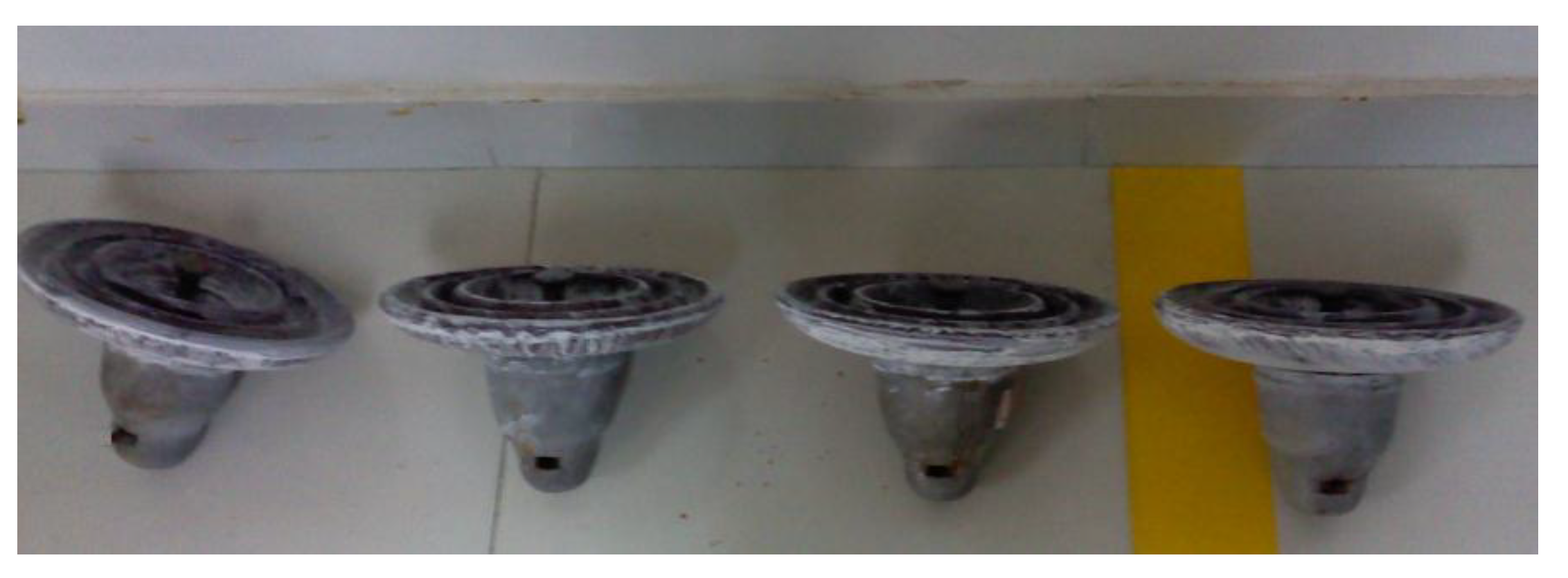
Artificial contamination experiments were carried out in high-voltage laboratory of Shenzhen Power Supply Bureau. In practice, insulators in same string have the similar contamination grades. Recognition result of one insulator can reflect the contamination severity of the whole string. Hence, the study subject can be set as single piece of insulator. Twelve pieces of cap and pin type suspension ceramic insulators of type XP-70 (Dalian Insulator Group Co., Ltd., Dalian, China were used in the experiments. The top surface of XP-70 is 674 cm
2, the bottom surface is 917 cm
2, the creepage distance is 295 cm and the rated voltage is 10 kV. Artificially contaminated insulators are shown in
Figure 3.
Figure 3.
Artificially contaminated insulators used in experiments.
Figure 3.
Artificially contaminated insulators used in experiments.
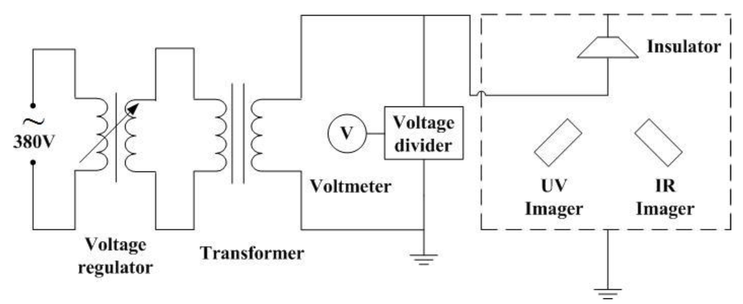
The test system is shown in
Figure 4. Voltmeter and voltage regulator are integrated in a test transformer control box, which controls the operating voltage. Output of the transformer (type GS108, China Electric Equipment Group, Nanjing, China) was connected to the steel nail on the underneath of insulator by a copper wire. And the earth wire was connected to the steel cap. Wires used in experiments were compressed tightly to avoid any discharge caused by poor contact.
Figure 4.
Schematic diagram of the test circuit.
Figure 4.
Schematic diagram of the test circuit.
Before the tests, all insulator samples were carefully washed using running water to remove feculence and dried naturally. After the preparation, solid layer method based on IEC 60507 standard was adopted to produce uniform pollution layers on the surface of insulators. The artificial pollutant was made of distilled water, kaolin (substitute for non-soluble substances in natural contaminants) and sodium chloride (NaCl, substitute for soluble salts in natural contaminants). In order to simulate the four contamination grades (I, II, III, IV), insulator samples were divided into four groups. There were three insulators in each group. Values of salt deposit density (SDD) of each group were selected as 0.03–0.06 mg/cm2 (corresponding to grade I), 0.06–0.1 mg/cm2 (corresponding to grade II), 0.1–0.25 mg/cm2 (corresponding to grade III) and 0.25–0.35 mg/cm2 (corresponding to grade IV). Value of non-soluble deposit density (NSDD) was set as 1 mg/cm2 for every group. Amounts of sodium chloride and kaolin were calculated by the surface area of insulator, SDD and NSDD. The pollutants were brushed on the surface of insulators uniformly and shady dried for 24 h before the high voltage experiments. In 110 kV transmission line, phase voltage applied to an insulator string with six or seven pieces of insulators is 63.5 kV. In order to simulate the practical situation as far as possible, the test voltage was set as 10 kV, which is the average voltage for a suspension insulator in 110 kV transmission line (10 kV is also the rated voltage of XP-70). When relative humidity (RH) is less than 75%, soluble salt in contaminate does not dissolve obviously and the leakage current value is small. So the temperature rise and discharge on insulator surface are not obvious. In order to simulate insulators at relatively high humidity conditions, the experiments were carried out at relative humidity of 80%, 85% and 90%, respectively. The permissible variance range of RH was ±2%. Ambient temperature was recorded in synchronization with the shooting of IR image.
2.2. Shooting and Preprocessing of Infrared (IR) Images
According to [
6,
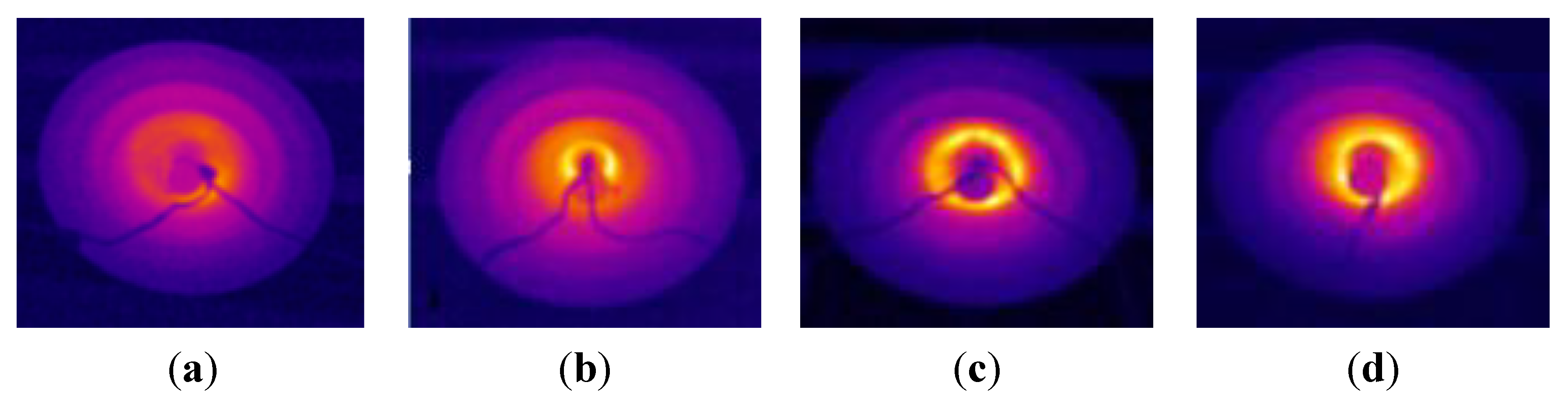
7], compared with other parts of suspension insulator, temperature rise on the underneath is most obvious and suitable for subsequent analysis and processing. IR images of the underneath of XP-70 suspension insulators were shot at a distance of 2 m by Ti-32 IR imager (Fluke Corporation, Everett, WA, USA). Color palette option of IR imager was set as “Iron Oxide Red”. According to [
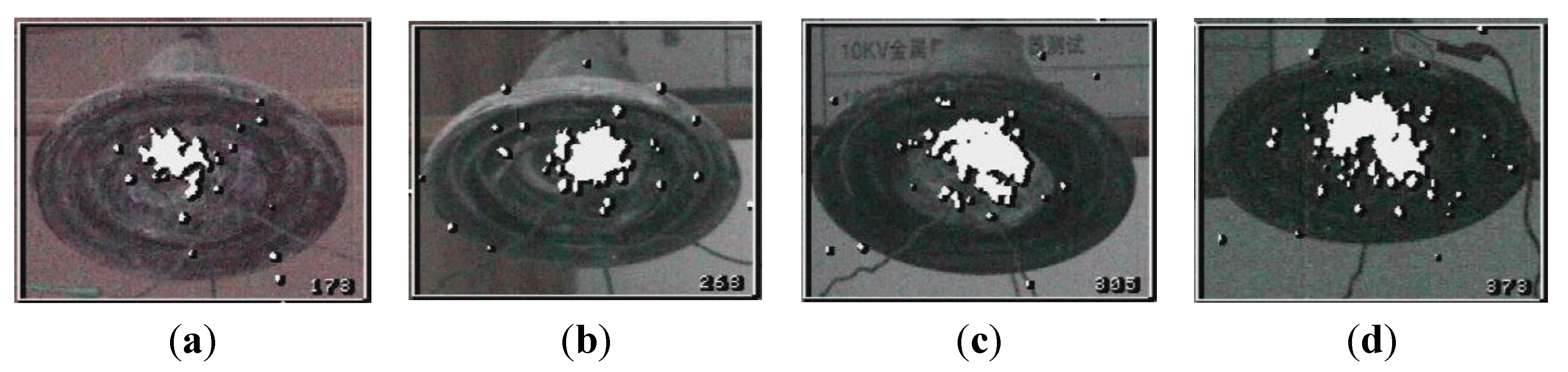
5], it takes about 2 h for a polluted disc suspension insulator to achieve thermal balance. Therefore, IR image shooting was started 2 h later than the beginning of high voltage experiment. Five pieces of IR image of each contamination grade were shot at an interval of 5 min. IR images of insulators with different contamination grades at 85% RH are shown in
Figure 5.
Figure 5.
Infrared images of polluted insulators at 85% RH; (a) Insulator of I contamination grade; (b) Insulator of II contamination grade; (c) Insulator of III contamination grade; and (d) Insulator of IV contamination grade.
Figure 5.
Infrared images of polluted insulators at 85% RH; (a) Insulator of I contamination grade; (b) Insulator of II contamination grade; (c) Insulator of III contamination grade; and (d) Insulator of IV contamination grade.
Two files can be obtained from the IR imager. One is IR image in BMP format. The other is temperature data table in Excel format. The size of image and Excel file is 320 × 240. Temperature data of the insulator region is the basis of subsequent analysis. It requires two steps to obtain the temperature data of insulator. The first step is segmenting the insulator from background on IR image and recording the coordinates of insulator region. The second step is reading the corresponding temperature data from Excel file according to the recorded coordinates.
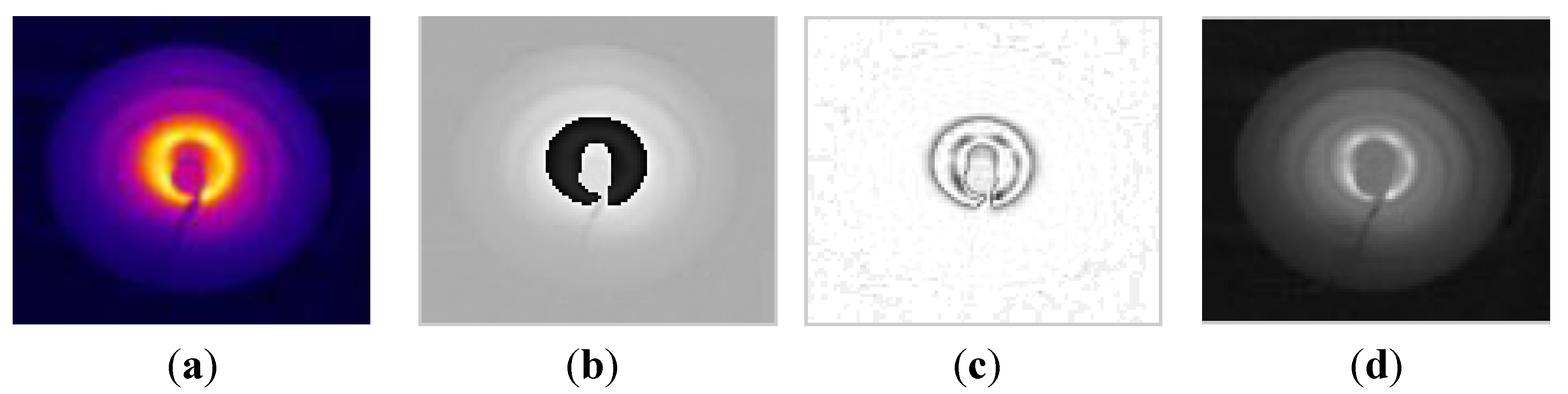
HSI color standard is a common standard for color image display. Hue (H), saturation (S) and intensity (I) are used to display a color image in HSI color space. In order to look for the proper component image for segmentation, HSI component images of IR image are compared in
Figure 6.
Figure 6.
Comparison of images in HSI color space; (a) IR image of insulator; (b) H component image; (c) S component image; and (d) I component image.
Figure 6.
Comparison of images in HSI color space; (a) IR image of insulator; (b) H component image; (c) S component image; and (d) I component image.
As is shown in
Figure 6, it is hard to distinguish the region of insulator from background in H or S component image. Meanwhile, insulator contour of I component image is relatively clear. Hence I component image was adopted to extract the region of insulator using image segmentation algorithm. In this paper, a mathematical morphology improved Otsu algorithm was proposed to realize the image segmentation. At first, Otsu algorithm was applied to the preliminary segmentation of I component image. After that, further morphological processing was utilized to improve segmentation effect.
Otsu algorithm is a kind of high efficiency image segmentation algorithm, which has the ability to divide object from background without any prior knowledge. Supposing the size of image is
M ×
N, pixel number of the object is
N1, pixel number of the background is
N2. Area proportion of object to entire image is shown in Equation (2):
And area proportion of background to entire image is shown as:
The overall average of gray value is defined in Equation (4):
where μ
1 is the average gray value of object and μ
2 is the average gray value of background. Variance of object and background is defined as:
Traversal method is adopted to obtain the proper segmentation threshold
T, which ensures that the value of variance g is the maximum of all possible values. Taking IR image of IV contamination grade insulator for example, binary image obtained from Otsu segmentation can be seen in
Figure 7b. In binary image, white area represents insulator surface, and black area represents background. As is shown in
Figure 7b, the extracted insulator surface is smaller than the actual one and the border is rough. In order to improve the segmentation effect, mathematical morphology methods were used to further process the preliminarily segmented image.
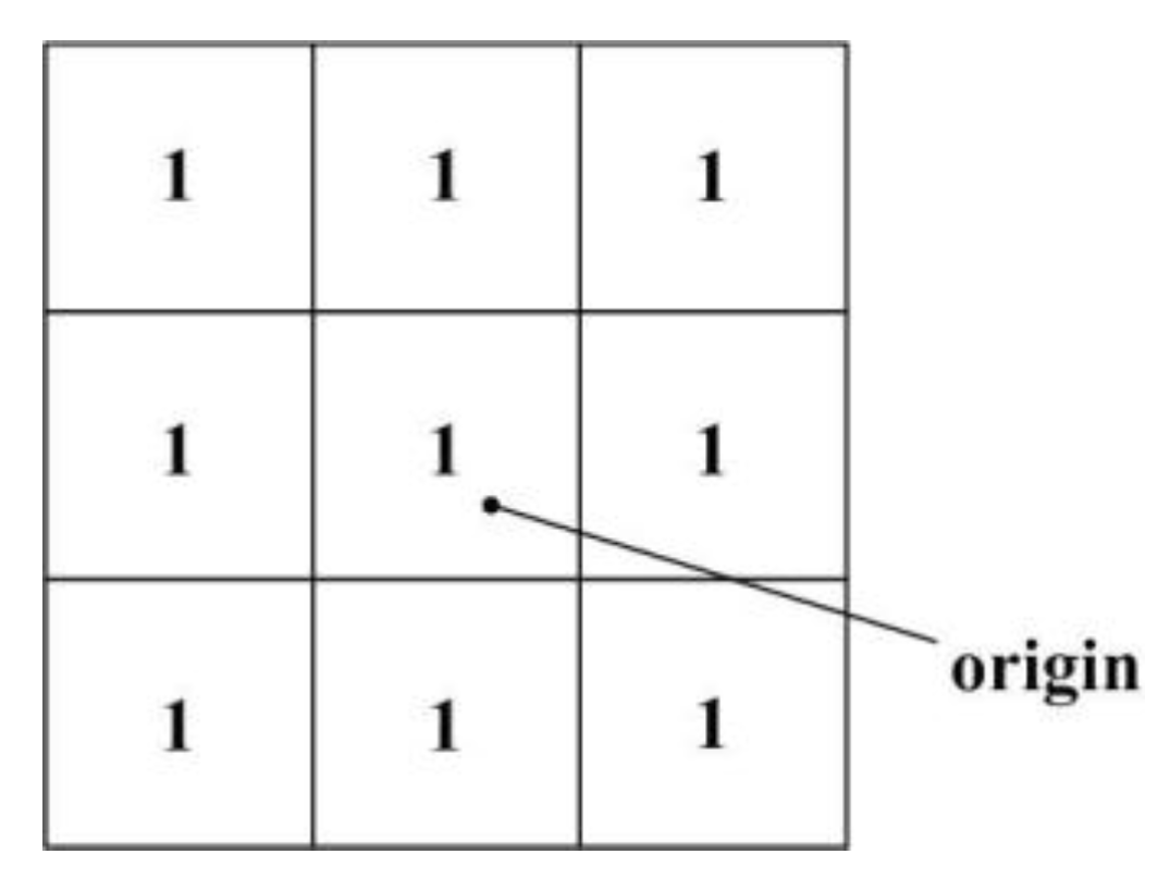
Mathematical morphology is a kind of image analysis methodology based on set theory. Dilation and erosion are two basic operations of mathematical morphology. Different combinations of dilation and erosion constitute various operations such as opening and closing. Size and shape of mathematical morphology is defined by structure element
B, which is constituted by 0 and 1. An example of square structure element with size of 3 × 3 is shown in
Figure 7.
Figure 7.
A square structure element with size of 3 × 3.
Figure 7.
A square structure element with size of 3 × 3.
The dilation operation of image
A using structure element
B is defined as:
When origin of structure element
B is located in point (
x,
y), if intersection of
B and
A is a nonempty set, point (
x,
y) is a part of dilated binary image
D(
A). Dilation leads to the expansion of image. Erosion is the dual operation of dilation. It is defined as follows:
When origin of structure element
B is located in point (
x,
y), if all points of
B belong to image
A, point (
x,
y) is a part of eroded binary image
E(
A). We can see that erosion leads to the shrinking of the image. Opening and closing are combinations of dilation and erosion. The opening operation of image
A using structure element
B is defined as:
The closing operation of image
A using structure element
B is defined as:
Dilation operation leads to the expansion of image outline. Erosion operation leads to the shrinking of the image outline. Opening operation has the ability to break narrow connections and eliminate tiny protrusions. Closing operation has the ability to bridge slender gaps and fill small holes. In our study, a square structure element with size of 10 × 10 was applied to morphological processing. In order to eliminate protrusions, gaps and holes on the surface of insulator, the binary image obtained from Otsu algorithm was processed by opening and closing. After that, the image was dilated to expand the surface area of insulator. As is shown in
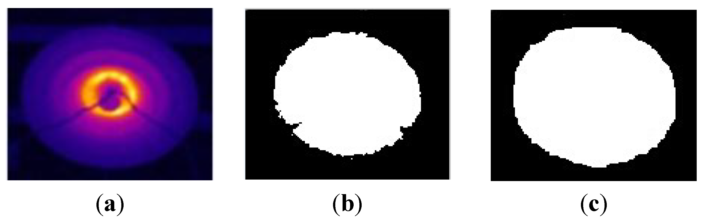
Figure 8c, morphological processing improves the segmentation effect significantly and the extracted insulator surface is close to the actual one.
Figure 8.
Result of image segmentation; (a) IR image of insulator; (b) Binary image after Otsu segmentation; and (c) Binary image after morphological processing.
Figure 8.
Result of image segmentation; (a) IR image of insulator; (b) Binary image after Otsu segmentation; and (c) Binary image after morphological processing.
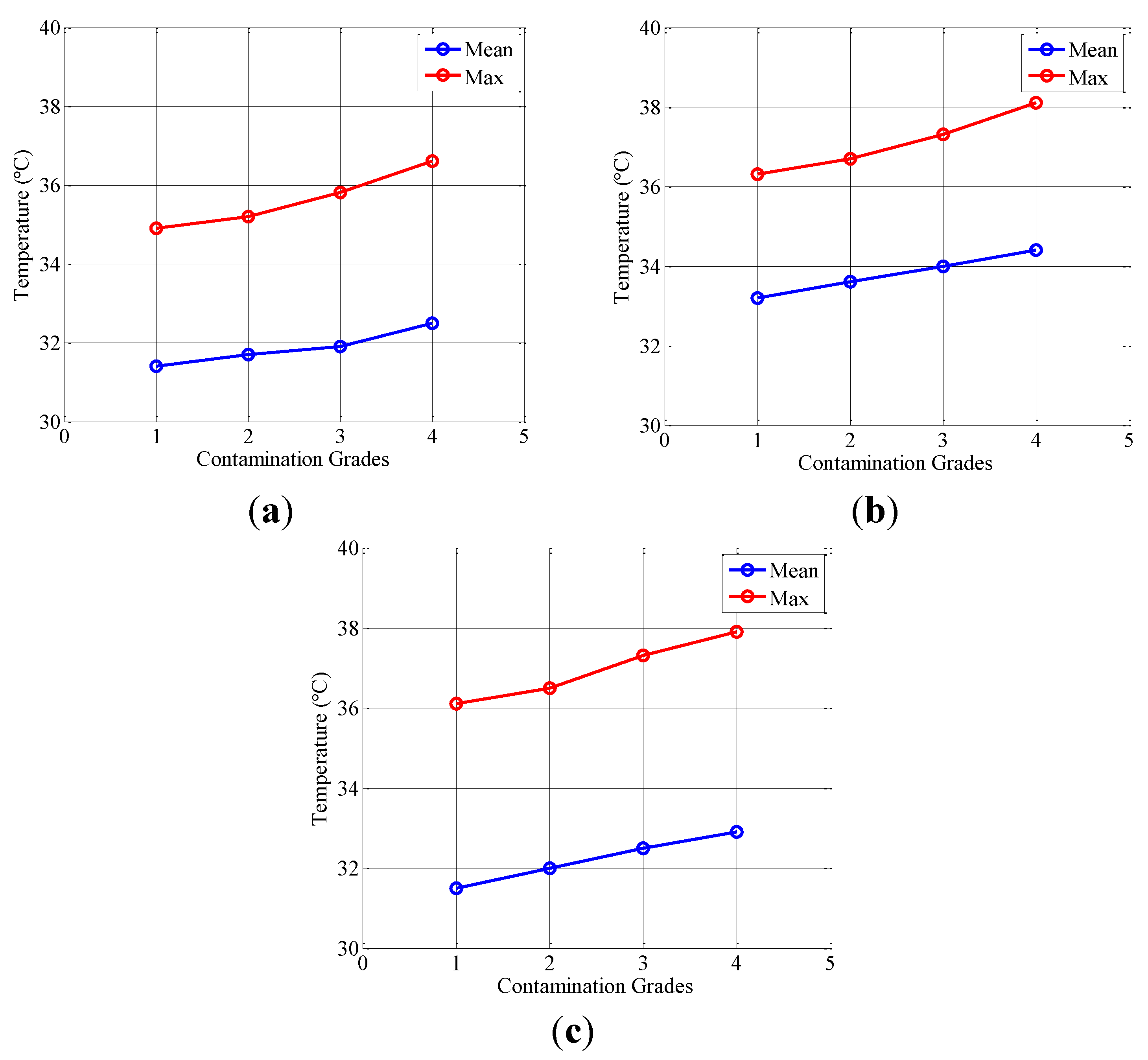
Distribution curves of mean temperatures and max temperatures of insulators with different contamination grades at different environment conditions (relative humidity and ambient temperature) are shown in
Figure 9. It can be seen that surface temperature of the contaminated insulator rises significantly in humid condition. Temperature rises of insulators with high contamination grades are more obvious than that of insulators with low contamination grades. As the temperature differences between each contamination grade are relatively small, it is difficult to establish a precise mathematical model between contamination grades and temperature characteristics. Therefore, artificial intelligent methodologies, such as information fusion and pattern recognition are applied to the contamination grades recognition in this study.
Figure 9.
Distribution curves of mean temperature and max temperature. (a) RH = 80%, ambient temperature is 29 °C; (b) RH = 85%, ambient temperature is 30.2 °C; (c) RH = 90%, ambient temperature is 28.3 °C.
Figure 9.
Distribution curves of mean temperature and max temperature. (a) RH = 80%, ambient temperature is 29 °C; (b) RH = 85%, ambient temperature is 30.2 °C; (c) RH = 90%, ambient temperature is 28.3 °C.
2.3. Shooting and Preprocessing of Ultraviolet (UV) Images
As mentioned in [
6,
7], area around steel nail on the underneath of an insulator has the highest current density and temperature rise. As a result of strong partial evaporation, dry bands appear around the steel nail and cause discharges [
23]. Meanwhile, in high voltage experiment, no continuous discharge can be observed by UV imager on the other parts of insulator. Therefore, the underneath of insulator is set as the objective of UV photography.
The type of UV imager used in this research is CoroCAM 504 (Council for Scientific and Industrial Research, Pretoria, South Africa). The UV imager was used in conjunction with a VDR-MC3 (Sony Group, Tokyo, Japan) video recorder. Output video format of the video recorder is vob. For the convenience of the subsequent process, vob-to-avi software was adopted to convert the video files from vob-to-avi format. Gain of the UV imager was set as 70%, threshold value was set as 40%, and photographic distance was 4 m. UV video shooting was synchronous with the shooting of IR image. Typical figures of UV images at 85% RH are shown in
Figure 10. In images, white spots represent the discharge intensity.
Figure 10.
Ultraviolet images of polluted insulators at 85% RH; (a) Insulator of I contamination grade; (b) Insulator of II contamination grade; (c) Insulator of III contamination grade; and (d) Insulator of IV contamination grade.
Figure 10.
Ultraviolet images of polluted insulators at 85% RH; (a) Insulator of I contamination grade; (b) Insulator of II contamination grade; (c) Insulator of III contamination grade; and (d) Insulator of IV contamination grade.
The UV videos were recorded at a rate of 25 frames per second. The size of UV image is 320 × 240. Electric discharges are displayed as white spots on UV images. Discharge intensity can be characterized by the number of white pixels (the area of white spots). In gray image, the gray values of white spots are close to 255. After analysis and comparison, gray value of 200 was selected as the threshold of white spot area calculation. Pixels with gray value larger than 200 were calculated as electric discharge white spots. And pixels with gray value smaller than 200 were considered background. According to this principle, pixel numbers of white spots were calculated for further processing.
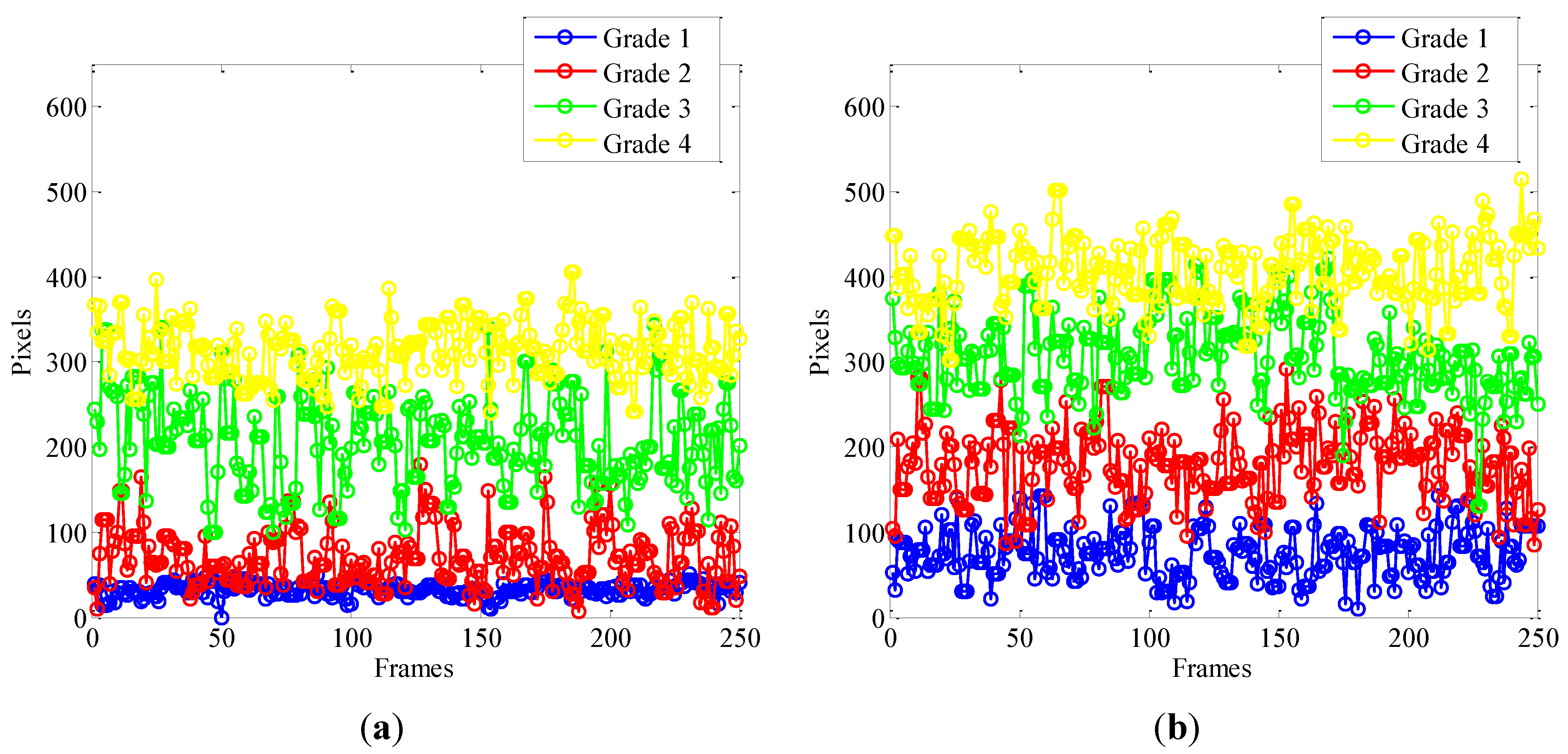
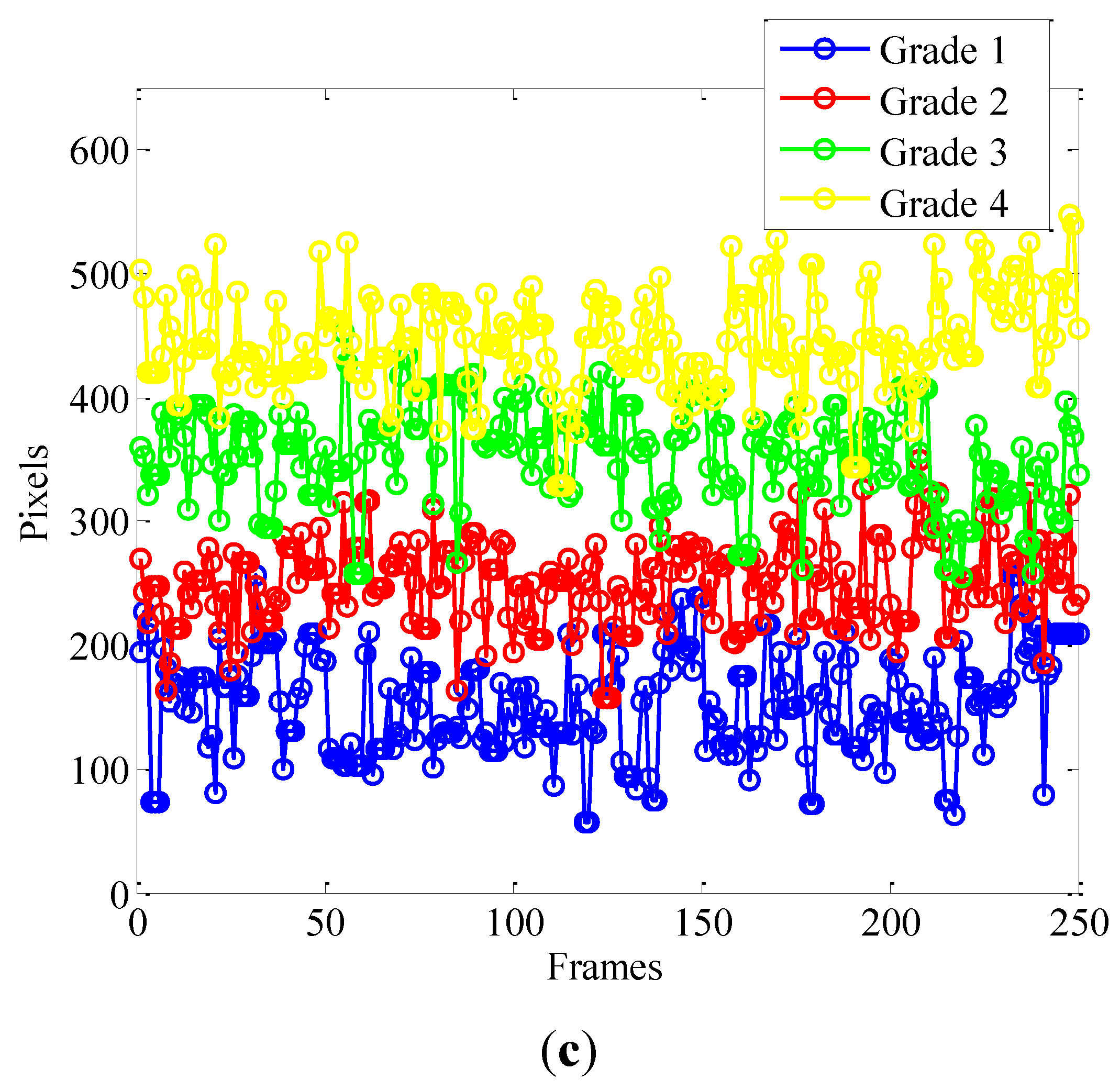
Distribution curves of white spot pixels in 10 s (250 frames for each grade) at different RH are shown in
Figure 11. Pixel numbers of insulators with high contamination grades are higher than that of insulators with low contamination grades. As is shown in
Figure 11, UV images have abilities to characterize the differences of discharge intensities between each grade.
Figure 11.
Distribution curves of white spot pixels in UV images. (a) RH = 80%; (b) RH = 85%; (c) RH = 90%.
Figure 11.
Distribution curves of white spot pixels in UV images. (a) RH = 80%; (b) RH = 85%; (c) RH = 90%.
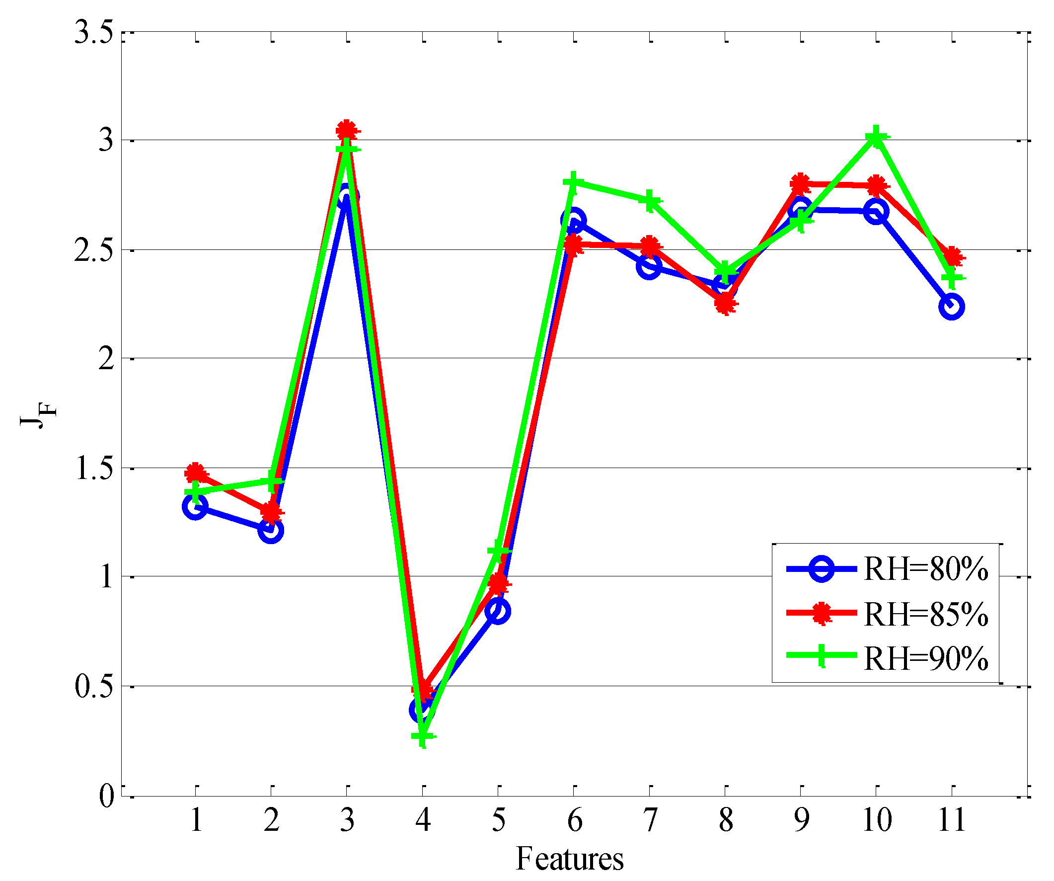
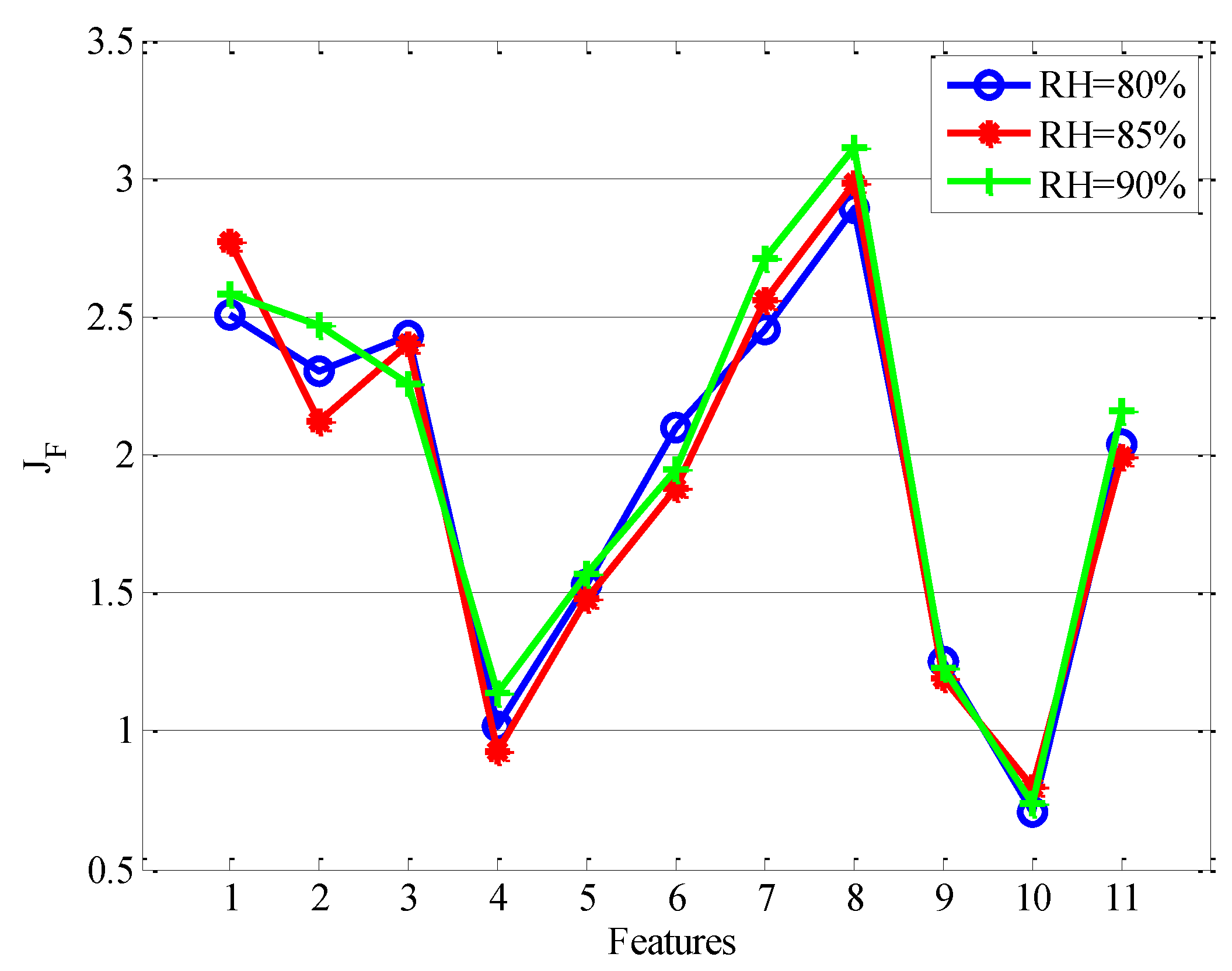
2.5. Feature Selection Based on Fisher Criterion
As mentioned above, feature sets of IR and UV images can be obtained after preprocessing and feature calculation. However, only a part of information is useful for the identification of contamination grades. Moreover, the irrelevant information degrades the recognition accuracy and increases the computing complexity. Therefore, selecting a subset of features containing the discriminative information is very important for the contamination grades recognition. In our research, Fisher criterion was applied to select powerful features from initial feature sets. Ratio of inter-class variance to intra-class variance is the evaluating indicator of Fisher criterion [
24].
Supposing the number of samples in data set is
n. The samples belong to different classes, which are given as ω
1, ω
2, …, ω
C, where
C is the number of classes (in this paper, it is four). The number of samples in each class is given as
ni,
i=1, 2, 3, 4.
is the inter-class variance of feature
k. And
is the intra-class variance of feature
k.
k is the dimension (feature number) of sample
x. Formulas of
and
are given as:
where
is the value of feature
k in sample
x,
is the mean value of feature
k in class
i,
is the overall mean of feature
k. Discriminant function of Fisher criterion is given as:
JF(k) is the criterion of feature k. Value of JF represents the differential degree of the feature. Generally speaking, if the JF of a feature is larger than two, this feature has sufficient capacity for differentiating.
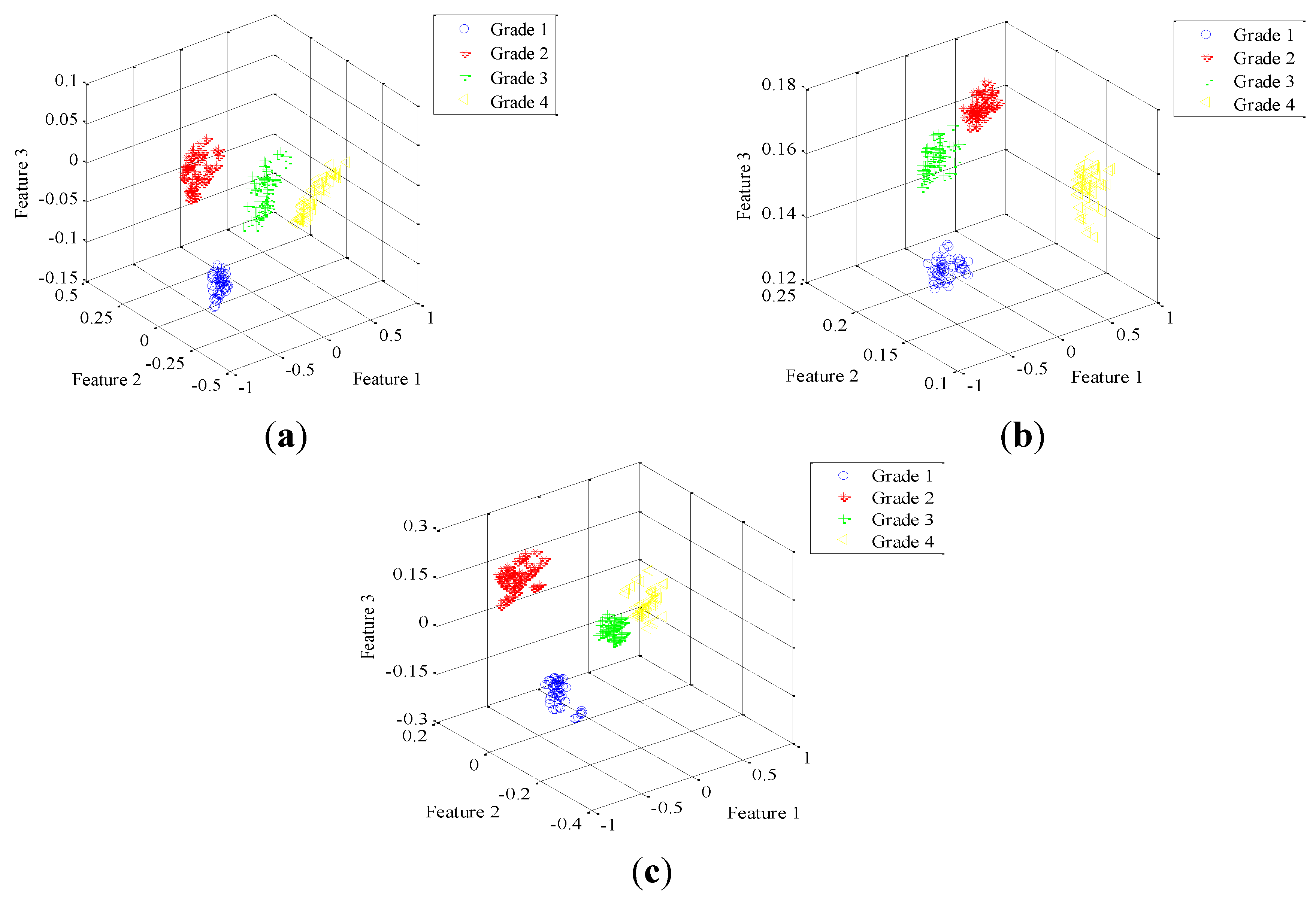
2.6. Feature Fusion Based on Kernel Principal Component Analysis (KPCA)
The serial combination of two types of selected features is the ordinary feature level fusion method. However, high dimensionality and redundancy of the combined feature increase the computing time of classifier and decrease the accuracy of recognition. KPCA has strong capability of dimension reduction and redundancy elimination. Fused features with strong classification ability can be extracted from the combined features by the utilizing of KPCA [
25]. Meanwhile, because of the dimension reduction, computational burdens of subsequent recognition can be eased significantly. On the basis of above analysis, KPCA was adopted to realize the fusion of IR and UV selected features in our research.
In KPCA, input data are transformed into a higher dimensional linear feature space by kernel function mapping. And then, principal component analysis (PCA) is adopted to process the mapping data in high-dimensional feature space and extract principal components, which can represent the characteristics of different contamination grades. Because of the capability of non-linear feature extraction, KPCA can extract the feature set which is more suitable in categorization than conventional PCA.
Supposing
is the original feature matrix, where
k = 1, 2, 3,
…,
N,
M is the dimension of feature set,
N is the number of samples. Original feature space
R is mapped onto high-dimensional feature space
F by nonlinear mapping φ. Supposing the mapping data is zero-mean, the covariance matrix of mapping data is given as [
26]:
After the eigenvector analysis of
C, we can derive that
.
i is the number of eigenvalues and eigenvectors. It can be derived from Equation (19) that:
where
After putting Equation (21) into Equation (20), a new expression of Equation (20) is given as:
Defining
K as kernel matrix, where
When both sides of Equation (22) are multiplied by φ(
xl)
T, it can be seen that:
Equation (24) can be expressed as
. The simplified formula is:
where α
i is a
N-dimensional column vector composed by α
ni. Kernel principal component can be calculated as:
Above equations are derived under the hypothesis that the mapping data have the characteristic of zero-mean. Generally speaking, this hypothesis is untenable in practice. Therefore, the mapping data need to be centralized. In order to realize the centralization,
K in Equation (25) is substituted by
, where
IN is a
N ×
N matrix with element of 1/
N. Inner product operation needs to be carried out in the process of extracting nonlinear principal component. In order to simplify the calculation, inner product operation is substituted by kernel function. Compared with other kernel functions, classifying quality of radial basis function (RBF) is the best. Formula of RBF is:
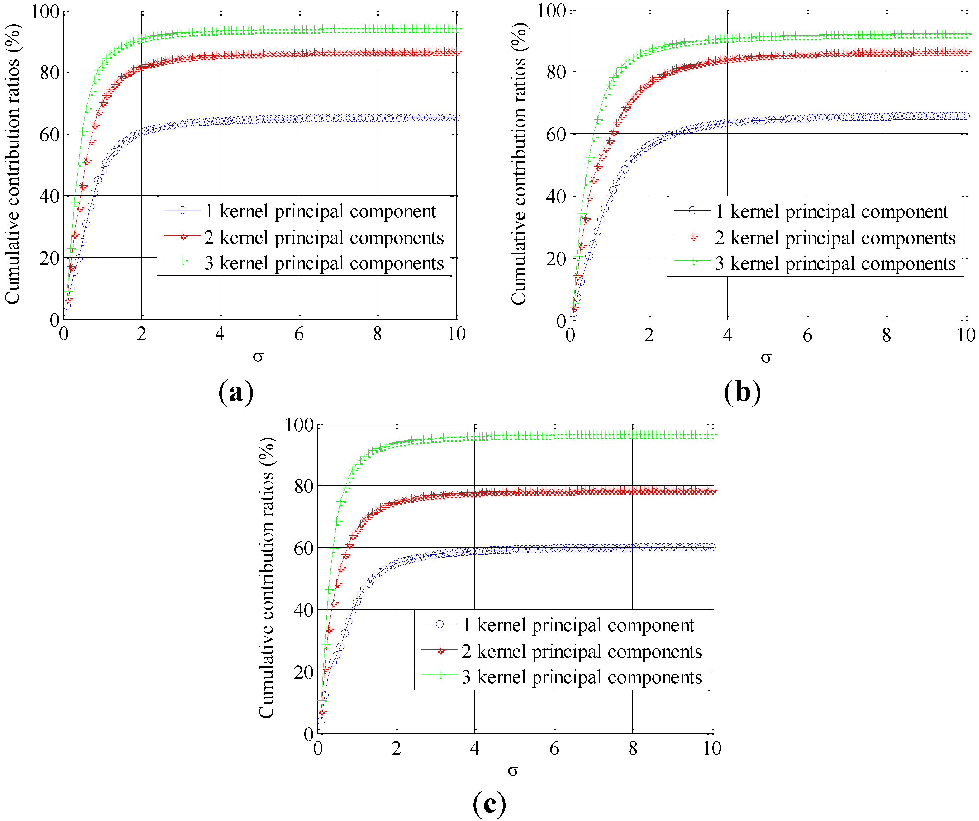
where σ is the width parameter of RBF. Cumulative contribution ratio γ
k is the evaluation index of kernel principal component selection. Kernel principal component contribution ratio ρ
i and cumulative contribution ratio γ
k are given as [
27]:
k is the number of selected kernel principal components.
N is the total number of kernel principal components, which equals to the number of analyzed samples. The importance of selected kernel principal components is reflected by ρ
i and γ
k. When γ
k is equal to or greater than 90%, the selected kernel principal components contain the main information of original data matrix and are suitable for subsequent classification.
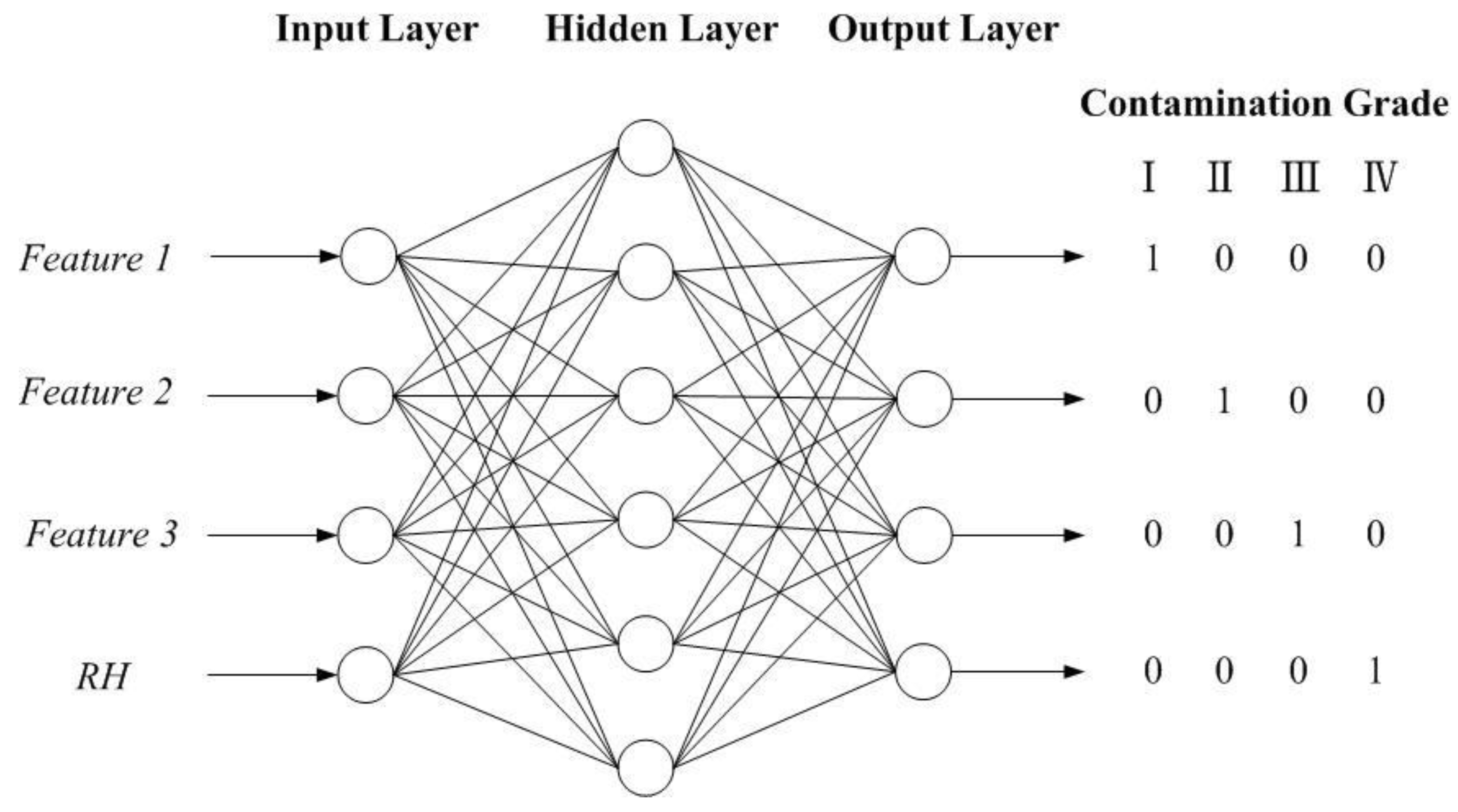
2.7. PSO-BPNN Classifier
Constructing an effective classifier is of great importance in this study. Artificial neural network (ANN), which has a high degree of self-learning, self-organization and adaptive capacity, can be used in many problems, such as modeling, pattern recognition and prediction, etc. Back propagation neural network (BPNN) classifier was applied to the recognition of contamination grades in this paper. Neural network input includes the fused features and corresponding RH. Neural network output is contamination grade. Because BPNN is easy to fall into local optimum, the global optimal solution is difficult to be guaranteed in training process. Meanwhile, problems, such as slow convergence speed and low accuracy, also restrict the application effect of BPNN. In order to overcome these disadvantages, particle swarm optimization (PSO) was used to optimize the training process of BPNN.
PSO is a kind of bionic optimization algorithm based on the imitation of bird foraging behavior. Every particle has three parameters: Position, velocity and fitness function. Position is a possible optimal solution for the optimization problem (in this study, the optimization problem is the adjustment of weights and thresholds of network neurons). Particle velocity (including direction and value) is dynamically adjusted towards local optimum and global optimum in light of experiences of the individual and the group. Fitness function value is calculated by objective function of optimization. In iteration, position and velocity of a particle are updated on the basis of individual extreme (a position with the minimum fitness value that a certain particle has ever experienced) and group extreme (position of a particle, which has the minimum fitness value in whole swarm). Individual extreme is the optimum position experienced by an individual particle. Group extreme is the global optimum position found by all particles. Positions and velocities are adjusted based on individual extreme and group extreme at each step of iteration. Meanwhile, individual extreme and group extreme are also updated according to the fitness function value. After certain steps of iteration, a particle with best fitness is taken as the optimal solution of optimization problem. Compared with other optimization algorithms, PSO has lower complexity and fewer parameters to regulate.
Supposing there are
m particles in a swarm, position vector of particle
i is
(in this study, position vector is composed of weights and thresholds of neurons), velocity vector is
,
n is the total number of optimized parameters. According to fitness function, fitness value of every position can be calculated.
is defined as the individual extreme,
is defined as the group extreme of whole swarm. At each step of iteration, velocity and position of a particle are updated in accordance with Equations (31) and (32).
where
i is the particle number,
j is the parameter number,
c1 and
c2 are learning factors,
r1 and
r2 are random numbers at the range of [0,1], ω is inertia weight. Inertia weight is dynamically adjusted as follows:
where ω
max is initial inertia weight, ω
min is the inertia weight at the end of iterative process,
t is the number of current iteration,
tmax is the maximum number of iteration. Mean square error (MSE) of BPNN outputs is selected as the fitness function. Computational formula of MSE is:
where
P is the number of training samples,
s is the number of output neurons,
u represents the actual output of BPNN,
y represents the desired output of BPNN. The first part of Equation (31) represents influence of current velocity to next iteration; the second part represents the influence of individual extreme (individual experience); the third part represents the influence of group extreme (group experience). In training process of PSO-BPNN, weights and thresholds of neurons are adjusted in accordance with PSO principle mentioned above.


