Stable Operation and Electricity Generating Characteristics of a Single-Cylinder Free Piston Engine Linear Generator: Simulation and Experiments

Abstract

We present a novel design of a single-cylinder free piston engine linear generator (FPELG) incorporating a linear motor as a rebound device. A systematic simulation model of this FPELG system was built containing a kinematic and dynamic model of the piston and mover, a magneto-electric model of the linear generator, a thermodynamic model of the single-cylinder engine, and a friction model between the piston ring and cylinder liner. Simulations were performed to understand the relationships between pre-set motor parameters and the running performance of the FPELG. From the simulation results, it was found that a motor rebound force with a parabolic profile had clear advantages over a force with a triangular profile, such as a higher running frequency and peak cylinder pressure, faster piston motion, etc. The rebound position and the amplitude of rebound force were also determined by simulations. The energy conversion characteristics of the generator were obtained from our FPELG test rig. The parameters of intake pressure, motor frequency, and load resistance were varied over certain ranges, and relationships among these three parameters were obtained. The electricity-generating characteristic parameters include output power and system efficiency, which can measure the quality of matching the controllable parameters. The output power can reach 25.9 W and the system efficiency can reach 13.7%. The results in terms of matching parameters and electricity-generating characteristics should be useful to future research in adapting these engines to various operating modes.

1. Introduction

Recently, energy conservation pressures and environmental protection demands for high fuel efficiency have led to an increasing interest in unconventional engine configurations within academia and industry [1]. All devices that consume energy and pollute the environment are of importance; the internal combustion engine is one such device. The number of modern vehicles powered by internal combustion engines, except for some electric vehicles, is increasing world-wide. Concurrently, the Earth’s sources of crude oil are decreasing. Moreover, increasingly stringent emissions standards force automobile suppliers into a never-ending effort to design, manufacture, and market less-polluting and more fuel-efficient vehicles [2]. Therefore, free piston engine generators have been a subject of research and development in new power devices in recent years because of their special and simple configuration. The free piston engine linear generator (FPELG) is an internal combustion engine and linear generator coupled system. Compared with a traditional internal combustion engine, an FPELG has many potential advantages [3,4,5], including higher partial-load efficiency and multi-fuel possibilities because of its flexibility to optimize combustion, reduced weight from fewer engine components, and reduced heat-transfer losses and NO_x emissions due to a faster power stroke expansion capability [1,2,3,4]. Therefore an FPELG can be used in electric vehicles with potential advantages such as energy savings, environmental friendliness, and high power density [3,6,7].

The free-piston engine concept was first introduced in the 1920s by Pescara [8], who patented the engine as an air compressor. Since then, many companies worldwide have designed and developed free-piston engines, such as SIGMA in France, Junkers [9] in Germany, General Motors, Ford Motor Company, etc. Most prototypes were used as air compressors or gas generators. The development of these engines was abandoned until the 1960s because free-piston engine technology was viewed as not commercially viable [3]. Recently, free-piston engine concepts have again stimulated interest among research groups due to the appearance of many burgeoning technologies. Sandia National Laboratory presented the design of a dual piston free-piston engine generator with homogeneous charge compression ignition (HCCI) whose electrical power output was 40 kW. The experiments demonstrated a thermal efficiency of 56% with low emissions [10]. Steady operation had been realized based on precise motion control in work at Czech Technical University. When a prototype was running with a frequency of 27 Hz and a compression ratio of 9, the average power output was approximately 650 W [11]. Mikalsen and Roskilly studied the design and simulation of a single-cylinder free-piston engine generator with a gas-filled bounce chamber, and discussed the influences of some parameters on the system’s performance over a wide operating range [12]. Some researchers study the piston motion control strategies of the FPELG because effective engine control is the main prerequisite for this novel system to be feasible and applicable [4,6,7,8,9,10,11,12,13,14,15]. The fundamental characteristics and control system of prototype of single-cylinder two-stroke FPELG were investigated by Kosaka et al. [15] and Goto et al. [16], respectively. The operation frequency was 23 Hz. The researchers also analyzed and assessed two cases of spark ignition and premixed charge compression ignition combustion [14,17]. FPELG is a crankless linear dynamic system [18]. It has unique features compared with other power system such as being highly integrated with engine and generator, high power density, small friction loss, high thermal efficiency, low vibration and radiated noise, good fuel adaptability, difficulty for steady running, etc. The electricity generating characteristics are a part of the load characteristics for a FPELG. However, a piston motion control system is hard to realize because of the absence of a crankshaft, though this enables possibly extensive possibilities for optimization of engine operation [19,20,21,22]. The single-cylinder FPELG designed in this article has a simple configuration with high controllability for its application to the rebound device, which is compact. Although this structure has the essential feature of variable compression ratio, the prototype is easy to operate stably by controlling the linear motor. In this condition, the combustion heat release and electricity generating characteristics, energy conversion relations can be studied in experiment. The linear motor can also be used as an auto starting device and energy compensating device. These benefits can promote its production and commercialization.

Firstly, the rebound linear motor should be adapted. The motor provides the rebound force when the piston reaches to BDC. Since it can be controlled, the profile and value of rebound force will be confirmed by simulation. As the control program affects operating performance and generating characteristics, we firstly model the motor rebound force pattern and the rebound position by way of simulation. Then, we use a gas intake system to replace the cylinder of the prototype. The gas intake pressure is the indicator of energy input, which is varied in experiments. The load resistance is the indicator of load and consumption of the system, and the frequency is the indicator of motion features. Finally, the output power and system efficiency are used as the electricity generating indicator to measure the quality of how appropriately the controllable parameters are matched. Our goal is to characterise the load coupling under various conditions and the transitions between modes of operation.

2. Simulation Modelling and Methodology

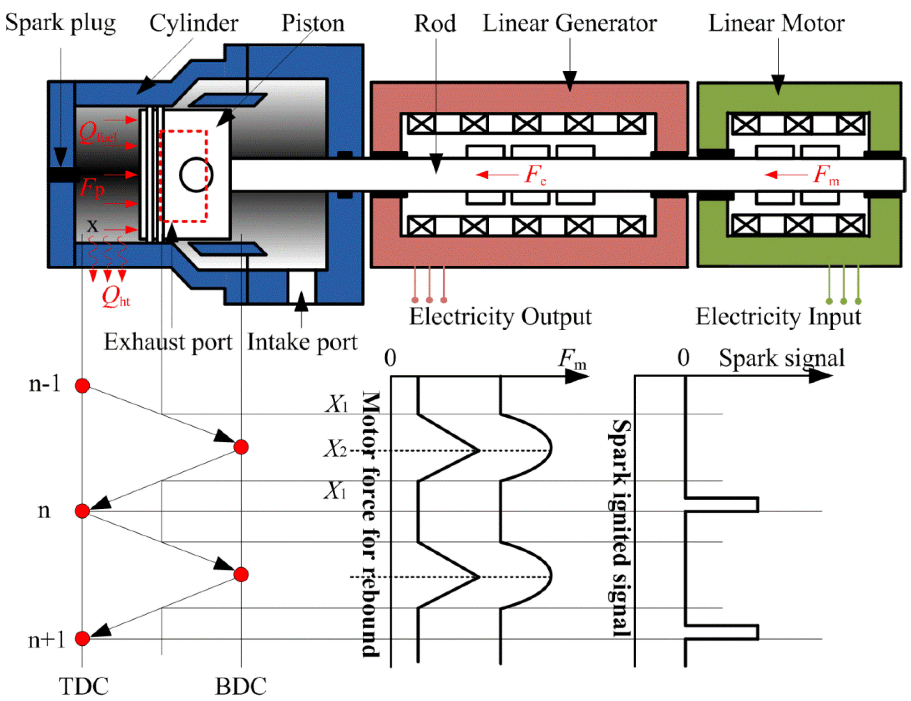
2.1. Linear Motor Force Profiles

The single-cylinder FPELG under study consists of four main modules: combustion cylinder, piston, linear generator, and linear motor, as shown in Figure 1. The linear generator is a load device, while the linear motor is the rebound device that creates rebound forces following certain pre-defined programs. The combustion cylinder does not have intake and exhaust valves, but rather air inlet and exhaust ports, which are set on opposite sides of the cylinder to enable port scavenging. The piston is rigidly connected to the rod of the linear generator and linear motor. Permanent magnets are attached to specific positions along the rod. These define the secondary units of the linear generator. Coils are set in the generator. When the piston reciprocates, the magnetic fields of the permanent magnets move through the coils to induce electromagnetic force. The piston moves from TDC to BDC in the power stroke. Because there is only one cylinder in the system, the piston could not return from BDC without the linear motor. The motor is the key module of the system because it bounces the piston and also can control its motion. The linear motor is the primary difference between traditional types of single-cylinder free-piston engines and the FPELG of this paper.

The FPELG runs stably when the piston moves continuously between TDC and BDC. Figure 1 also illustrates the running sequence of this system. Continuous cycles are indicated by n − 1, n and n + 1. The changes of signals are also indicated with the corresponding piston positions. When the piston position is larger than X₁ (shown in Figure 1), the force generated by the motor will reach a value sufficient to decelerate the piston in the power stroke before it reaches BDC and to drive the piston backward in the compression stroke of the next cycle before it reaches TDC. The rebound position and the value of motor force completely determine the length of the stroke and frequency of the system. Hysteretic rebound position or smaller motor rebound force results in a longer stroke and lower frequency of motion. The linear motor can recover some energy by slowing down the piston by acting as a brake, so that the piston can be controlled by the motor force. In the design of the prototype, alternative timing positions were implemented to obtain different motion profiles through different levels of motor force.

Figure 1. Configuration of a single-cylinder FPELG.

Figure 1. Configuration of a single-cylinder FPELG.

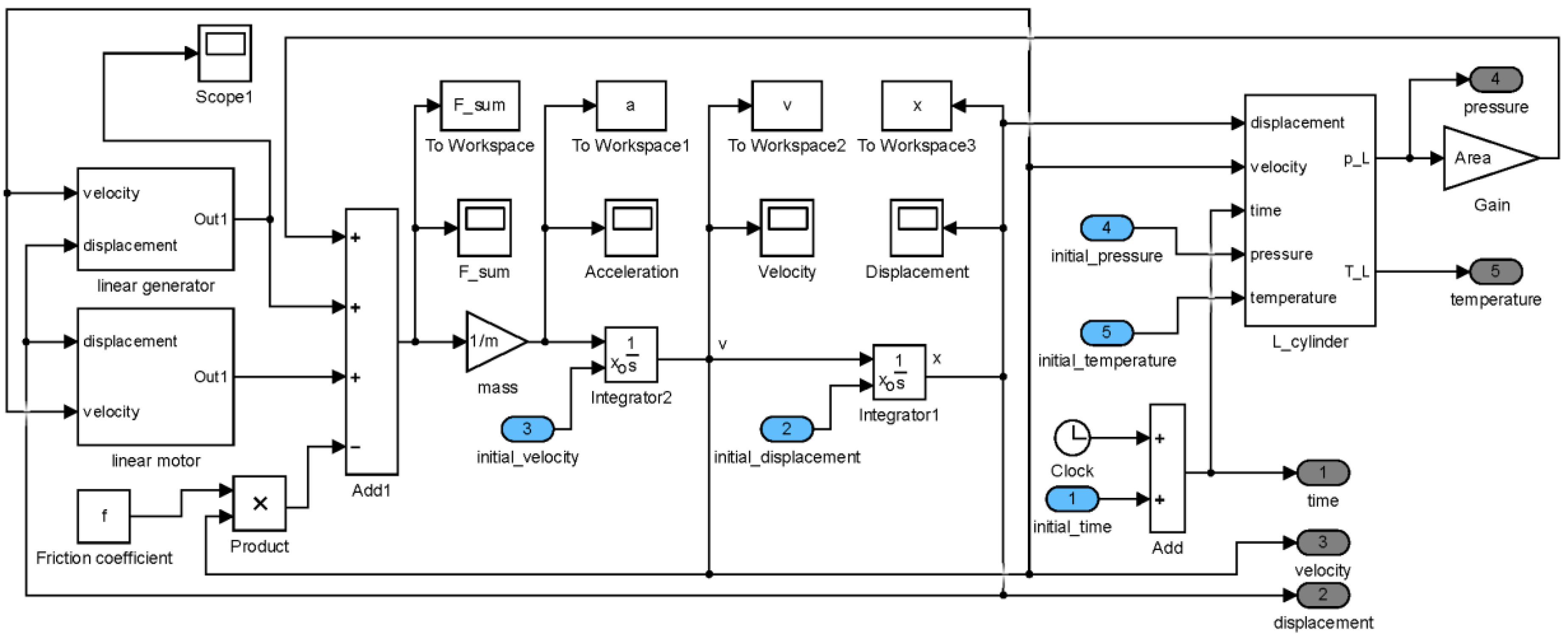
2.2. Simulation Model

2.2.1. Dynamic Modeling

In the FPELG, the motion of the piston assembly at any point in the cycle is determined by the sum of the forces acting on it. These forces are the combustion chamber pressure force F_p, the motor force F_m, the frictional force F_f, and the electromagnetic force F_e. Let x denote the position of the moving part, t the time and m the mass of the piston assembly. The system obeys Newton’s Second Law, and the piston motion can be described by:

$$m\frac{{\text{d}}^{2}x}{\text{d}{t}^2}=F_{\text{p}}+F_{\text{f}}+F_{\text{e}}+F_{\text{m}}$$

(1)

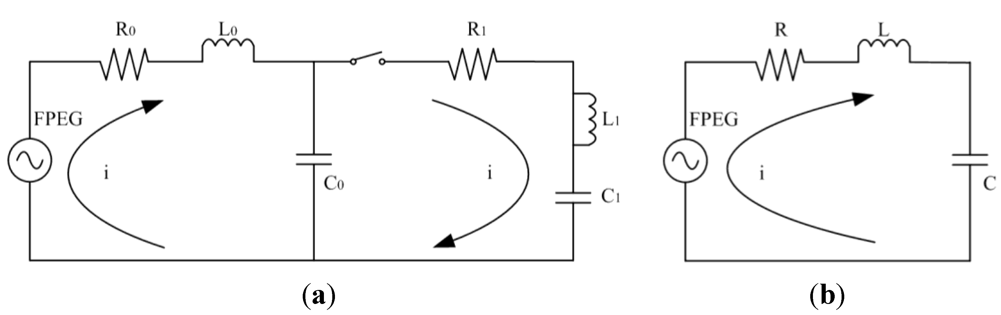
2.2.2. Linear Generator Modeling

A commercial permanent-magnet linear generator was chosen to minimize design cost and time in the prototype [2]. The operation of the linear generator is periodic during operation of the FPELG. The velocity of the piston through the generator fluctuates from zero to maximum and then back to zero. Thus the generator is always in a dynamic process [18,23].

Generally, most generators can be described by an equivalent circuit diagram as shown in Figure 2a. The two loops represent the engine and load loops. This can be simplified to the RLC circuit in Figure 2b.

Figure 2. (a) FPELG equivalent circuit diagram; (b) Simplified FPELG equivalent circuit diagram.

Figure 2. (a) FPELG equivalent circuit diagram; (b) Simplified FPELG equivalent circuit diagram.

The voltage equation for this linear generator can be written as:

$$R\cdot i+L\cdot \frac{\text{d}i}{\text{d}t}+V_{\text{c}}=e_{\text{g}}$$

(2)

From the Faraday Electromagnetic Law:

$$e_{\text{g}}=-\frac{\text{d}\Phi }{\text{d}t}$$

(3)

Assuming that the flux linkage is a function of x, then:

$$e_{\text{g}}=-\frac{\text{d}\Phi }{\text{d}t}=-\frac{\partial \Phi }{\partial x}\cdot \frac{\text{d}x}{\text{d}t}=-k_{\text{g}}\cdot \dot{x}$$

(4)

where k_g is determined by the structure of the generator. Ignoring dissipation in the system, from power conservation we obtain Equation (5) as follows:

$$F_{\text{e}}\cdot \dot{x}=e_{\text{g}}\cdot i$$

(5)

The following can be derived from Equations (4) and (5):

$$F_{\text{e}}=-k_{\text{g}}\cdot i$$

(6)

Furthermore, if the voltage and current are the same, namely the inductance and the capacitance are counteractive, Equation (2) can be written as:

$$i=e_{\text{g}}/R$$

(7)

From Equations (4) and (5), we obtain Equation (8) as:

$$F_{\text{e}}=\frac{k_{\text{g}}^2}{R}\cdot \dot{x}=c\cdot \dot{x}$$

(8)

That is, the electromagnetic force F_e is proportional to the velocity, and c is a constant of the load.

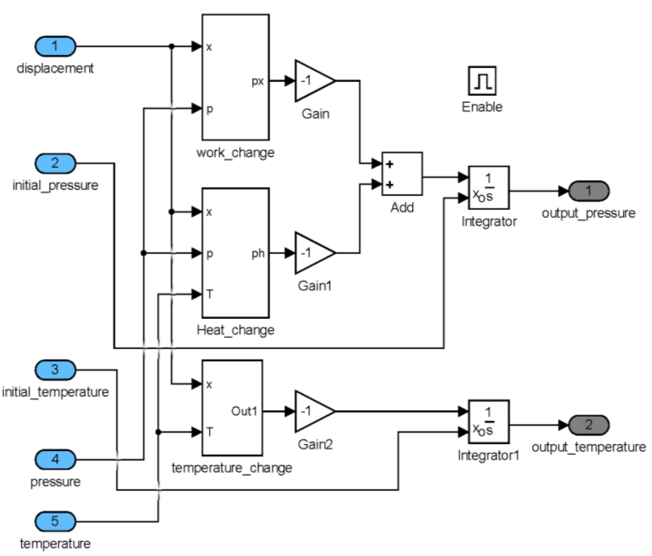
2.2.3. Thermodynamic Modelling

The thermodynamic analysis of the FPELG is based on the first law of thermodynamics and equation of state of an ideal gas. The entire system can be seen as an open system. Assuming that at any instant in time the temperature and pressure in the cylinder are in thermodynamic equilibrium, and ignoring the effects of vaporizing liquid droplets, fluid flow, combustion chamber geometry or spatial variations of the mixture’s composition, the equations describing the state in the cylinder are the conservation of mass and the first law of thermodynamics [2,4,5,24]:

$$\frac{\text{d}U}{\text{d}t}=-P\frac{\text{d}V}{\text{d}t}+\frac{\text{d}Q}{\text{d}t}+{\displaystyle \sum H_i}$$

(9)

where ${\displaystyle \sum H_i}={\dot{H}}_i-{\dot{H}}_e$, ${\dot{H}}_i$ and ${\dot{H}}_e$ are the enthalpy output and input, and Q is the energy input:

$$\frac{\text{d}Q}{\text{d}t}=\frac{V}{\text{γ}-1}\frac{\text{d}p}{\text{d}t}+p\frac{\text{γ}}{\text{γ}-1}\frac{\text{d}V}{\text{d}t}$$

(10)

Considering $\frac{\text{d}Q}{\text{d}t}=\frac{\text{d}{Q}_{\text{c}}}{\text{d}t}-\frac{\text{d}{Q}_{\text{h}}}{\text{d}t}$, then Equation (10) can be written as:

$$\frac{\text{d}p}{\text{d}t}=-\text{γ}\frac{p}{V}\frac{\text{d}V}{\text{d}t}+\frac{\text{γ}-1}{V}(\frac{\text{d}{Q}_c}{\text{d}t}-\frac{\text{d}{Q}_{ht}}{\text{d}t})$$

(11)

The in-cylinder heat transfer effect is modelled according to Hohenberg [19]:

$$\frac{\partial Q_{\text{ht}}}{\partial t}=hA(T-T_{\text{w}})$$

(12)

The heat transfer coefficient h is given by:

$$h=130V^{-0.06}{(\frac{p}{{10}^5})}^{0.8}{T}^{-0.4}{(\overline{U}+1.4)}^{0.8}$$

(13)

where Tw is the temperature of the cylinder wall, $\overline{U}$ is the mean piston speed, p is the in-cylinder pressure, and T is the temperature of the gas in the cylinder.

Because the engine has no crankshaft, a time-based Wiebe function (as opposed to a conventional crank-angle based approach) is used to express the mass fraction burned in the combustion model as [5,18]:

$$x(t)=\frac{m_{\text{b}}}{m}=1-\exp \left[-a{(\frac{t-t_0}{t_{\text{c}}})}^{1+b}\right]$$

(14)

$$\frac{\text{d}{Q}_{\text{c}}}{\text{d}t}=Q_{\text{in}}\frac{\text{d}x(t)}{\text{d}t}$$

(15)

where m is the injected fuel mass, x(t) is the fuel mass fraction burned, m_b is the burned fuel mass, a and b are shaping factors, t₀ is the time when combustion begins, t_c is the combustion duration and Q_in is the overall heat input.

2.2.4. Frictional Modelling

Because the FPELG does not have a crankshaft and connecting rod mechanism, there is no piston side thrust, and friction is greatly reduced. To simplify the calculation, friction is taken as a constant. The value for the friction force is determined using a correlated empirical equation of the piston ring and piston friction. The mean frictional pressure for two-stroke engines is given as follows [20]:

$$f_{\text{mep}}=A\cdot S\cdot n=\frac{W_{\text{f}}}{V_{\text{d}}}$$

(16)

where A = 150 kg·m⁻²·s⁻¹, S is the maximum stroke length, n is the oscillating frequency of the piston, W_f is the work required to overcome friction and V_d is the displaced volume:

$$V_{\text{d}}=\frac{\text{π}{D}^{2}S}{4}$$

(17)

$$W_{\text{f}}=F_{\text{f}}\cdot 2S$$

(18)

where D is the bore of the cylinder. Substituting Equations (17) and (18) into Equation (16), we have:

$$F_{\text{f}}=\frac{\text{π}{D}^2{f}_{\text{mep}}}{8}$$

(19)

2.3. Simulation Method

There are various parameters in the mathematical model, and some of the key model parameters and simulation parameters for this single-cylinder FPELG are listed in Table 1 and Table 2. They are applied in the numerical simulation to show the results of this design.

Table 1. Parts of key parameters of the single-piston engine generator.

Parameters	Value
Bore	34.0 mm
Piston assembly mass	5.0 kg
Spark ignited position	3.0 mm
Intake port open position	28.0 mm
Exhaust port open position	25.0 mm
Initial pressure in cylinder	1.013 × 105 Pa
Load constant	100 Ns/m
Design stroke	45 mm

Table 1. Parts of key parameters of the single-piston engine generator.

Parameters	Value
Bore	34.0 mm
Piston assembly mass	5.0 kg
Spark ignited position	3.0 mm
Intake port open position	28.0 mm
Exhaust port open position	25.0 mm
Initial pressure in cylinder	1.013 × 105 Pa
Load constant	100 Ns/m
Design stroke	45 mm

Table 2. Parts of simulation parameters of the single-piston engine generator.

Parameters	Value
Combustion duration	4.5 ms
Combustion quality factor	2
Average velocity y of piston	3 m/s
Specific heat ratio in compression stroke	1.33
Specific heat ratio in expansion stroke	1.30
Lower heating value of fuel	4.4 × 107 J/kg

Table 2. Parts of simulation parameters of the single-piston engine generator.

Parameters	Value
Combustion duration	4.5 ms
Combustion quality factor	2
Average velocity y of piston	3 m/s
Specific heat ratio in compression stroke	1.33
Specific heat ratio in expansion stroke	1.30
Lower heating value of fuel	4.4 × 107 J/kg

Figure 3 presents the Simulink dynamic block model for the simulation. In the diagram, the block “engine” that transfers the parameters x, v, t to F_p is expanded in Figure 4. This diagram contains the “stateflow” module. It is used to indicate the logic relationships of all of the system operation conditions such as the combustion process, the scavenge process, the rebound process, etc. The simulation time step was set to 10⁻⁵·s [16].

Figure 3. Simulink diagram for the simulation.

Figure 3. Simulink diagram for the simulation.

Figure 4. Block diagram of the “engine” subsystem.

Figure 4. Block diagram of the “engine” subsystem.

2.4. Simulation Results and Discussion

In the simulation model, the rebound position and value of motor force were set in series. This is because different motor forces and different rebound positions can influence the combustion performance in cylinder. Additionally, the motor rebound force pattern should be confirmed to attain high combustion efficiency.

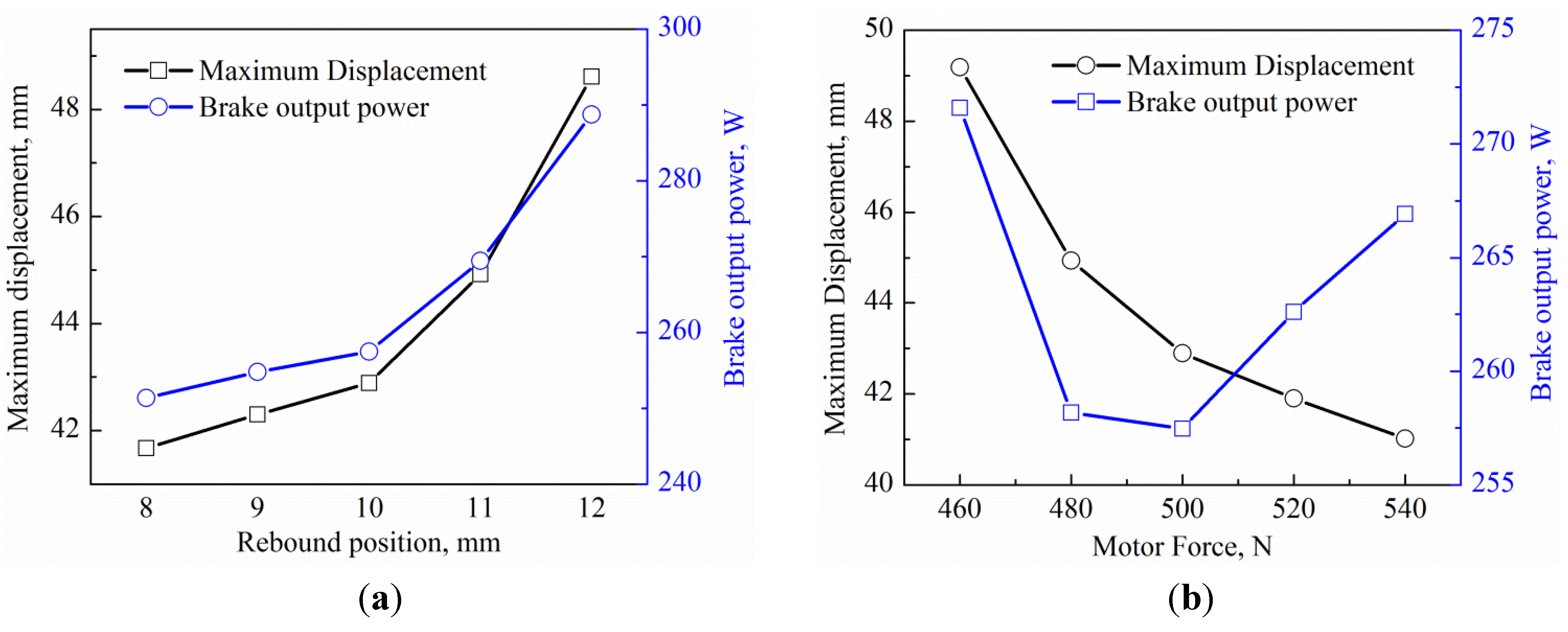
2.4.1. Different Motor rebound Forces and Positions

The motor force can be controlled, so it can be therefore changed to obtain different results. In Figure 5a, the curves reflect the maximum displacements and braking output powers with motor forces of 460 N, 480 N, 500 N, 520 N, and 540 N. If the motor force is lower than 500 N, the capacity of constant volume combustion is better. Both conditions can keep brake output power higher.

Figure 5. (a) Maximum displacements and brake output power of the linear generator at different motor forces; (b) Maximum displacements and brake output power of the linear generator at different rebound positions.

Figure 5. (a) Maximum displacements and brake output power of the linear generator at different motor forces; (b) Maximum displacements and brake output power of the linear generator at different rebound positions.

Thus, both the motor force and the rebound position are important in this system. With decreasing motor force, the maximum displacement increases. That is, the lower rebound force requires more time to drive the piston back. Changing motor forces changes braking output power. The initial value at the 10 mm rebound position was 500 N, and with both an increase and decrease in the motor force, the brake output power of the linear generator increased. This is because the combustion process was influenced as a result of altering the motor rebound force. With the same rebound position, if the motor force is higher than 500 N, the combustion duration is shorter. Figure 5b shows the maximum displacements and brake output power at different rebound positions with the motor force of 500 N. When the rebound position increases, the maximum displacement and brake output power of the linear generator increase. Thus, the rebound position is vital for the system.

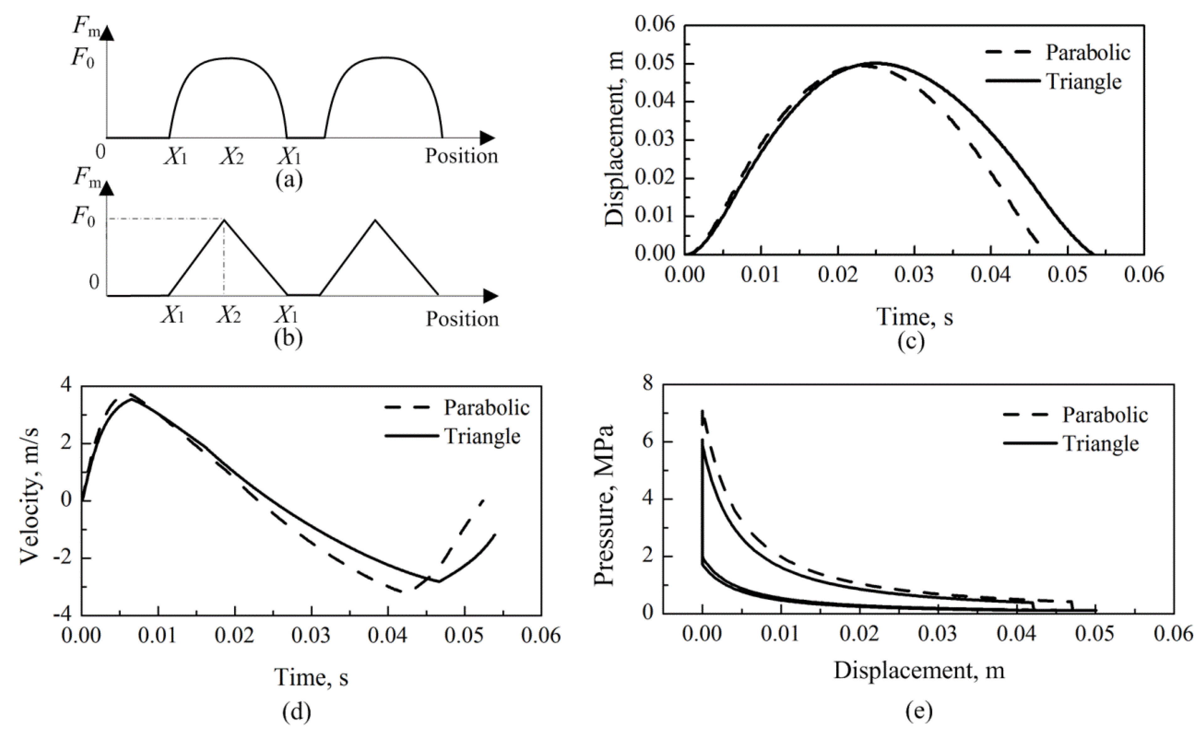
2.4.2. Different Motor Force Types

If the single free-piston engine operates in a particular stable state, the profile and value of motor force will be set with a particular rebound position. In this design, the profile of the motor force can vary with the set motor force and corresponding rebound position. The key principle of this single-cylinder FPELG is the energy conservation law. Figure 6a shows a parabolic motor force as the rebound force. For this force profile, X₁ is the start position, X₂ is the BDC position, and F₀ is the maximum value of its parabolic shape. Figure 6b shows the triangular profile motor force as the rebound force. Based on the law of conservation of energy, the work done by F_m is the same between X₁ and X₂. For the parabolic motor force, X₁ is 14 mm, X₂ is 47 mm, and F₀ is 800 N. For the triangular motor rebound force, X₁ is 15 mm, X₂ is 42 mm, and F₀ is 900 N. The results for these two situations are shown in Figure 6c–e.

Figure 6. (a) Parabolic profile of motor rebound force; (b) Triangular profile of motor rebound force; (c) Displacement of two motor rebound force profiles vs. time; (d) Velocity of two motor rebound force profiles vs. time; (e) Pressure of two motor rebound force profiles vs. displacement.

Figure 6. (a) Parabolic profile of motor rebound force; (b) Triangular profile of motor rebound force; (c) Displacement of two motor rebound force profiles vs. time; (d) Velocity of two motor rebound force profiles vs. time; (e) Pressure of two motor rebound force profiles vs. displacement.

Figure 6c shows displacement curves with differing motor rebound-force patterns. The various conditions under which the curves were recorded are identical. However, there are some differences in the dynamic results. The cycle duration with the parabolic motor rebound force is shorter than that of the triangular motor rebound force. The parabolic motor force reaches the TDC more quickly than the triangular motor force, with slight variations in maximum displacement. Figure 6d compares the velocities with different motor forces. The absolute values of the maximum positive and negative velocities with the parabolic motor force are higher than for the triangular motor force. The range and rate of change from positive to negative values is greater for the parabolic motor force. Thus, the range of variation is greater for the parabolic motor force. Figure 6e shows the cylinder pressure versus piston displacement for the two motor forces. The peak pressure is greater with the parabolic motor rebound force than with triangular motor force, and the time to reach the maximum pressure is shorter. Consequently, the compression stroke is shorter for the parabolic motor force. Additionally, the area under the parabolic force pressure curve is larger than that of the triangular force curve. This means the indicated output power is higher when the motor rebound force pattern is parabolic. Therefore the parabolic motor rebound force is more advantageous than the triangle motor rebound force, and this force pattern was set in the experiment.

3. Electricity Generating Characteristics of the Linear Generator

When our group used the free piston engine as energy input device, the system stability was poor since the piston movement was the result of the comprehensive action of different forces such as combustion gas pressure, electromagnetic resistance and linear motor force. However, as a disturbing factor, the electricity generating characteristics influenced the stable operation significantly. That was, the load resistance influenced the performance of the system significantly as an energy consumption device. Therefore, the experiment rig was transformed. To study the electricity generating characteristic under different load resistances, gas intake pressure and frequencies, the cylinder of engine was replaced by a gas intake cavity as shown in Figure 7.

Figure 7. FPELG configuration: ① Gas intake system; ② Gas intake cavity; ③ Load resistance; ④ Linear motor; ⑤ Linear alternator.

Figure 7. FPELG configuration: ① Gas intake system; ② Gas intake cavity; ③ Load resistance; ④ Linear motor; ⑤ Linear alternator.

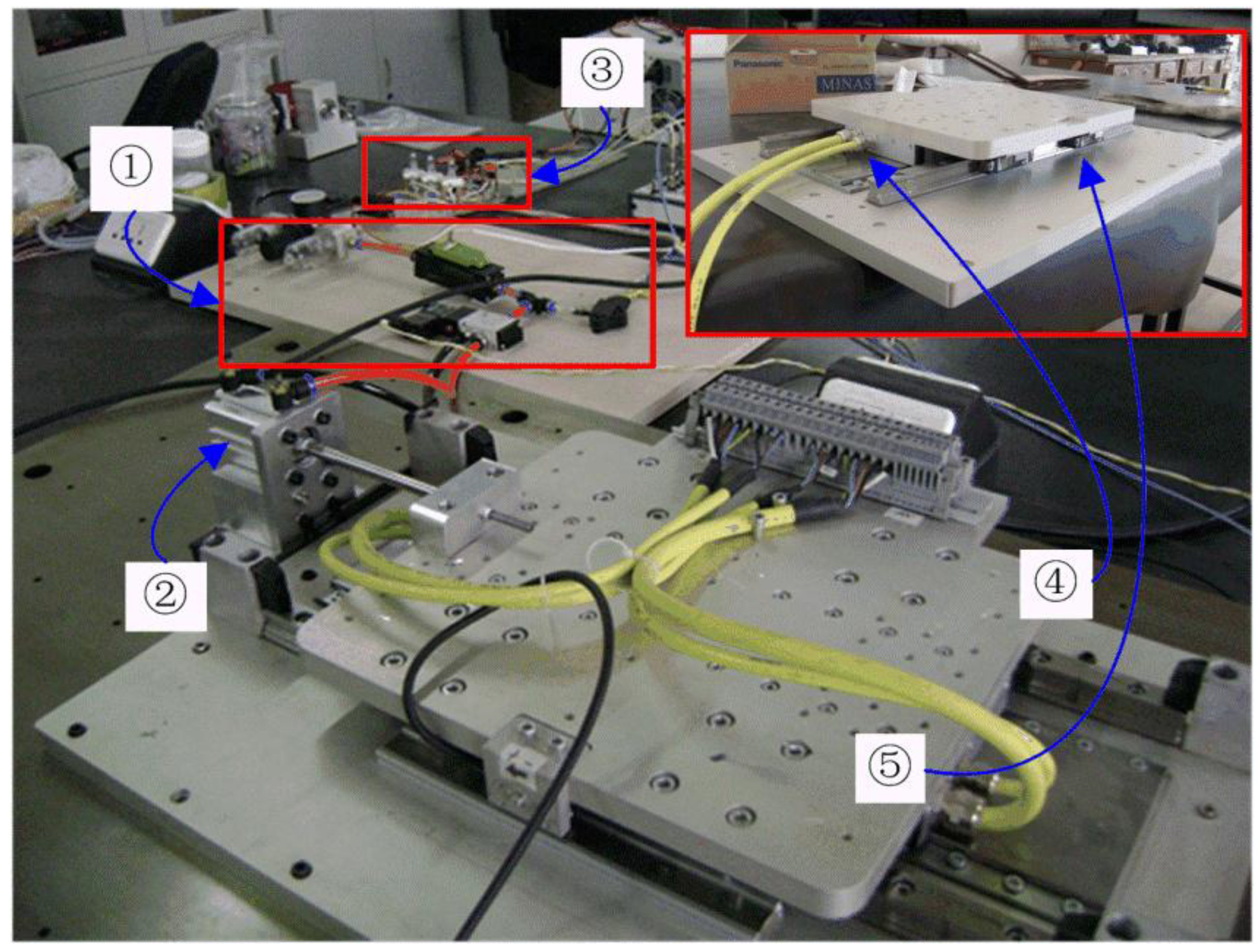
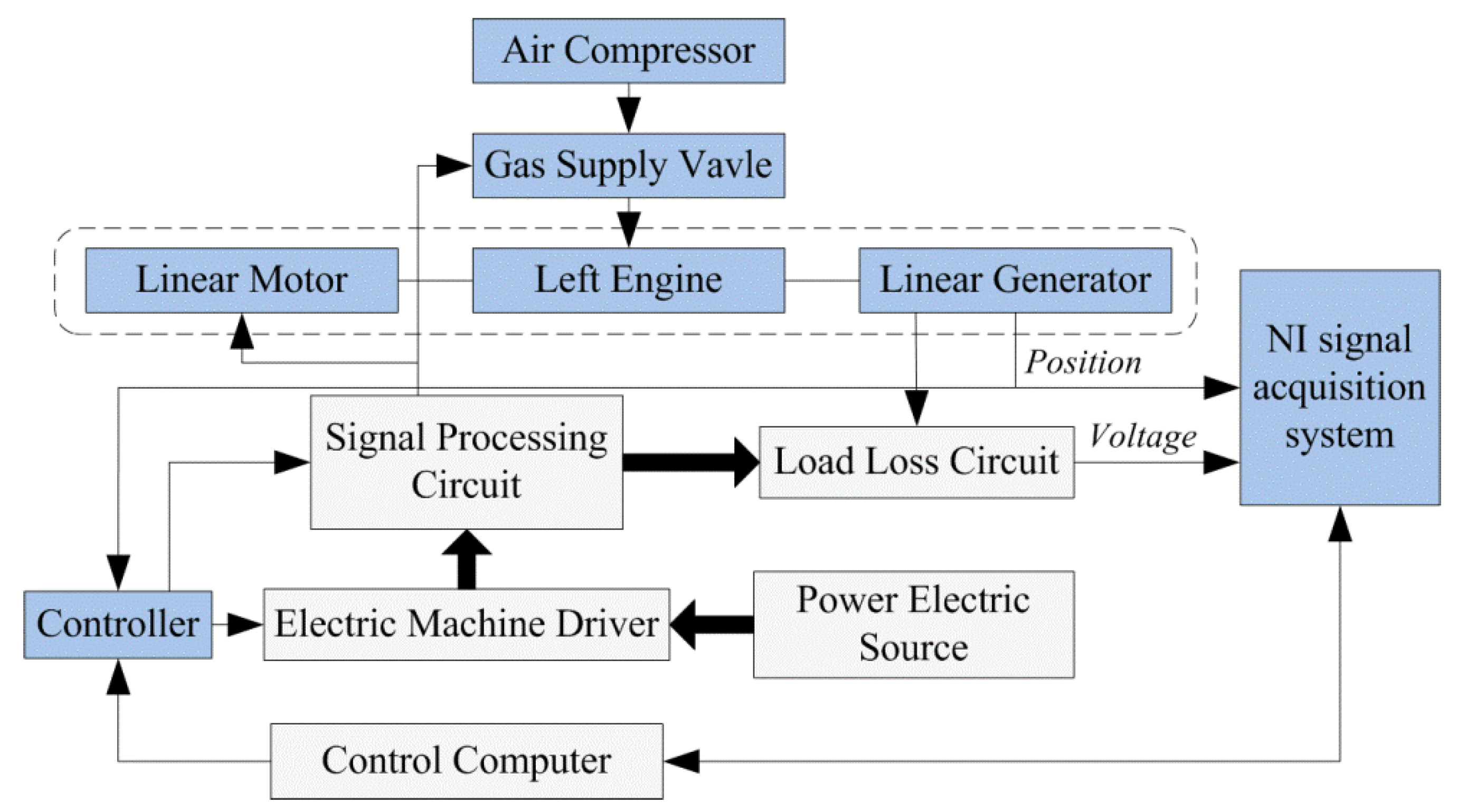
3.1. FPELG Prototype

Figure 7 is a photograph of the experiment rig. In addition to the prototype, the experimental test devices included the control and test systems. The control system was coupled to the driver and controller box of the linear motor, and the test system was coupled to the linear generator. The displacement signal was transformed from the encoder that fixed the linear generator to the driver, and we obtained it in a PC which was connected to the controller. When the system operated, there were two input powers. The gas pressure in the intake cavity acted on the mover. It rebounded back to compress the gas in the cavity under the force of the linear motor. The reciprocating motion of the mover produced the electricity power output of the linear alternator as the energy consumption.

Figure 8 shows the connection of the whole system. The major part was the single-cylinder FPELG prototype in the dashed frame. The left engine was replaced by a gas intake cavity. The air was supplied by the air compressor. The position signal used as feedback signal was from the encoder in the linear generator. It also could be gathered by a NI signal acquisition system. When the mover reached its set position on the left side, the gas supply valve was opened triggered by the signal from the processing system. The gas supply valve was an electromagnetic valve driven by the electrical machine driver. The linear motor was also controlled with the position feedback. When the mover reached the set position of the other side (BDC), the linear generator was started triggered by a signal from the controller. The control commands were edited in the control computer. All of the actions of the devices such as the gas supply valve and linear motor were driven by I/O commands.

Figure 8. The connection diagram of the system.

Figure 8. The connection diagram of the system.

Table 3. Parameters of the linear motor/generator.

Parameters	Linear Motor/Generator
Maximum stroke	180 mm
Actual stroke	50 mm
Width of air gap	7.2 mm
Width of the permanent magnet	12 mm
Turns per coil	180
Mass of permanent magnet	1.6 kg
Peak force	1300 N
Force constant (25 °C)	44.7 N/A
Continuous stall force	440 N
Peak current	41.5 A
Back EMF constant (ph-ph, °C)	25.8 V/(m·s−1)
Resistance	12 s
Peak velocity	19.2 m·s−1

Table 3. Parameters of the linear motor/generator.

Parameters	Linear Motor/Generator
Maximum stroke	180 mm
Actual stroke	50 mm
Width of air gap	7.2 mm
Width of the permanent magnet	12 mm
Turns per coil	180
Mass of permanent magnet	1.6 kg
Peak force	1300 N
Force constant (25 °C)	44.7 N/A
Continuous stall force	440 N
Peak current	41.5 A
Back EMF constant (ph-ph, °C)	25.8 V/(m·s−1)
Resistance	12 s
Peak velocity	19.2 m·s−1

Table 4. The test devices and their accuracy.

Test Device	Accuracy
Linear generator	0.01 mm
Electric machine controller	0.01 mm
Electric machine driver	0.01 mm
Linear displacement transducer	0.1%

Table 4. The test devices and their accuracy.

Test Device	Accuracy
Linear generator	0.01 mm
Electric machine controller	0.01 mm
Electric machine driver	0.01 mm
Linear displacement transducer	0.1%

The parameters of the linear motor and generator are shown in Table 3. The test and actuator devices contained the encoder in the linear generator and electric machine driver. Their accuracy is listed in Table 4.

3.2. Test Results

In the test process, the parameters of gas intake pressure, load resistance, and frequency were selected as the complementary variables. Firstly, the gas intake pressure can reflect the input energy. The input work can be calculated from the pressure and stroke length of the piston. The load resistance is an indication of power consumption, which measures the energy flow relationships of the system. The frequency characterises the system motion. It is also influenced by two other parameters, so that to achieve a particular frequency, the frequency of the gas-intake and motor-rebound forces should be adjusted simultaneously. Experimental tests were carried out to evaluate the performance of the FPELG in different cases.

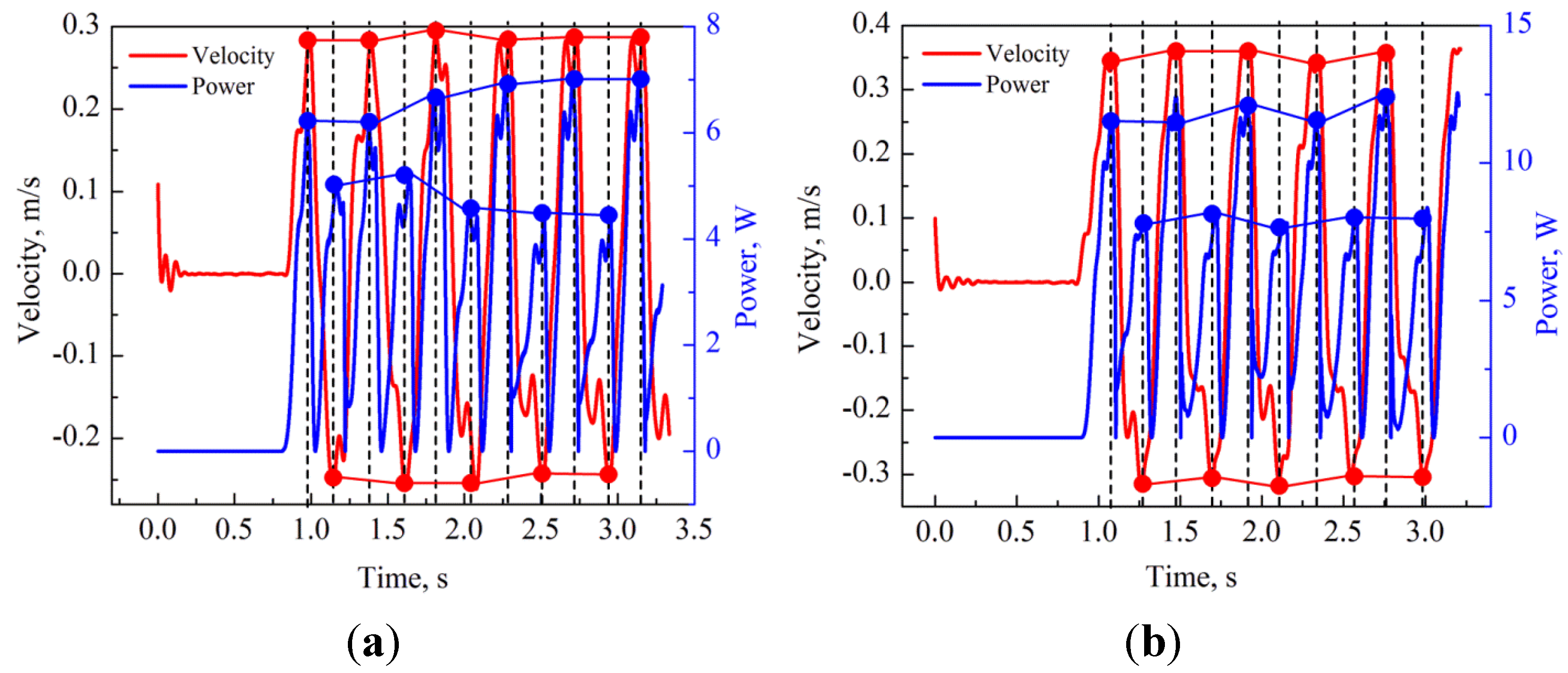
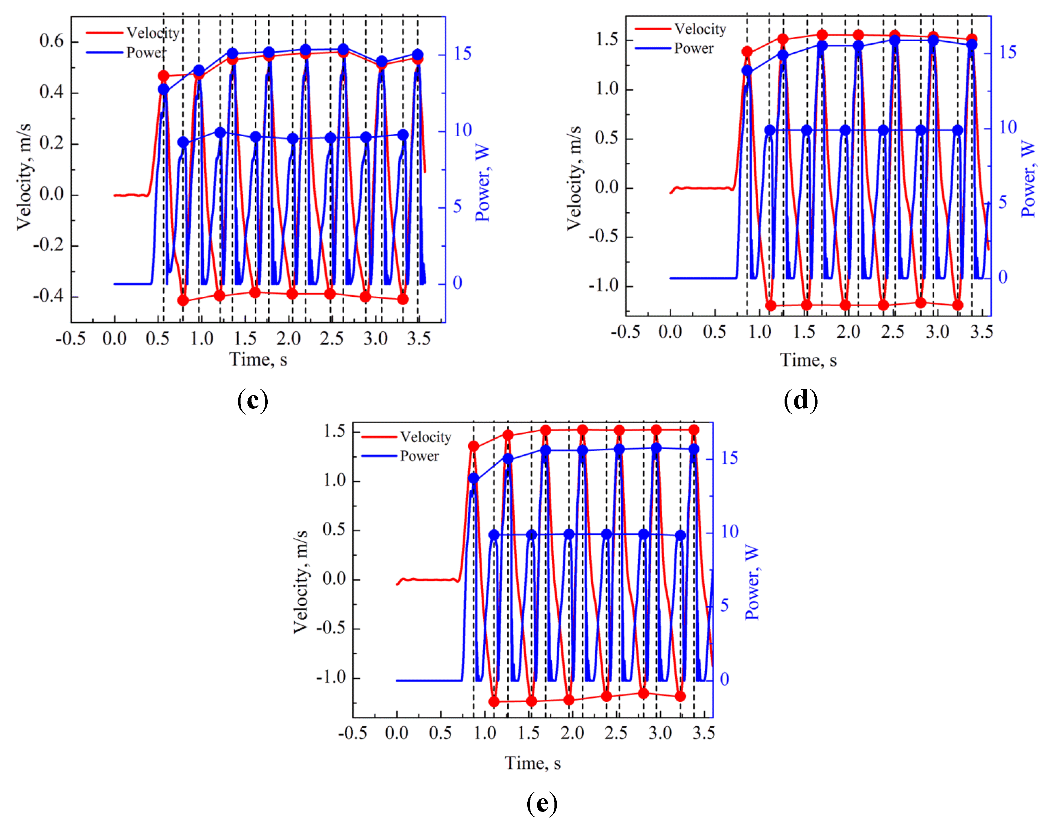
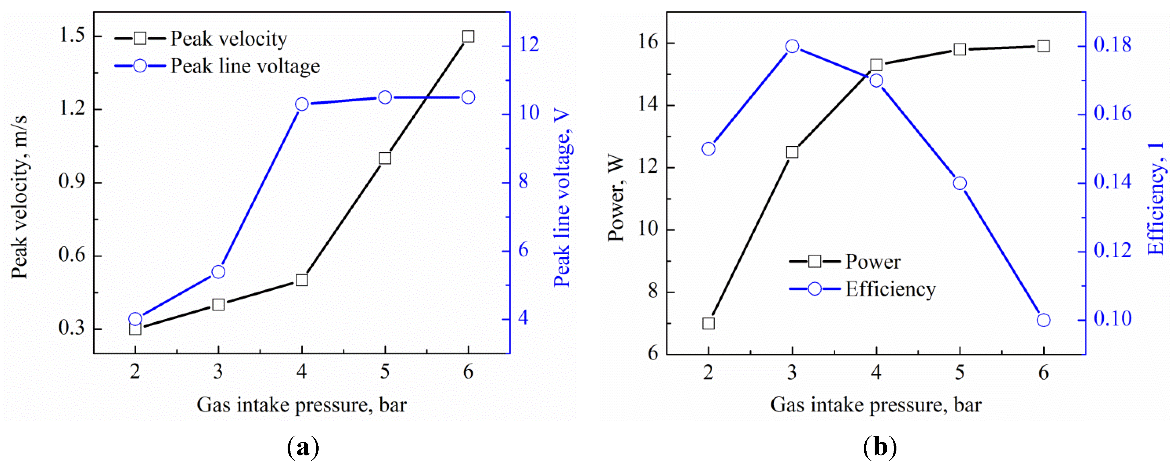
3.2.1. Variation of Intake Pressures

In this series of cases, the tests were run with a frequency of 5 Hz, a load resistance of 3.5 Ω and intake pressures of 2, 3, 4, 5 and 6 bar. The results are shown in Figure 9. Figure 9a–e are the velocities of the piston and the output power of the linear generator in which the reciprocating movement process of the free piston was continuous. The velocity reached a maximum at the midpoint of the stroke. In Figure 9a,b, the maximum velocity and peak output power were not stable after the starting process, but they stabilized when the intake pressure increased to 4 bar (Figure 9c). As the intake pressure continued to increase, the state of motion became steady, as did the generated power. Therefore, to ensure stable operation of the system, sufficiently high gas intake pressure was required.

Figure 9. (a) 2 bar intake pressure; (b) 3 bar intake pressure; (c) 4 bar intake pressure; (d) 5 bar intake pressure; (e) 6 bar intake pressure.

Figure 9. (a) 2 bar intake pressure; (b) 3 bar intake pressure; (c) 4 bar intake pressure; (d) 5 bar intake pressure; (e) 6 bar intake pressure.

At 2 bar, the maximum velocity was less than 0.3 m/s, at 3 bar, less than 0.4 m/s, at 4, 5 and 6 bar, approximately 0.5, 1.0 and 1.5 m/s, respectively.

Figure 10. (a) The peak velocity and peak line voltage at different intake pressures; (b) The generating power and efficiency at different intake pressures.

Figure 10. (a) The peak velocity and peak line voltage at different intake pressures; (b) The generating power and efficiency at different intake pressures.

With increasing intake pressure, the maximum velocity of the reciprocating piston increased; this meant that the variation trends of peak velocity and output power were basically the same. Peak velocity and peak line voltage at different intake pressures are illustrated in Figure 10. In Figure 9, the induction electromotive force of the linear generator is strongly related to the motor speed, and the energy conversion is apparent at the moment of peak velocity. However, with the increase of intake pressure, the line voltage increases. When the intake pressure changes from 4 to 5 bar, there is an obvious rise of the peak line voltage. As the intake pressure is changed from 4 to 5 and 6 bar, the value of peak line voltage converges to approximately 10 V. Although the peak piston velocity increases greatly as the gas intake pressure rises, the peak line voltage does not increase in an obvious way. As the coloured line graph shows in Figure 10b, there is a maximum value of efficiency when the gas intake pressure is 3 bar, but the power does not rise appreciably. We conclude that this phenomenon is caused by the performance of the linear generator, whose primary section is composed of numbers of coils. According to the power process illustrated in Section 3.1, the electricity generating efficiency can be calculated as follows:

$${\text{η}}_{\text{efficiency}}=\frac{E_{\text{generating}}}{W_{\text{gas}}+E_{\text{motor}}}$$

(20)

where ${\text{η}}_{\text{efficiency}}$ means electricity generating efficiency, $E_{\text{generating}}$ is the output electricity energy, $E_{\text{gas}}$ is gas acting work, and $E_{\text{motor}}$ is input electricity energy of linear motor. All the values of previous parameters are calculated in the same cycles. When the gas intake pressure is higher than 4 bar, the electrical generating efficiency diminishes because of resistance due to heat. Therefore, the power decreases sharply when the gas intake pressure is greater than 4 bar.

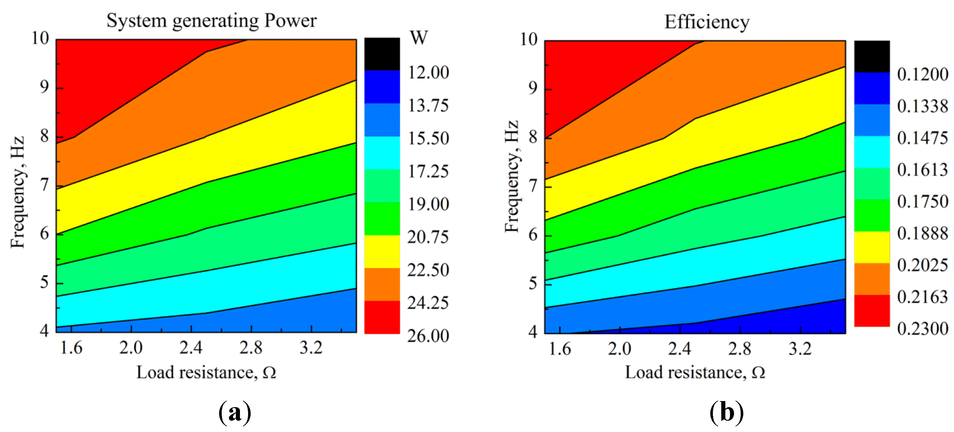
3.2.2. Variation of Frequency

Measurements were made for three conditions of performing work. The intake pressure was 5 bar in all cases; the load resistances were 1.5, 2.5 and 3.5 Ω. For each condition, the frequency was set to 10, 6.7, 5 and 4 Hz. The frequency and load resistance characteristics are shown in Figure 9.

The line voltage rises with the increase of frequency (Figure 11) because it is directly proportional to velocity. Although the intake pressure was constant, the system frequency could be changed by setting the frequency of the motor rebound force. The input energy of every cycle was equal. As Figure 11b shows, the parameters of frequency and load resistance can be adjusted to achieve the special peak of line voltage, power, and efficiency. If the objective power or peak line voltage cannot be reached by setting the frequency, the load resistance can be changed. For example, when the frequency was 5 Hz and the load resistance was 1.5 Ω, the peak line voltage was 13 V. When the frequency was changed to 10 Hz, to keep the line voltage as 13 V, the load resistance could be changed to 3.5 Ω as the dotted line shows in Figure 11a. Similarly, the power and efficiency can be kept constant to adjust the load resistance and frequency as the dotted line shows in Figure 11b. This is one of the ways to control the system to keep it stable. However, as the curves in Figure 11 show, even if the input energy is equal in these cases at the same intake pressure, there is an extreme value of peak line voltage as the load resistance increases.

Figure 11. (a) The peak line voltage at different frequencies; (b) The generated power and efficiency at different frequencies.

Figure 11. (a) The peak line voltage at different frequencies; (b) The generated power and efficiency at different frequencies.

Firstly, the frequency has a strong relationship with load resistance, although the frequency can be regulated by changing the controlling program for gas intake pressure and the linear motor rebound force. As a supplement, Figure 12 shows contour maps of power and efficiency at various values of frequency and load resistance. The trends of variations of system generating power and efficiency look roughly the same. We note that the power and efficiency of the system can achieve high values together by adjusting the load resistance and frequency. The load resistance characteristics will be discussed in the section below.

Figure 12. (a) System generating power, and (b) efficiency at various load resistances and frequencies.

Figure 12. (a) System generating power, and (b) efficiency at various load resistances and frequencies.

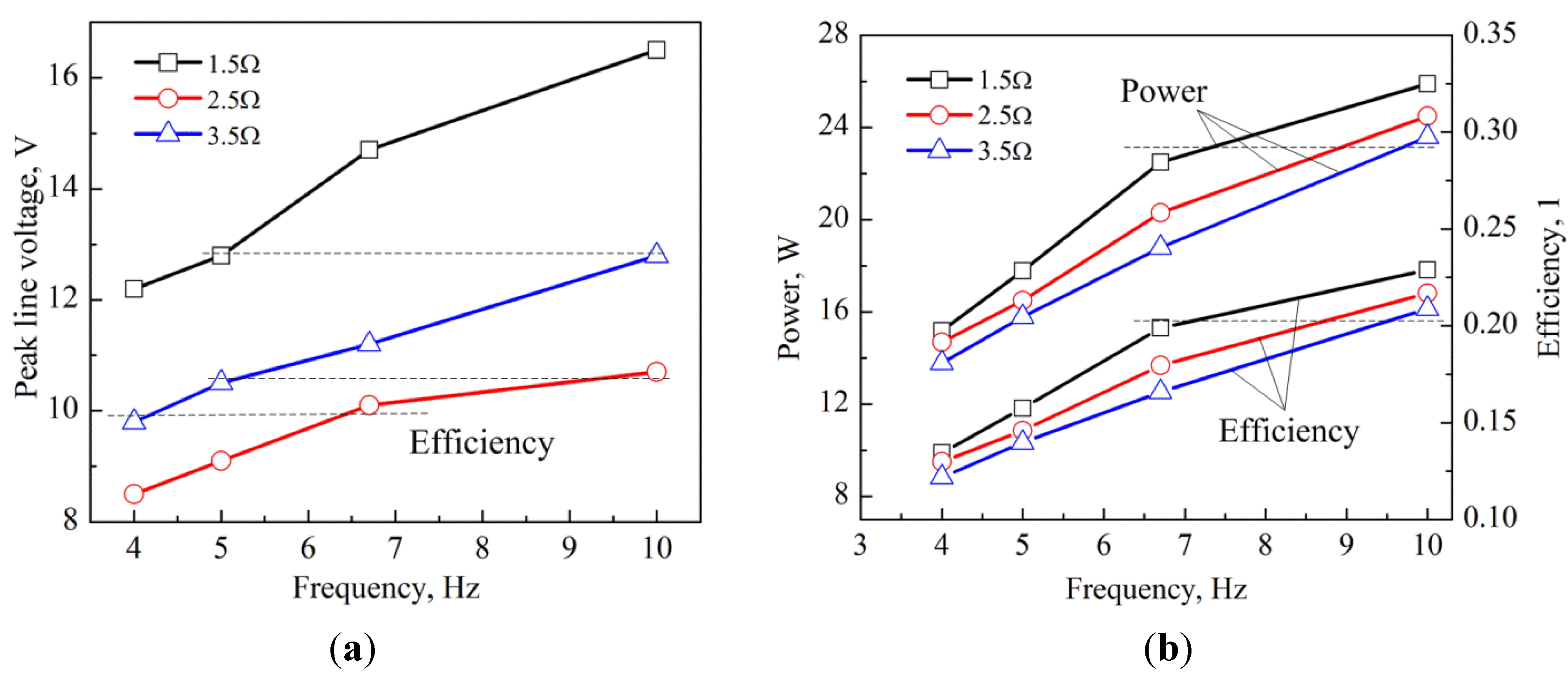
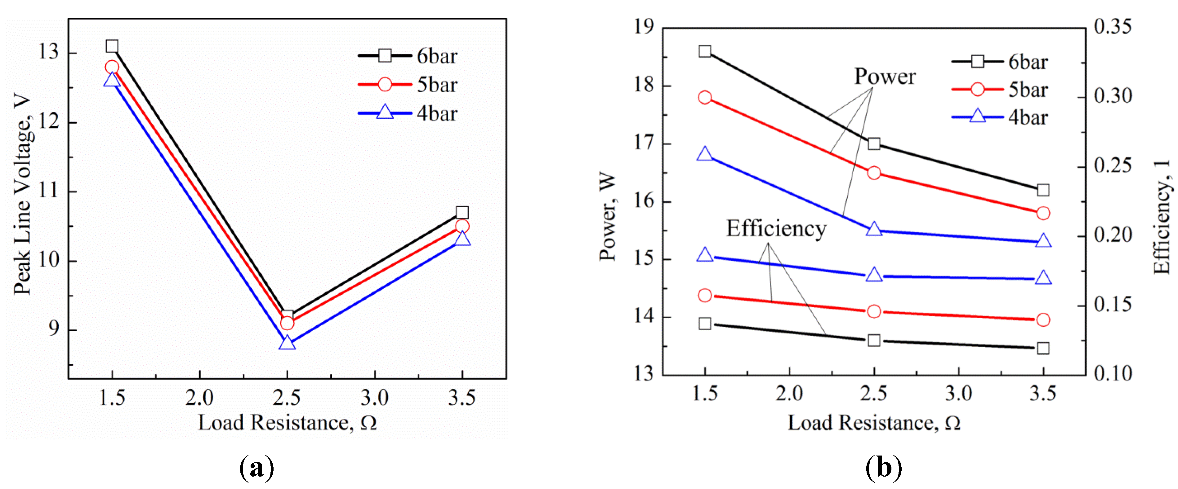
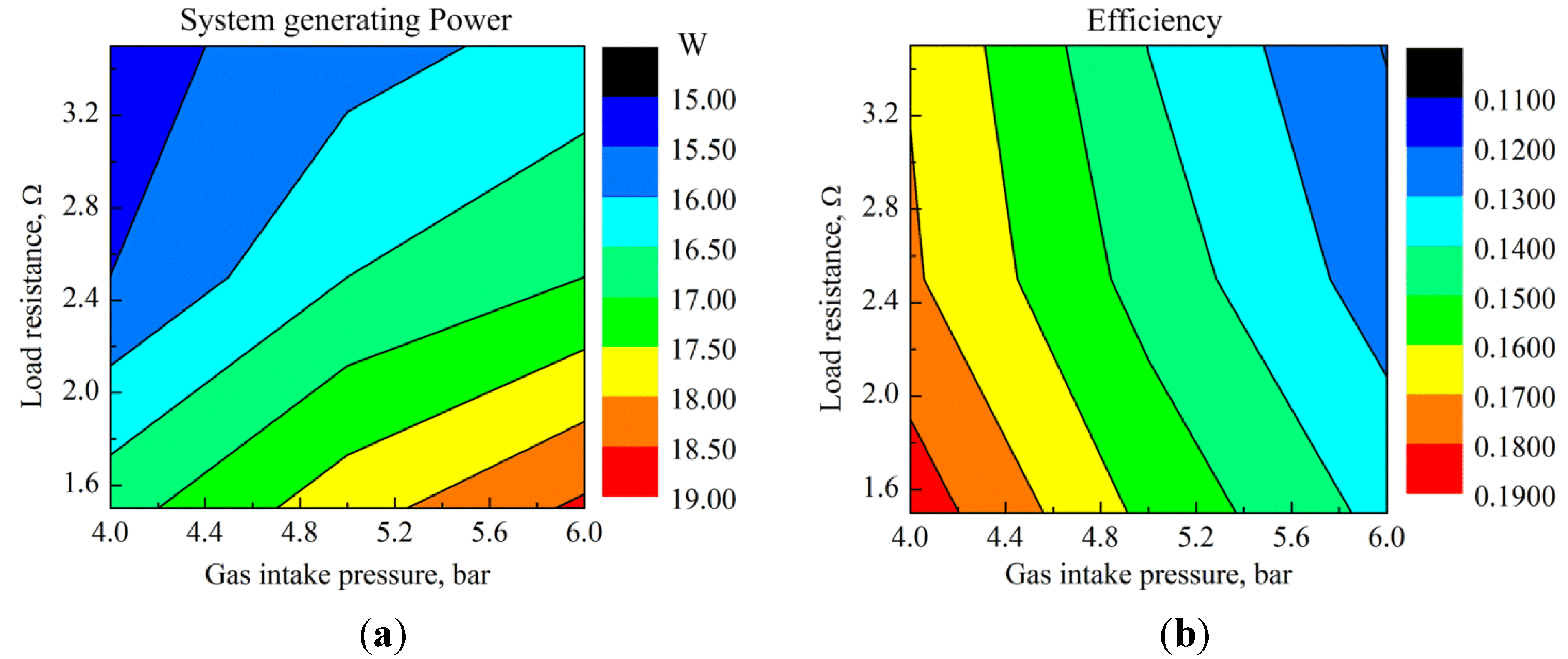
3.2.3. Variation of Load Resistance

Load resistance is a special parameter that not only measures the system output energy, but also influences the system dynamical performance. It is directly related to Fe (electromagnetic force in Equation (1)) produced by the linear generator. In this series of tests, the frequency was set to 5 Hz, and the load resistances were set at 1.5, 2.5 and 3.5 Ω. The peak line voltages, power, and efficiency with different load resistances are shown in Figure 13.

Figure 13. (a) The peak line voltage with different load resistance; (b) The power and efficiency in different load resistance.

Figure 13. (a) The peak line voltage with different load resistance; (b) The power and efficiency in different load resistance.

As noted above, the load characteristic of the system is special. The load resistance is not directly related to the peak line voltage. At a load resistance of 2.5 Ω (Figure 13a), the peak line voltage is a minimum. However, the system generating power and efficiency always decline with increasing load resistance (Figure 13b). The trends of generated power and efficiency with change of load resistance are similar. However, with increasing gas intake pressure, the trend of generated power is completely different from that of efficiency. This can be verified in Figure 14. With high gas intake pressure and low load resistance, generated power can reach 18.6 W. With low gas intake pressure and load resistance, the efficiency can reach 18.58%. With these conclusions, that higher power and efficiency cannot be controlled with the gas intake pressure, the load resistance can be set to the appropriate value to balance system generated power and efficiency. If we wish to change the load resistance to control the peak line voltage within a limited range, there is a minimal value of peak line voltage. Because the linear generator always has the lowest safety voltage, we should adjust the load resistance to make the peak line voltage lower than the safety voltage.

Figure 14. (a) The system generating power contour with varied load resistance and gas intake pressure; (b) The efficiency with varied load resistance and gas intake pressure.

Figure 14. (a) The system generating power contour with varied load resistance and gas intake pressure; (b) The efficiency with varied load resistance and gas intake pressure.

4. Conclusions

In this paper, a detailed simulation model that simulates the stable operating process of a single-cylinder FPELG with various patterns of linear motor rebound force is described. The simulation conclusions were used in experiments which were performed to investigate the generating characteristics of a linear generator. The behaviour found experimentally can be applied in researching the adaptability of the device in various operating modes.

(1)

In the simulation, the peak value of displacement increases with the increase of motor rebound force. There is a minimal value of brake output power when the motor rebound force is approximately 500 N. When the motor rebound position increases, the maximum displacement and brake output power of the linear generator both increase.

(2)

Compared to a motor rebound force with a triangular profile, a parabolic motor rebound force profile has advantages such as higher values of the maximum positive velocity, shorter time to reach the TDC, and higher peak cylinder pressure.

(3)

Experimentally, the maximum velocities and peak output power were not stable after the starting process until the intake pressure reached 4 bar. As the gas intake pressure increased, the system output power rose continually. However, the system reached its maximum efficiency before reaching maximum output power, which rose slowly.

(4)

The parameters of frequency and load resistance could be adjusted to achieve a special peak line voltage, peak power, and efficiency, which is one of the ways to control the system. The output power reached 25.9 W and the system efficiency reached 13.7%.

References

1. Mikalsen, R.; Roskilly, A.P. Performance simulation of a spark ignited free-piston engine generator. Appl. Ther. Eng. 2008, 28, 1726–1733. [Google Scholar] [CrossRef]
2. Mao, J.; Zuo, Z.; Feng, H. Parameters coupling designation of diesel free-piston linear alternator. Appl. Energy 2011, 88, 4577–4589. [Google Scholar] [CrossRef]
3. Mikalsen, R.; Roskilly, A.P. A review of free-piston engine history and applications. Appl. Therm. Eng. 2007, 27, 2339–2352. [Google Scholar] [CrossRef]
4. Mikalsen, R.; Jones, E.; Roskilly, A.P. Predictive piston motion control in a free-piston internal combustion engine. Appl. Energy 2010, 87, 1722–1728. [Google Scholar] [CrossRef]
5. Mao, J.; Zuo, Z.; Liu, D. Numerical Simulation of a Spark Ignited Two-Stroke Free-Piston Engine Generator. J. Beijing Inst. Technol. 2009, 18, 283–287. [Google Scholar]
6. Mikalsen, R.; Roskilly, A.P. The control of a free-piston engine generator. Part 1: Fundamental analyses. Appl. Energy 2010, 87, 1273–1280. [Google Scholar] [CrossRef]
7. Li, Q.; Jin, X.; Huang, Z. Simulation of a two-stroke free-piston engine for electrical power generation. Energy Fuels 2008, 22, 3443–3449. [Google Scholar] [CrossRef]
8. Pescara, R.P. Motor Compressor Apparatus. U.S. Patent 1,657,641, 31 January 1928. [Google Scholar]
9. Atkinson, C.M.; Petreanu, S.; Clark, N.N. Numerical simulation of a two-stroke linear engine. SAE Paper 1999. [Google Scholar] [CrossRef]
10. Goldsborough, S.S.; Blarigan, P.V. A numerical study of a free-piston IC engine operation on homogeneous charge compression ignition combustion. SAE Paper 1999. [Google Scholar] [CrossRef]
11. Nemecek, P.; Vysoky, O. Control of two-stroke free-piston generator. In Proceeding of the 6th Asian Control Conference, Bali, Indonesia, 18–21 July 2006.
12. Mikalsen, R.; Roskilly, A.P. The design and simulation of a two-stroke free-piston compression ignition engine for electrical power generation. Appl. Therm. Eng. 2008, 28, 589–600. [Google Scholar] [CrossRef]
13. Mikalsen, R.; Roskilly, A.P. The control of a free-piston engine generator. Part 2: Engine dynamics and piston motion control. Appl. Energy 2010, 87, 1281–1287. [Google Scholar] [CrossRef]
14. Kosaka, H.; Akita, T.; Moriya, K. Development of free piston engine linear generator system Part 1—Investigation of fundamental characteristics. SAE Tech. Paper 2014. [Google Scholar] [CrossRef]
15. Goto, S.; Moriya, K.; Kosaka, H. Development of free piston engine linear generator system Part 2—Investigation of control system for generator. SAE Tech. Paper 2014. [Google Scholar] [CrossRef]
16. Kim, J.; Bae, C.; Kim, G. Simulation on the effect of the combustion parameters on the piston dynamics and engine performance using the Wiebe function in a free piston engine. Appl. Energy 2013, 107, 446–455. [Google Scholar] [CrossRef]
17. Zhao, Z.; Zhang, F.; Huang, Y. An experimental study of the cycle stability of hydraulic free-piston engines. Appl. Ther. Eng. 2013, 54, 365–371. [Google Scholar] [CrossRef]
18. Mao, J.; Zuo, Z.; Li, W. Multi-dimensional scavenging analysis of a free-piston linear alternator based on numerical simulation. Appl. Energy 2011, 88, 1140–1152. [Google Scholar] [CrossRef]
19. Hohenberg, G.F. Advanced approaches for heat transfer calculations. SAE Paper 1979. [Google Scholar] [CrossRef]
20. Rosengerg, R. General friction considerations for engine design. SAE Paper 1982. [Google Scholar] [CrossRef]
21. Chiang, C.; Yang, J.; Lan, S. Dynamic modeling of a SI/HCCI free-piston engine generator with electric mechanical valves. Appl. Energy 2013, 102, 336–346. [Google Scholar] [CrossRef]
22. Zhu, Y.; Wang, Y.; Zhen, X. The control of an opposed hydraulic free piston engine. Appl. Energy 2014, 126, 213–220. [Google Scholar] [CrossRef]
23. Tang, Y.; Shi, N. Electric Machinery, 2nd ed.; China Machine Press: Beijing, China, 2005. [Google Scholar]
24. Hung, N.B.; Lim, O.T. A study of a two-stroke free piston linear engine using numerical analysis. J. Mech. Sci. Technol. 2014, 28, 1545–1557. [Google Scholar] [CrossRef]