Pareto-Optimal Evaluation of Ultimate Limit States in Offshore Wind Turbine Structural Analysis

Abstract

The ultimate capacity of support structures is checked with extreme loads. This is straightforward when the limit state equations depend on a single load component, and it has become common to report maxima for each load component. However, if more than one load component is influential, e.g., both axial force and bending moments, it is not straightforward how to define an extreme load. The combination of univariate maxima can be too conservative, and many different combinations of load components can result in the worst value of the limit state equations. The use of contemporaneous load vectors is typically non-conservative. Therefore, in practice, limit state checks are done for each possible load vector, from each time step of a simulation. This is not feasible when performing reliability assessments and structural optimization, where additional, time-consuming computations are involved for each load vector. We therefore propose to use Pareto-optimal loads, which are a small set of loads that together represent all possible worst case scenarios. Simulations with two reference wind turbines show that this approach can be very useful for jacket structures, whereas the design of monopiles is often governed by the bending moment only. Even in this case, the approach might be useful when approaching the structural limits during optimization.

1. Introduction

The design of offshore wind turbines and their support structures is based on load simulations, in which the response of the turbine to the different loads encountered in its environment is simulated and assessed [1]. Loads typically consist of wind and wave loads, and the relevant standards prescribe a large number of load cases and scenarios that have to be evaluated [2]. The validity of the design is then checked regarding fatigue damage, ultimate capacity and compliance with other criteria, such as service limits and behavior under accident conditions (e.g., ship collisions).

In this short note, we consider only the ultimate limit state (ULS) and, more specifically, its assessment for the support structure of a fixed-bottom wind turbine, such as a monopile or a jacket foundation. The standard assessment is based on a hybrid approach, in which both operational load cases, e.g., International Electrotechnical Commission (IEC) Design Load Case (DLC) 1.1: power production under normal turbulence, as well as extreme load cases, e.g., IEC DLC 1.3: power production under extreme turbulence and DLC 6.1: idling under extreme wind speed and/or extreme sea state, are considered. It is traditional in engineering to report the extreme loads acting on the wind turbine in an ultimate loads table, first for each load case and then as a summary over all load cases. These tables, one for each load case, show both the minimum and maximum values for each degree of freedom (forces $F_x$, $F_y$, $F_z$ and moments $M_x$, $M_y$, $M_z$) acting on a specific location of the wind turbine, typically the tower bottom. The summary table identifies for each of these degrees of freedom the load case with the highest load in this particular variable and reports the minima and maxima of all of the other variables in the same load case (Table 4-2 in [3] is a typical example). Apart from total loads on the structure, also the stress resultants for each structural detail or member can be reported in such a format. For a tubular member modeled as a beam, these consist of axial force $F_x$ and the two bending moments $M_y$ and $M_z$ (Table 1). These tables are used extensively in the preliminary design of support structures. During the final design phase, the loads on the support structure are then assessed for each simulated time step individually, and extensive code checks are performed in which the ULS condition is evaluated.

Table 1. Example ultimate loads table. This shows typical results from a structural response analysis for a brace member at the bottom of the Offshore Code Comparison Collaboration Continuation (OC4) jacket support structure. Both contemporaneous loads (for each variable) and the standard approach using univariate maxima/minima are shown, the latter in the two bottom rows. These numbers correspond with the time series shown in Figure 1. F, force; M, moment.

Variable		$F_x$	$M_y$	$M_z$	$M_{yz}$
		(MN)	(MNm)	(MNm)	(MNm)
$F_x$	Maximum	8.542	−0.298	−0.069	0.306
	Minimum	5.317	−0.013	0.248	0.248
$M_x$	Maximum	6.537	0.140	0.389	0.414
	Minimum	7.204	−0.434	−0.229	0.490
$M_y$	Maximum	6.537	0.140	0.389	0.414
	Minimum	7.204	−0.434	−0.229	0.490
$M_{xy}$	Maximum	7.204	−0.434	−0.229	0.490
	Minimum	5.670	−0.087	−0.089	0.125
Overall	Maximum	8.542	0.140	0.389	0.490
	Minimum	5.317	−0.434	−0.229	0.125

Table 1. Example ultimate loads table. This shows typical results from a structural response analysis for a brace member at the bottom of the Offshore Code Comparison Collaboration Continuation (OC4) jacket support structure. Both contemporaneous loads (for each variable) and the standard approach using univariate maxima/minima are shown, the latter in the two bottom rows. These numbers correspond with the time series shown in Figure 1. F, force; M, moment.

Variable		$F_x$	$M_y$	$M_z$	$M_{yz}$
		(MN)	(MNm)	(MNm)	(MNm)
$F_x$	Maximum	8.542	−0.298	−0.069	0.306
	Minimum	5.317	−0.013	0.248	0.248
$M_x$	Maximum	6.537	0.140	0.389	0.414
	Minimum	7.204	−0.434	−0.229	0.490
$M_y$	Maximum	6.537	0.140	0.389	0.414
	Minimum	7.204	−0.434	−0.229	0.490
$M_{xy}$	Maximum	7.204	−0.434	−0.229	0.490
	Minimum	5.670	−0.087	−0.089	0.125
Overall	Maximum	8.542	0.140	0.389	0.490
	Minimum	5.317	−0.434	−0.229	0.125

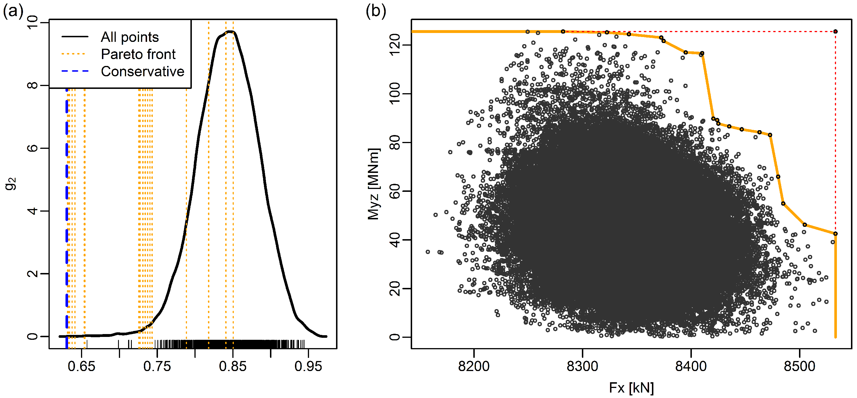
This approach has two important limitations, both of which are addressed here. First, the ultimate loads table gives the impression that the maxima of individual loads appear together at the same time, which is normally not the case. Figure 1 illustrates this for axial forces and bending moments in a joint of a jacket structure (at the location indicated in Figure 2). The maximum of the axial force is obtained at time $t_1=183.75$ s (Figure 1a), whereas the maximum of the total bending moment is obtained at time $t_2=63.275$ s (Figure 1b). In both cases, the other variable takes on significantly lower values than one can infer from the ultimate loads table. This means that reporting all individual maxima together leads to a conservative assessment of the loads. This limitation has been addressed in the last revision of the IEC 61400-1 standard [4], where Appendix H advocates the use of contemporaneous loads: for each variable, the maximum/minimum is determined and combined with the values of the other variables at the same time (see Table 1 for an example). However, as will be shown below, this approach is typically non-conservative.

The other limitation is that, when the actual loads are used, the amount of data that needs to be processed tends to be very large. This is of particular concern when one tries to assess the structural reliability of the support structure [5]. In this case, one has to perform a probabilistic assessment, in which the various uncertainties about the design, the loads and the materials have to be considered. A straightforward way is a Monte Carlo simulation in which variations of important parameters, e.g., the steel yield strength, are randomly generated. These parameters are then used together with the loads in a limit state equation, and the probability of structural failure is evaluated by determining how many of these samples result in values that are outside of the safe region. As this is a time-consuming process, it cannot be performed for each time step individually.

There is thus a need for a more representative overview of the defining loads in wind turbine structural analysis. This is addressed here by introducing the concept of Pareto-optimal loads. These are defined in Section 2, which also discusses typical ULS functions and presents details about the computational model used for a demonstration. Section 3 presents some exemplary results from a simplified analysis of both a monopile and a jacket support structure. Finally, the findings are summarized and discussed in Section 4.

Figure 1. Illustration of the difference between Pareto-optimal loads and the standard approach for the bottom joint in the OC4 jacket support structure, at rated wind speed. (a) axial force. (b) total bending moment. The broken red lines indicate the locations and values of the univariate maxima. (c) limit state function for combined bending and compression (Equation (5)). The broken red line indicates the value for the conservative combination of univariate maxima. The dotted orange lines indicate the locations and values at the Pareto-optimal points. Note that only a small part of the total time series has been shown, for the purposes of better visualization.

Figure 1. Illustration of the difference between Pareto-optimal loads and the standard approach for the bottom joint in the OC4 jacket support structure, at rated wind speed. (a) axial force. (b) total bending moment. The broken red lines indicate the locations and values of the univariate maxima. (c) limit state function for combined bending and compression (Equation (5)). The broken red line indicates the value for the conservative combination of univariate maxima. The dotted orange lines indicate the locations and values at the Pareto-optimal points. Note that only a small part of the total time series has been shown, for the purposes of better visualization.

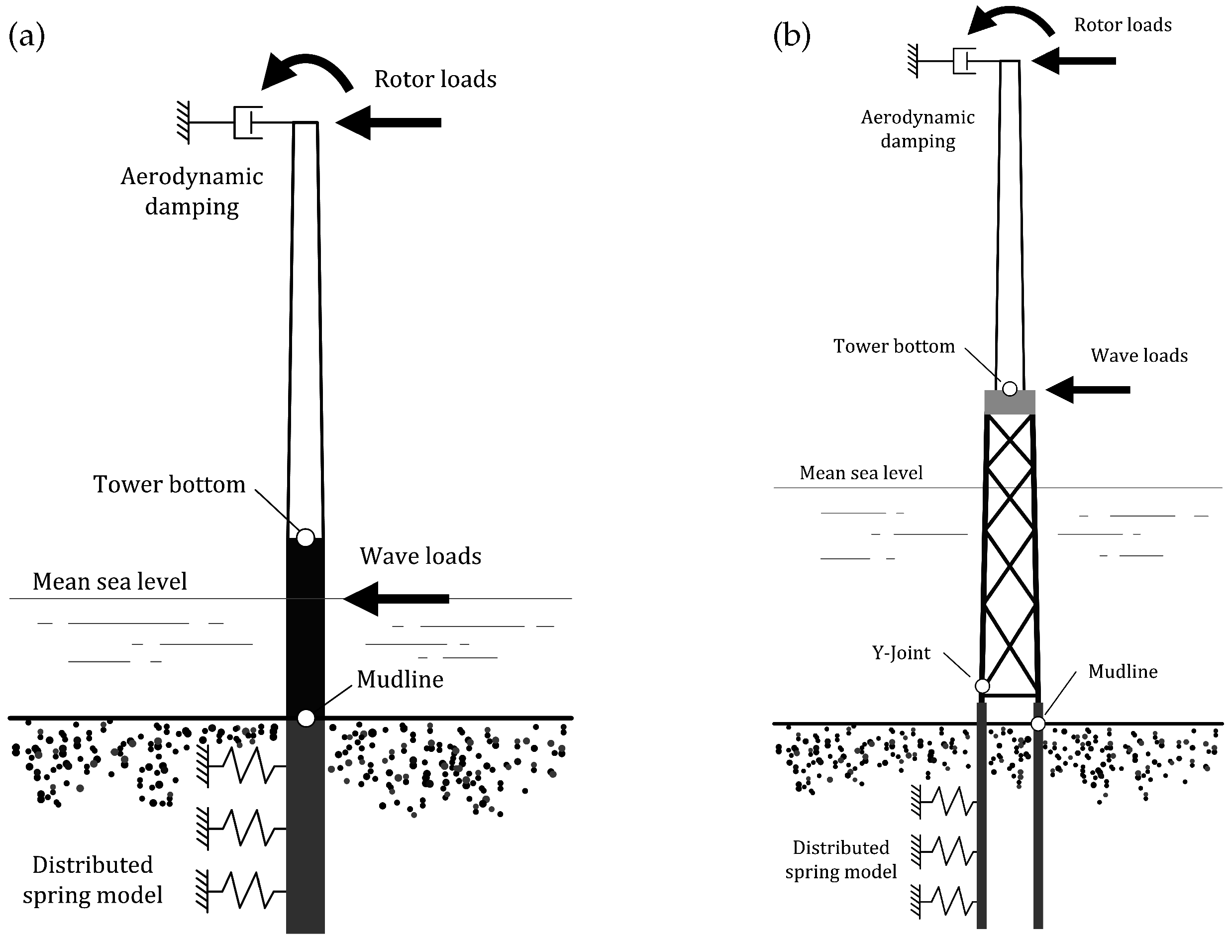
Figure 2. Illustration of numerical models used for example calculations. (a) OC3 monopile. (b) OC4 jacket with additional soil model. Output locations are indicated.

Figure 2. Illustration of numerical models used for example calculations. (a) OC3 monopile. (b) OC4 jacket with additional soil model. Output locations are indicated.

2. Methods

2.1. Pareto-Optimal Loads

The concept of Pareto optimality is a generalization of the idea of the maximum value. The basis of both concepts is an ordering of elements. When confronted with a univariate (one-dimensional) record of n observations $x^{\left(1\right)},x^{\left(2\right)},\cdots ,x^{\left(n\right)}$, the standard order relation for numerical values (denoted by $x\le y$) allows one to sort the samples according to their size and thereby identifies a maximal element $x^{\left(\max \right)}$, which has the defining property that:

$$x^{\left(i\right)}\le x^{\left(\max \right)}\text{for}\text{all}i=1,2,\cdots ,n$$

When confronted with a multivariate record, i.e., a number of d-dimensional vectors $x^{(i)}=(x_1^{(i)},x_2^{(i)},\cdots ,x_d^{(i)})$ of observations, it is not immediately clear how to order these. In fact, typically, no linear order exists, i.e., there exists no simple order relationship that allows one to compare each element with each other in a consistent way. The straightforward generalization of the order $x\le y$ for univariate records to d-dimensional observations is to define:

$$x=(x_1,x_2,\cdots ,x_d)\le (y_1,\cdots ,y_d)=y\text{if}{x}_i\le y_i\text{for}\text{all}i=1,2,\cdots ,d$$

In other words, a vector x is less or equal to a vector y if all elements of x are less or equal to all corresponding elements in the vector y. We say that the vector y dominates the vector x.

This dominance order, unfortunately, only defines a partial order, i.e., there exist many combinations of elements that cannot be compared. The concept of a maximal element still exists, if we define a maximal element as an $x^{*}$, such that:

$$\text{if}{x}^{*}\le y\text{for}\text{some}\text{element}y,\text{then}y=x^{*}$$

or in other words, there exists no other observation that dominates x. However, now, the maximum is not unique anymore, and there can be many maximal elements.

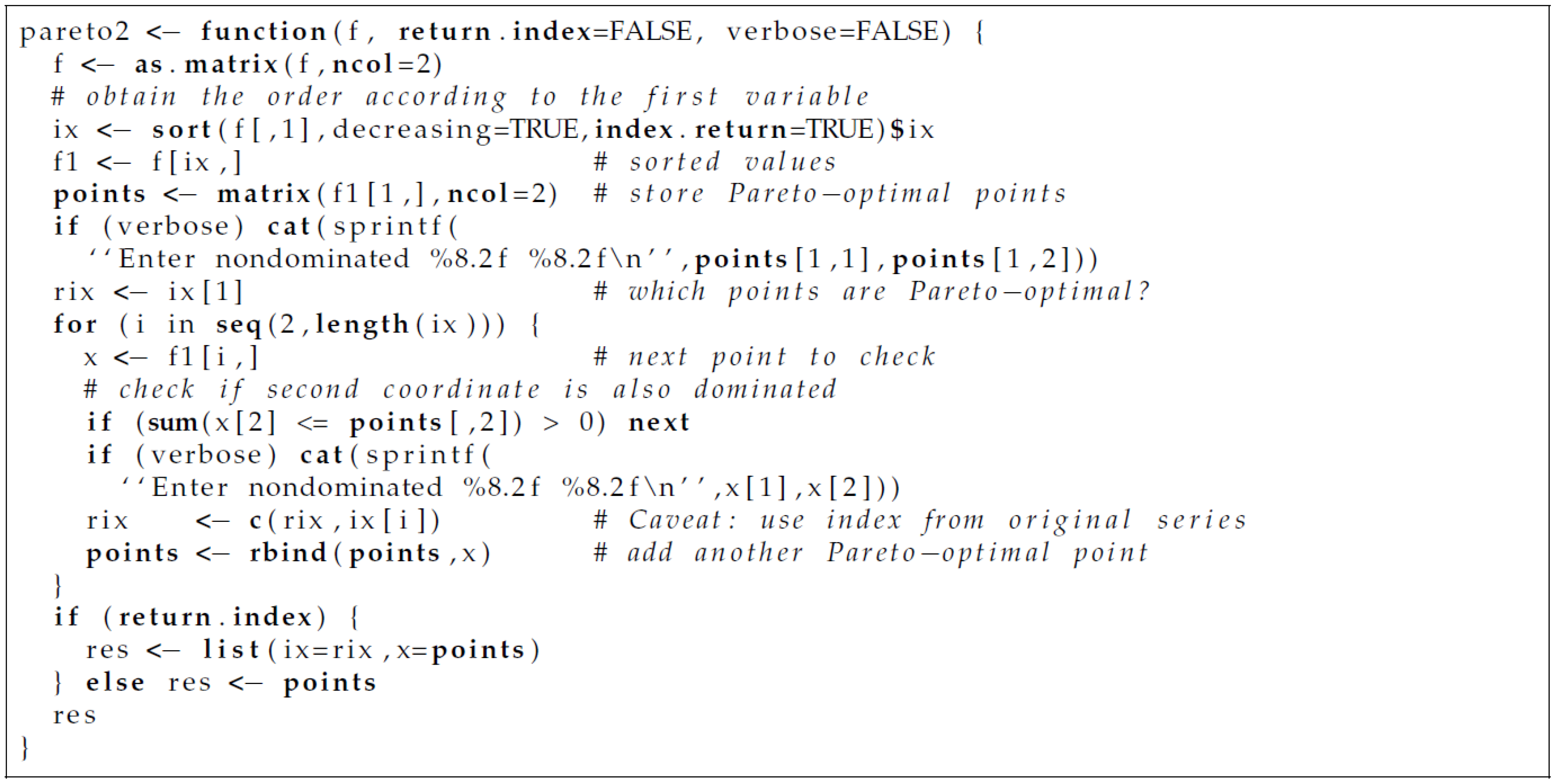
Finding all Pareto-optimal elements is easily done by iterating through all observations. The most important cases in practice are for two- and three-dimensional vectors of observations (e.g., axial force and the two bending moments in a structural member). The straightforward algorithms are given in the Appendix, for use with the open-source statistical analysis software R [6], and can be easily adapted into other programming or scripting languages.

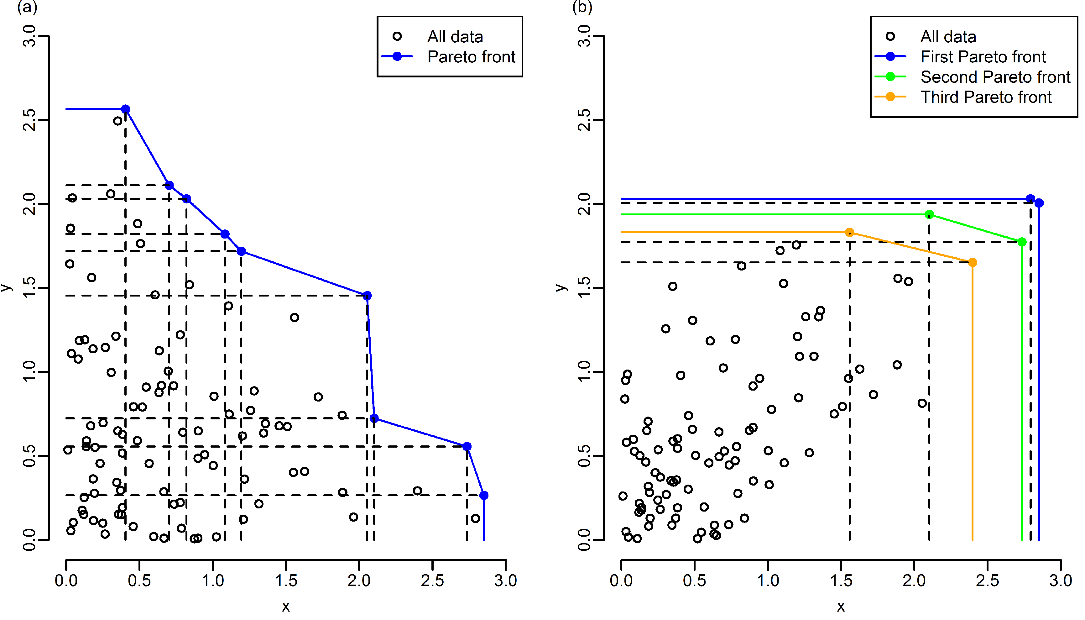
Let us illustrate the method with an example. Figure 3a shows a scatterplot of $(x,y)$ pairs, where the two elements in each observation have been generated randomly and independently, from a standard Gaussian distribution (for simplicity, only elements with positive values are shown). The elements in blue are the maximal elements. For each of them, the broken lines indicate the regions that are dominated by them. Together, the blue elements form the so-called Pareto front. As can be seen, a relatively small number of such Pareto-optimal elements (nine points, to be precise) covers the entire dataset (consisting of 100 points).

Figure 3b shows a similar scatterplot of $(x,y)$ pairs, where now, a significant positive correlation exists between the x- and y-values. In this case, the Pareto front is rather simple and consists of only two elements. As the figure illustrates, it is also possible to define higher-order Pareto fronts. These are determined by successively removing all elements from the Pareto front and then finding the Pareto-optimal elements of the remaining points. Repeating this process, the first three Pareto fronts so obtained are shown in the figure.

The concept of Pareto optimality is used extensively in economic analysis and multi-criteria optimization, including structural optimization (see, e.g., [7,8,9]).

Figure 3. Illustration of Pareto optimality. (a) Samples from two independent Gaussian distributions. The Pareto front consists of the blue points. The broken lines show the regions of the space that are dominated by each Pareto-optimal point. (b) Samples from two strongly-correlated Gaussian distributions. A number of higher-order Pareto fronts are indicated as well (see the text for details).

Figure 3. Illustration of Pareto optimality. (a) Samples from two independent Gaussian distributions. The Pareto front consists of the blue points. The broken lines show the regions of the space that are dominated by each Pareto-optimal point. (b) Samples from two strongly-correlated Gaussian distributions. A number of higher-order Pareto fronts are indicated as well (see the text for details).

2.2. Ultimate Limit State Equations

Whether a design fulfills the ULS condition is assessed by performing a number of checks. The structure of these tests is highly standardized. Typically, a limit-state equation is used, and values of the limit-state equation below zero signify structural failure.

The relevant standards specify a vast number of such checks, and their formulations differ significantly. We consider here only the most important and common features. The following is based on the Norsk Sokkels Konkurranseposisjon (NORSOK) offshore standard “Design of Steel Structures” [10].

Focusing on tubular members, a number of checks only use univariate data. For example, each member has to be assessed for sufficient capacity to resist tensile and compressive loads and bending moments,

$$\begin{array}{cc}\hfill g_t& =\frac{A{f}_y}{{\gamma }_m}-F_x\ge 0\hfill \end{array}$$

(1)

$$\begin{array}{cc}\hfill g_c& =\frac{A{f}_c}{{\gamma }_m}-F_x\ge 0\hfill \end{array}$$

(2)

$$\begin{array}{cc}\hfill g_b& =\frac{f_{m}W}{{\gamma }_m}-M_{yz}\ge 0\hfill \end{array}$$

(3)

here, A denotes the cross-sectional area, W the elastic section modulus; γ is a material factor (with a typical value of 1.15); $f_y$ is the steel yield strength; $f_c$ is the characteristic axial compressive strength (which depends on a number of factors, such as Young’s modulus of the material and the length of the member); and $f_m$ is the characteristic bending strength (which is proportional to the yield strength). The actual loads are $F_x$ (normal force) and $M_{yz}$ (total bending moment). These univariate conditions are monotonous (in fact, linear) in the load effects $F_x$ and $M_{yz}$, and for these equations, the knowledge of the univariate maximum for each component of the loads is sufficient.

In contrast to this, a number of combined conditions exist that are often defining for the elements. We only consider compression here, being the most important condition in many cases. In the NORSOK standard, this is assessed with two limit state equations:

$$\begin{array}{cc}\hfill g_1& =1.0-\frac{F_x}{N_{c,Rd}}-\frac{1}{M_{Rd}}{\left[{\left(\frac{C_{my}{M}_y}{1-\frac{F_x}{N_{Ey}}}\right)}^2+{\left(\frac{C_{mz}{M}_z}{1-\frac{F_x}{N_{Ez}}}\right)}^2\right]}^{0.5}\ge 0\hfill \end{array}$$

(4)

$$\begin{array}{cc}\hfill g_2& =1.0-\frac{F_x}{N_{cl,Rd}}-\frac{M_{yz}}{M_{Rd}}\ge 0\hfill \end{array}$$

(5)

here, $M_{Rd}=\frac{f_{m}W}{{\gamma }_m}$ is the resistance to bending (as in Equation (3)); $N_{c,Rd}=\frac{A{f}_y}{{\gamma }_m}$ is the axial resistance to compression (as in Equation (2)), whereas $N_{cl,Rd}=\frac{A{f}_{cl}}{{\gamma }_m}$ is the resistance to local buckling. Here, the local characteristic buckling strength $f_{cl}$ depends on both the yield strength (in a non-linear way), Young’s modulus, as well as on the thickness to diameter ratio of each element. The Euler buckling strengths $N_{Ey},N_{Ez}$ depend mainly on Young’s modulus and member length, and the reduction factors $C_{my},C_{mz}$ depend on the type of structural element and details about the loading, but can be taken to be 0.85 in most cases.

Although the value of the limit state equations Equations (4)–(5) depends in a complex and nonlinear way on the load components, this relationship is monotonic for each component. In other words, larger values of either axial force or bending moment will lead to lower values of the limit state equation, all other things being kept equal. Therefore, it is clear that Pareto-optimal load vectors result in the lowest possible values of the equations, compared to the elements that are dominated by these vectors, although it is not clear which Pareto-optimal vector (i.e., which specific combination of loads) leads to the lowest value overall. In comparison, the use of contemporaneous load vectors [4] (Appendix H) is identical to the use of only two of the Pareto-optimal load vectors, the ones with the highest value for either the axial force or the bending moment.

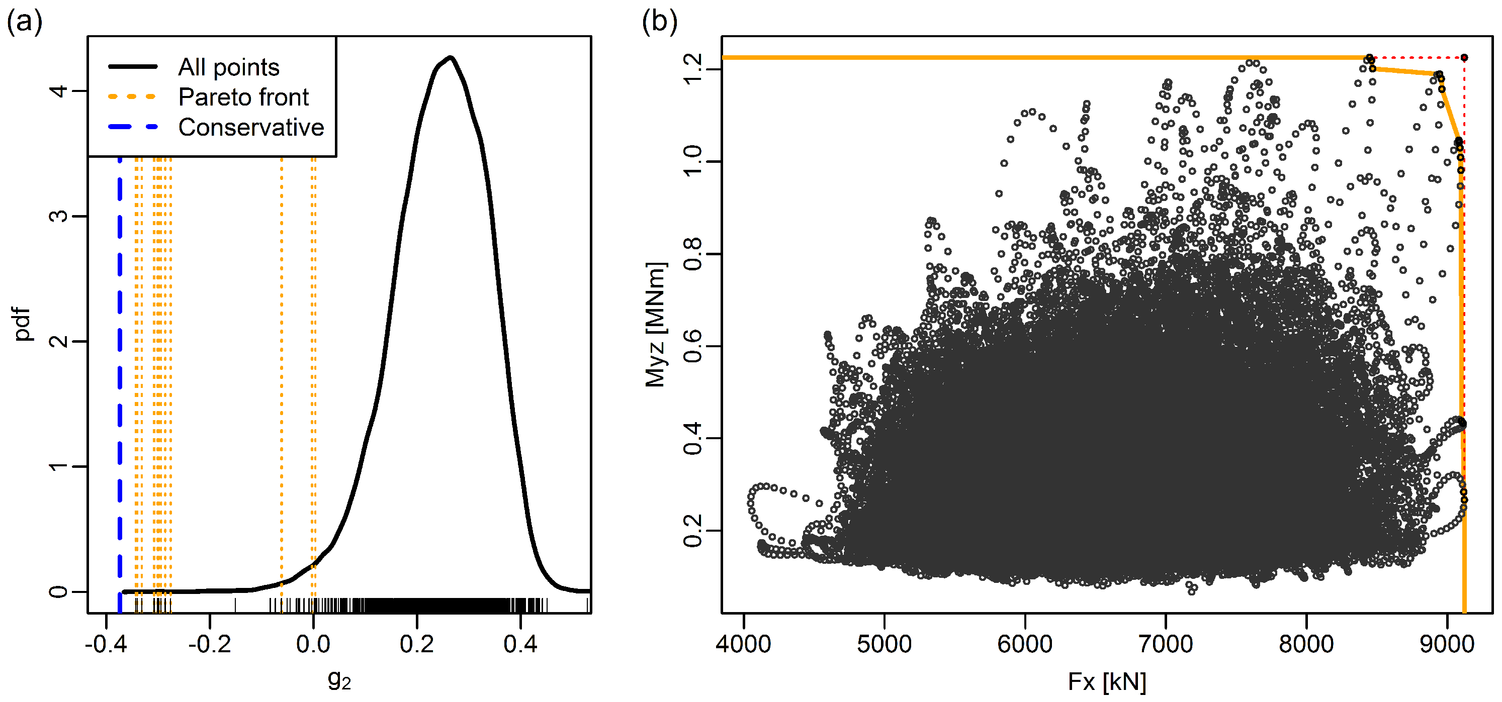
As the local characteristic buckling strength is less than the axial resistance to compression, the value of the limit state equation $g_2$ is typically lower than the corresponding value of $g_1$. For simplicity, we therefore only consider the function $g_2$ in the following examples, although a realistic application has to implement both checks. Furthermore, no (additional safety factors have been considered.

2.3. Computational Model

In order to discuss the relevance of the methodology, an example case was implemented. Two different support structures were evaluated, a monopile and a jacket support structure (Figure 2). The monopile is identical to the Offshore Code Comparison Collaboration (OC3) monopile developed within the International Energy Agency (IEA) Task 23 [11]. The jacket structure is the OC4 jacket developed within IEA Task 30 [12], but for more realistic results, a soil model based on the p-y approach [13] has been included.

Load simulations were performed with the elastic-multibody simulation tool Finite Element Dynamics in Elastic Mechanisms (Fedem) Windpower (Version 7.1; Fedem AS, Trondheim) under turbulent wind and irregular linear wave loads. A standard set of lumped load cases was assessed during a previous study, which should be consulted for more details on the simulation model [5]. This set includes both DLC 1.1 and DLC 6.1. Additional simulations were performed here with the extreme turbulence model (DLC 1.3). All simulations were performed with rotor load time series and additional aerodynamic damping implemented as a linear viscous damping, but are more or less similar to what one would obtain with an integrated analysis. For demonstration purposes, only results from eight of these load cases are discussed here. Simulations were 3 h long, with a time step of 0.025 s. An additional, initial transient of 240 s was removed before analysis, during which the turbine did speed up and reached steady-state operational conditions.

2.4. Reliability Assessment

As mentioned previously, one important application of this method is to reduce the computational effort for structural reliability calculations. As an example, let us here consider two sources of uncertainty about the resistances.

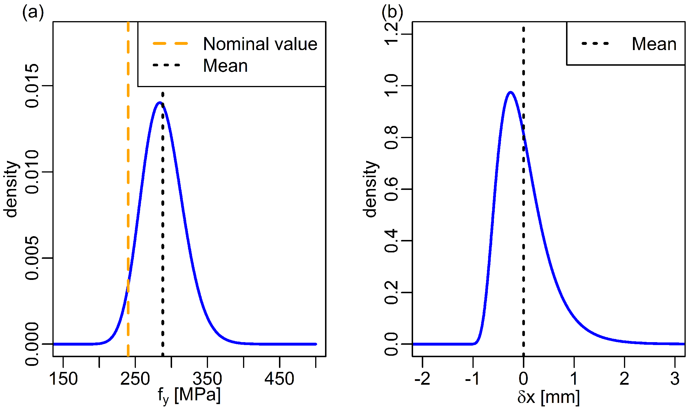
The yield strength of the steel for the two models studied has a nominal value of 240 MPa. In a probabilistic assessment, it is often modeled with a log-normal distribution [5,14,15]. We chose a mean of 1.2-times the nominal value and a coefficient of variation (COV) of 0.1, which results in the probability distribution shown in Figure 4a. Similarly, we model the manufacturing uncertainties (in units of mm) by another log-normal distribution, with a mean of 1.2 and COV of 0.5, shifted by 1.0 mm toward the right (Figure 4b). We propose this distribution here based on discussions with relevant industry. It is skewed toward the right, as manufacturers prefer to deliver more material than less, as this is considered conservative and therefore more acceptable to their clients.

Figure 4. Models for important sources of uncertainty. (a) Probability distribution of yield strength. Both the nominal value (orange) and the actual mean (black) are indicated. (b) Probability distribution of manufacturing uncertainties.

Figure 4. Models for important sources of uncertainty. (a) Probability distribution of yield strength. Both the nominal value (orange) and the actual mean (black) are indicated. (b) Probability distribution of manufacturing uncertainties.

The limit state function (Equation (5)) is evaluated with ${10}^5$ Monte Carlo samples from these two distributions, for each combination of loads considered, and these results are then transformed into a failure probability for the structural member in question. For this example, we did not correct for the probability of occurrence of the different load cases or the project lifetime, but simply report these numbers for each single 3-h load simulation, as a highly simplified estimate of the probability of failure due to a certain loading scenario. Variations in dimensions due to manufacturing uncertainty are also assumed not to change the stress resultants, in order to avoid performing additional, expensive load simulations for each sample. The effect of this approximation is assumed to be relatively minor compared to the changes in resistance due to the changing area and moments of inertia.

3. Results

3.1. Monopile

A typical result for the monopile is illustrated in Figure 5. The figure shows the axial force and total moment at the mudline for the OC3 monopile, as well as the value of the limit state function $g_2$ (Equation (5)). The load case is power production at rated wind speed under extreme turbulence. As expected, the maxima of forces and moments occur at different times. The Pareto front consists of 18 maximal pairs of values, indicated by the orange lines. Figure 6 shows the distribution of the values of the limit state function, for all values of the time series, for only the Pareto front (orange) and for the combination of the univariate maxima, as well as a scatterplot that illustrates that axial forces and bending moments seem to be more or less uncorrelated. Interestingly, the value of $g_2$ is completely dominated by the large bending moments (second term in Equation (5)), such that the values of $g_2$ for the univariate maxima and the worst value of $g_2$ for the Pareto front more or less coincide. In other words, in this case, the classical approach is well-suited and does not lead to an overtly conservative result.

Figure 5. Illustration of the difference between Pareto-optimal loads and the standard approach for the mudline location in the OC3 monopile, at rated wind speed (Design Load Case (DLC) 1.3). (a) Axial force; (b) total bending moment. The broken red lines indicate the locations and values of the univariate maxima. (c) Limit state function for combined bending and compression. The broken red line indicates the value for the conservative combination of univariate maxima. The dotted orange lines indicate the locations and values at the Pareto-optimal points. The nominal value of yield strength was used, and zero manufacturing uncertainty was assumed.

Figure 5. Illustration of the difference between Pareto-optimal loads and the standard approach for the mudline location in the OC3 monopile, at rated wind speed (Design Load Case (DLC) 1.3). (a) Axial force; (b) total bending moment. The broken red lines indicate the locations and values of the univariate maxima. (c) Limit state function for combined bending and compression. The broken red line indicates the value for the conservative combination of univariate maxima. The dotted orange lines indicate the locations and values at the Pareto-optimal points. The nominal value of yield strength was used, and zero manufacturing uncertainty was assumed.

Investigating the other load cases (Table 2), the situation remains similar. Differences in the values of the limit state function amount to less than half a percent. Apart from somewhat higher loads for the extreme turbulence model (DLC 1.3), there is not much difference with the operational load cases (DLC 1.1). In all cases, the approach using individual maxima is justified. As the design is obviously far from ultimate failure, the reliability analysis has been skipped for this structure.

Figure 6. Results for the mudline location in the OC3 monopile at rated wind speed (DLC 1.3). (a) The distribution of the limit state function evaluated at all points in time. The broken blue line indicates the value for the conservative combination of univariate maxima. The dotted orange lines indicate the values for the Pareto-optimal points. The solid line is an estimate of the underlying distribution, i.e., the theoretical case for an infinite number of samples. The actual samples from the time series are indicated with short black line segments at the bottom. (b) Scatter diagram showing axial force and bending moment. The Pareto-optimal front is indicated in orange. The single red point in the top right corner is the point obtained by the conservative approach.

Figure 6. Results for the mudline location in the OC3 monopile at rated wind speed (DLC 1.3). (a) The distribution of the limit state function evaluated at all points in time. The broken blue line indicates the value for the conservative combination of univariate maxima. The dotted orange lines indicate the values for the Pareto-optimal points. The solid line is an estimate of the underlying distribution, i.e., the theoretical case for an infinite number of samples. The actual samples from the time series are indicated with short black line segments at the bottom. (b) Scatter diagram showing axial force and bending moment. The Pareto-optimal front is indicated in orange. The single red point in the top right corner is the point obtained by the conservative approach.

Table 2. Results for the OC3 monopile, for the mudline location. Both power production under standard conditions (DLC 1.1) and extreme turbulence (DLC 1.3), as well as idling under extreme wind speeds (DLC 6.1) were assessed. The latter was investigated for two different values of the turbulence intensity (TI). Std: standard approach using univariate maxima; c$F_z$, c$M_{xy}$: contemporaneous maxima for $F_z$ or $M_{xy}$, respectively; PO: worst Pareto-optimal load vector. g: value of the limit state equation (Equation (5)).

Method	Parameters		DLC 1.1			DLC 6.1	DLC 1.3			DLC 6.1
	U	(m/s)	6	12	18	40.5	6	12	18	40.5
	TI	(%)	17.5	14.6	13.6	11.7	37.1	22.3	17.2	12.3
Std	$F_z$	(MN)	8.375	8.409	8.494	8.686	8.426	8.458	8.533	8.681
	$M_{xy}$	(MNm)	65.19	115.0	104.5	99.54	99.76	117.1	125.6	79.52
	g		0.791	0.658	0.686	0.699	0.699	0.653	0.630	0.752
c$F_z$	$F_z$	(MN)	8.375	8.409	8.494	8.686	8.426	8.458	8.533	8.681
	$M_{xy}$	(MNm)	20.72	75.04	26.79	29.22	76.56	87.26	42.50	29.67
	g		0.909	0.765	0.892	0.885	0.761	0.732	0.851	0.884
c$M_{xy}$	$F_z$	(MN)	8.359	8.308	8.299	8.509	8.377	8.319	8.282	8.511
	$M_{xy}$	(MNm)	65.19	115.0	104.5	99.54	99.76	117.1	125.5	79.52
	g		0.791	0.659	0.687	0.699	0.699	0.654	0.631	0.752
PO	$F_z$	(MN)	8.368	8.308	8.299	8.549	8.377	8.319	8.282	8.511
	$M_{xy}$	(MNm)	65.18	115.0	104.5	99.53	99.76	117.1	125.5	79.52
	g		0.791	0.659	0.687	0.699	0.699	0.654	0.631	0.752

Table 2. Results for the OC3 monopile, for the mudline location. Both power production under standard conditions (DLC 1.1) and extreme turbulence (DLC 1.3), as well as idling under extreme wind speeds (DLC 6.1) were assessed. The latter was investigated for two different values of the turbulence intensity (TI). Std: standard approach using univariate maxima; c$F_z$, c$M_{xy}$: contemporaneous maxima for $F_z$ or $M_{xy}$, respectively; PO: worst Pareto-optimal load vector. g: value of the limit state equation (Equation (5)).

Method	Parameters		DLC 1.1			DLC 6.1	DLC 1.3			DLC 6.1
	U	(m/s)	6	12	18	40.5	6	12	18	40.5
	TI	(%)	17.5	14.6	13.6	11.7	37.1	22.3	17.2	12.3
Std	$F_z$	(MN)	8.375	8.409	8.494	8.686	8.426	8.458	8.533	8.681
	$M_{xy}$	(MNm)	65.19	115.0	104.5	99.54	99.76	117.1	125.6	79.52
	g		0.791	0.658	0.686	0.699	0.699	0.653	0.630	0.752
c$F_z$	$F_z$	(MN)	8.375	8.409	8.494	8.686	8.426	8.458	8.533	8.681
	$M_{xy}$	(MNm)	20.72	75.04	26.79	29.22	76.56	87.26	42.50	29.67
	g		0.909	0.765	0.892	0.885	0.761	0.732	0.851	0.884
c$M_{xy}$	$F_z$	(MN)	8.359	8.308	8.299	8.509	8.377	8.319	8.282	8.511
	$M_{xy}$	(MNm)	65.19	115.0	104.5	99.54	99.76	117.1	125.5	79.52
	g		0.791	0.659	0.687	0.699	0.699	0.654	0.631	0.752
PO	$F_z$	(MN)	8.368	8.308	8.299	8.549	8.377	8.319	8.282	8.511
	$M_{xy}$	(MNm)	65.18	115.0	104.5	99.53	99.76	117.1	125.5	79.52
	g		0.791	0.659	0.687	0.699	0.699	0.654	0.631	0.752

3.2. Jacket Support Structure

For the jacket support structure, the loads have been assessed in a Y-joint at the bottom of the structure (location indicated in Figure 2). It has already been observed in Figure 1 that the situation for the brace at this joint is different from the monopile case: the values of $g_2$ for the Pareto-optimal points are much higher than the value for the univariate maxima. This is confirmed by looking at the distribution of these values (Figure 7). The scatterplot shows that there exists a certain pattern between axial force and bending moment, with a few extreme excursions defining the Pareto front. The latter indicates that the estimate of the probability of failure obtained from this time series is probably not very accurate, but this is an issue with the approach chosen in the IEC standard that goes beyond the scope of this article. More importantly, in this case, the contribution of axial force and bending moment in the limit state function is at a comparative level; therefore, the values of $g_2$ are significantly overpredicted by the standard approach, and our approach becomes justified.

Figure 7. Results for the bottom joint in the OC4 jacket support structure at rated wind speed (DLC 1.3). (a) The distribution of the limit state function evaluated at all points in time. The broken blue line indicates the value for the conservative combination of univariate maxima. The dotted orange lines indicate the values for the Pareto-optimal points. The solid line is an estimate of the underlying distribution, i.e., the theoretical case for an infinite number of samples. The actual samples from the time series are indicated with short black line segments at the bottom. (b) Scatter diagram showing axial force and bending moment. The Pareto-optimal front is indicated in orange. The single red point in the top right corner is the point obtained by the conservative approach. Note that, in contrast to Figure 1, the complete time series was used.

Figure 7. Results for the bottom joint in the OC4 jacket support structure at rated wind speed (DLC 1.3). (a) The distribution of the limit state function evaluated at all points in time. The broken blue line indicates the value for the conservative combination of univariate maxima. The dotted orange lines indicate the values for the Pareto-optimal points. The solid line is an estimate of the underlying distribution, i.e., the theoretical case for an infinite number of samples. The actual samples from the time series are indicated with short black line segments at the bottom. (b) Scatter diagram showing axial force and bending moment. The Pareto-optimal front is indicated in orange. The single red point in the top right corner is the point obtained by the conservative approach. Note that, in contrast to Figure 1, the complete time series was used.

This situation is basically unchanged across the different load cases (Table 3); only the degree of conservatism changes. The reliability assessment confirms the importance of using less conservative loads. The difference in loads is most pronounced for extreme wind speeds (DLC 6.1), where it can result in almost an order of magnitude difference in the probability of failure. Interestingly, the worst loading occurs around rated wind speed, where the member actually fails the ULS check (negative value of the limit state function).

The use of contemporaneous loads results in two values for $g_2$, one for the maximal axial force and one for the maximal bending moment. It depends on the load case which one is lower. Typically, the value for DLC 1.1 and DLC 1.3 is determined by the maximum bending moment (and the same-time axial force), whereas the value for DLC 6.1 is determined by the maximum of the axial force (and the same-time bending moment). The approach is non-conservative: the values of $g_2$ are larger than the ones obtained with the worst Pareto-optimal vector. This difference is most pronounced for the higher operational wind speed (18 m/s), where also almost an order of magnitude difference in the probability of failure was found (e.g., from 0.038–0.13 for DLC 1.3 or from 0.001–0.10 for DLC 1.1).

A result of the reliability analysis performed here is that manufacturing uncertainty does not seem to significantly influence the structural performance, compared to the dominating effect of the uncertainty in yield strength. This was somewhat unexpected, but is reassuring. Note, however, that only a limited analysis was performed here. Manufacturing uncertainty could well be relevant for other criteria and for local details that were not considered in this analysis.

Table 3. Results for the OC4 jacket, for the Y-joint at the bottom of the structure. Both power production under standard conditions (DLC 1.1) and extreme turbulence (DLC 1.3), as well as idling under extreme wind speeds (DLC 6.1) were assessed. The latter was investigated for two different values of the turbulence intensity (TI). Std: standard approach using univariate maxima; c$F_z$, c$M_{xy}$: contemporaneous maxima for $F_z$ or $M_{xy}$, respectively; PO: worst Pareto-optimal load vector; g: value of the limit state equation (Equation (5)); fail: failure probability, estimated by sampling random values from yield strength; fail*: additional sampling for manufacturing uncertainty. In contrast to Figure 1, these results are based on the full time series record.

Method	Parameters		DLC 1.1			DLC 6.1	DLC 1.3			DLC 6.1
	U	(m/s)	6	12	18	40.5	6	12	18	40.5
	TI	(%)	17.5	14.6	13.6	11.7	37.1	22.3	17.2	12.3
Std	$F_z$	(MN)	6.592	8.969	8.106	7.589	8.539	9.120	9.313	7.003
	$M_{xy}$	(MNm)	0.275	0.854	0.899	0.294	0.748	1.226	1.174	0.306
	g		0.247	−0.213	−0.146	0.142	−0.130	−0.374	−0.373	0.195
	fail		$<{10}^{-5}$	0.58	0.35	0.0003	0.29	0.94	0.93	$3\times {10}^{-5}$
	fail*		$<{10}^{-5}$	0.58	0.35	0.0004	0.29	0.94	0.93	$5\times {10}^{-5}$
c$F_z$	$F_z$	(MN)	6.592	8.969	8.106	7.589	8.539	9.120	9.313	7.003
	$M_{xy}$	(MNm)	0.158	0.577	0.160	0.191	0.673	0.266	0.232	0.131
	g		0.293	−0.104	0.144	0.183	−0.100	0.004	−0.002	0.264
	fail		$<{10}^{-5}$	0.22	0.0005	0.0001	0.21	0.035	0.038	$<{10}^{-5}$
	fail*		$<{10}^{-5}$	0.22	0.0004	0.0001	0.21	0.035	0.039	$<{10}^{-5}$
c$M_{xy}$	Fz	(MN)	6.323	8.128	5.428	2.484	8.375	8.447	4.960	5.577
	$M_{xy}$	(MNm)	0.275	0.854	0.899	0.294	0.748	1.226	1.174	0.306
	g		0.274	−0.131	0.116	0.642	−0.114	−0.308	0.053	0.334
	fail		$<{10}^{-5}$	0.30	0.001	$<{10}^{-5}$	0.24	0.84	0.011	$<{10}^{-5}$
	fail*		$<{10}^{-5}$	0.30	0.002	$<{10}^{-5}$	0.24	0.84	0.010	$<{10}^{-5}$
PO	$F_z$	(MN)	6.323	8.943	7.195	7.583	8.375	8.945	7.373	6.614
	$M_{xy}$	(MNm)	0.275	0.682	0.880	0.194	0.748	1.190	0.880	0.266
	g		0.274	−0.143	−0.050	0.182	−0.114	−0.343	−0.067	0.249
	fail		$<{10}^{-5}$	0.34	0.10	$5\times {10}^{-5}$	0.24	0.90	0.13	$<{10}^{-5}$
	fail*		$<{10}^{-5}$	0.33	0.10	$7\times {10}^{-5}$	0.24	0.90	0.13	$<{10}^{-5}$

Table 3. Results for the OC4 jacket, for the Y-joint at the bottom of the structure. Both power production under standard conditions (DLC 1.1) and extreme turbulence (DLC 1.3), as well as idling under extreme wind speeds (DLC 6.1) were assessed. The latter was investigated for two different values of the turbulence intensity (TI). Std: standard approach using univariate maxima; c$F_z$, c$M_{xy}$: contemporaneous maxima for $F_z$ or $M_{xy}$, respectively; PO: worst Pareto-optimal load vector; g: value of the limit state equation (Equation (5)); fail: failure probability, estimated by sampling random values from yield strength; fail*: additional sampling for manufacturing uncertainty. In contrast to Figure 1, these results are based on the full time series record.

Method	Parameters		DLC 1.1			DLC 6.1	DLC 1.3			DLC 6.1
	U	(m/s)	6	12	18	40.5	6	12	18	40.5
	TI	(%)	17.5	14.6	13.6	11.7	37.1	22.3	17.2	12.3
Std	$F_z$	(MN)	6.592	8.969	8.106	7.589	8.539	9.120	9.313	7.003
	$M_{xy}$	(MNm)	0.275	0.854	0.899	0.294	0.748	1.226	1.174	0.306
	g		0.247	−0.213	−0.146	0.142	−0.130	−0.374	−0.373	0.195
	fail		$<{10}^{-5}$	0.58	0.35	0.0003	0.29	0.94	0.93	$3\times {10}^{-5}$
	fail*		$<{10}^{-5}$	0.58	0.35	0.0004	0.29	0.94	0.93	$5\times {10}^{-5}$
c$F_z$	$F_z$	(MN)	6.592	8.969	8.106	7.589	8.539	9.120	9.313	7.003
	$M_{xy}$	(MNm)	0.158	0.577	0.160	0.191	0.673	0.266	0.232	0.131
	g		0.293	−0.104	0.144	0.183	−0.100	0.004	−0.002	0.264
	fail		$<{10}^{-5}$	0.22	0.0005	0.0001	0.21	0.035	0.038	$<{10}^{-5}$
	fail*		$<{10}^{-5}$	0.22	0.0004	0.0001	0.21	0.035	0.039	$<{10}^{-5}$
c$M_{xy}$	Fz	(MN)	6.323	8.128	5.428	2.484	8.375	8.447	4.960	5.577
	$M_{xy}$	(MNm)	0.275	0.854	0.899	0.294	0.748	1.226	1.174	0.306
	g		0.274	−0.131	0.116	0.642	−0.114	−0.308	0.053	0.334
	fail		$<{10}^{-5}$	0.30	0.001	$<{10}^{-5}$	0.24	0.84	0.011	$<{10}^{-5}$
	fail*		$<{10}^{-5}$	0.30	0.002	$<{10}^{-5}$	0.24	0.84	0.010	$<{10}^{-5}$
PO	$F_z$	(MN)	6.323	8.943	7.195	7.583	8.375	8.945	7.373	6.614
	$M_{xy}$	(MNm)	0.275	0.682	0.880	0.194	0.748	1.190	0.880	0.266
	g		0.274	−0.143	−0.050	0.182	−0.114	−0.343	−0.067	0.249
	fail		$<{10}^{-5}$	0.34	0.10	$5\times {10}^{-5}$	0.24	0.90	0.13	$<{10}^{-5}$
	fail*		$<{10}^{-5}$	0.33	0.10	$7\times {10}^{-5}$	0.24	0.90	0.13	$<{10}^{-5}$

4. Discussion

We have introduced the concept of Pareto-optimal loads as a tool for obtaining an efficient representation of extreme loads. The classical way of using univariate maxima is adequate in the case that one load component dominates all others. This is the case for the OC3 monopile, for example, where the bending moment more or less determines the value of the limit state equations. This also holds for the OC4 jacket at the larger elements, such as the tower bottom or mudline (results not shown). However, in the smaller structural details, such as the braces of the jacket, the contribution of the different load components in the limit state equation becomes more similar, and the use of univariate maxima is then very conservative. The recent edition of the IEC 61400-1 standard [4] introduced the concept of contemporaneous load vectors, in order to address this issue. However, it was found here that these lead to non-conservative results.

The example considered only two reference support structures. If designs are optimized, the likelihood increases that the univariate maxima are over-predicting the actual loads.

However, the main issue in favor of the proposed approach is structural reliability and reliability-based design optimization. Determining the probability of structural failure (due to extreme loads) accurately becomes very challenging and can only be performed for a small number of extreme loads. As seen in Section 2.2, the Pareto-optimal points are excellent candidates for this.

One advanced issue that we have neglected in this story so far is the statistical extrapolation of responses and loads. It is common practice to fit an extreme value distribution to the univariate extremes observed in simulations of operational load cases (DLC 1.1) and to predict a 50-year extreme response or load from this curve [16,17]. In detail, either block maxima (one value for each 10-min load case with a different random realization of wind and waves) or the exceedances over a high threshold are used [18]. This approach breaks down when multivariate extremes are considered, such as is the case here, and other methods, such as the inverse First Order Reliability Method (FORM), need to be used [19,20], with well-known limitations (such as being computationally much more involved). However, the method allows for consistently dealing with dynamic problems [21]. Using Pareto-optimal points for extrapolating multivariate extremes potentially offers an interesting alternative here, as well, but the details are left for future work.

5. Conclusions

The proposed method is easy to implement and use and can offer a significant advantage, both in the early design phases of a support structure, as well as during an assessment of structural reliability and probabilistic design. In the simple example case studied here, it effectively reduced the information contained in 144,000 time points into around 20 Pareto-optimal pairs of values that completely characterized the structure of the extreme loads, preserving in particular the non-trivial correlation between different load components.

For designs that are dominated by one load component, it is not necessary to consider the Pareto-optimal elements. Typical monopiles seem to fall into this category, as do larger members in jacket structures. However, both for smaller elements in jackets, as well as when performing structural optimization [22,23], it becomes important to evaluate the ULS condition with realistic loads. If this cannot be done for each time step simulated, such as in a computationally-involved reliability assessment, the Pareto-optimal points offer a safe and efficient alternative.

Other applications of the concept of Pareto-optimal vectors can be envisaged, as well. We already mentioned the accurate extrapolation of multivariate, correlated extremes for large return levels, but we also foresee applications in, e.g., condition monitoring of wind turbines.