Crisscross Optimization Algorithm and Monte Carlo Simulation for Solving Optimal Distributed Generation Allocation Problem

Abstract

Distributed generation (DG) systems are integral parts in future distribution networks. In this paper, a novel approach integrating crisscross optimization algorithm and Monte Carlo simulation (CSO-MCS) is implemented to solve the optimal DG allocation (ODGA) problem. The feature of applying CSO to address the ODGA problem lies in three interacting operators, namely horizontal crossover, vertical crossover and competitive operator. The horizontal crossover can search new solutions in a hypercube space with a larger probability while in the periphery of each hypercube with a decreasing probability. The vertical crossover can effectively facilitate those stagnant dimensions of a population to escape from premature convergence. The competitive operator allows the crisscross search to always maintain in a historical best position to quicken the converge rate. It is the combination of the double search strategies and competitive mechanism that enables CSO significant advantage in convergence speed and accuracy. Moreover, to deal with system uncertainties such as the output power of wind turbine and photovoltaic generators, an MCS-based method is adopted to solve the probabilistic power flow. The effectiveness of the CSO-MCS method is validated on the typical 33-bus and 69-bus test system, and results substantiate the suitability of CSO-MCS for multi-objective ODGA problem.

1. Introduction

In recent years, environmental concerns, fossil fuel resource depletion and advances in technology have resulted in the increase of distributed generation (DG) in distribution networks [1,2]. Reasonable application of DGs can bring many advantages, such as voltage profile improvement and pollutant emission reduction [3,4,5]. However, inappropriate allocation of DGs may also lead to voltage fluctuations and system instability due to the uncertain nature of renewable resources [6,7]. It is crucial to develop proper models and methodologies to identify the optimal allocation of DGs, the aim of which is to determine the best types, locations and sizes of DGs taking into account system uncertainties.

The optimal DG allocation (ODGA) problem in distribution networks has been investigated in the literature from different perspectives. In [8], an optimization model was proposed for optimizing DG allocation problem, but it mainly focused on total planning cost minimization. In [9], four indices including real and reactive power loss, voltage profile and feeder capacity were considered for the ODGA problem in distribution systems with different load models. The optimization model was more comprehensive, but the environmental benefits were not taken into account. An analytical approach was developed in [10] in order to determine the optimal location of DG to minimize the power loss of the system. However, the optimal sizes and types of DGs were not discussed. The authors in [11] applied Game Optimization Theory (GOT) and Distance Entropy Multi-Objective Particle Swarm Optimization (DEMPSO) algorithm to solve the multi-objective optimization problem. However, the issues relating to DG types and uncertain outputs of DGs were not involved in the work. Studies in [12,13,14,15] applied various algorithms such as PSO, Honey Bee Mating Optimization (HBMO) algorithm, two-layer Simulation-Based Optimization (SBO) and modified Fire Fly (MFF) algorithm to obtain the optimal allocation of DGs, but all of them were based on deterministic methods, which may not be consistent with the actual situations.

Although renewable energy source (RES) generators are essential elements in the future distribution networks, only a few papers have considered the stochastic nature of RES-based DGs in system planning. The authors in [16] proposed an improved adaptive genetic algorithm (IAGA) for solving the ODGA problem. The timing characteristics of DG outputs and loads as well as the environmental benefits are taken into account. The planning results considering uncertainties were more feasible in practical application. The authors in [17] developed a method that embedded genetic-algorithm with Monte Carlo simulation (GA-MCS) to solve the ODGA model under the uncertainties of RES generation and volatile fuel prices. However, only total cost of DGs and energy losses were taken into account in the model, the environmental benefits were not considered. Reference [18] proposed a multi-objective planning method based on GA considering system uncertainties. However, only the wind-based and photovoltaic-based DG units were considered, and the GA solution method has some shortcomings like premature and slow convergence, which may lose the best solution. In [19], a novel method based on Cuckoo Search (CS) algorithm was proposed for low-carbon active distribution system planning. The uncertainties of renewable energy had been considered through scenario synthesis method. However, only the wind-based DGs were considered, and other kinds of DGs like photovoltaic generators and micro-gas turbines were not taken into account.

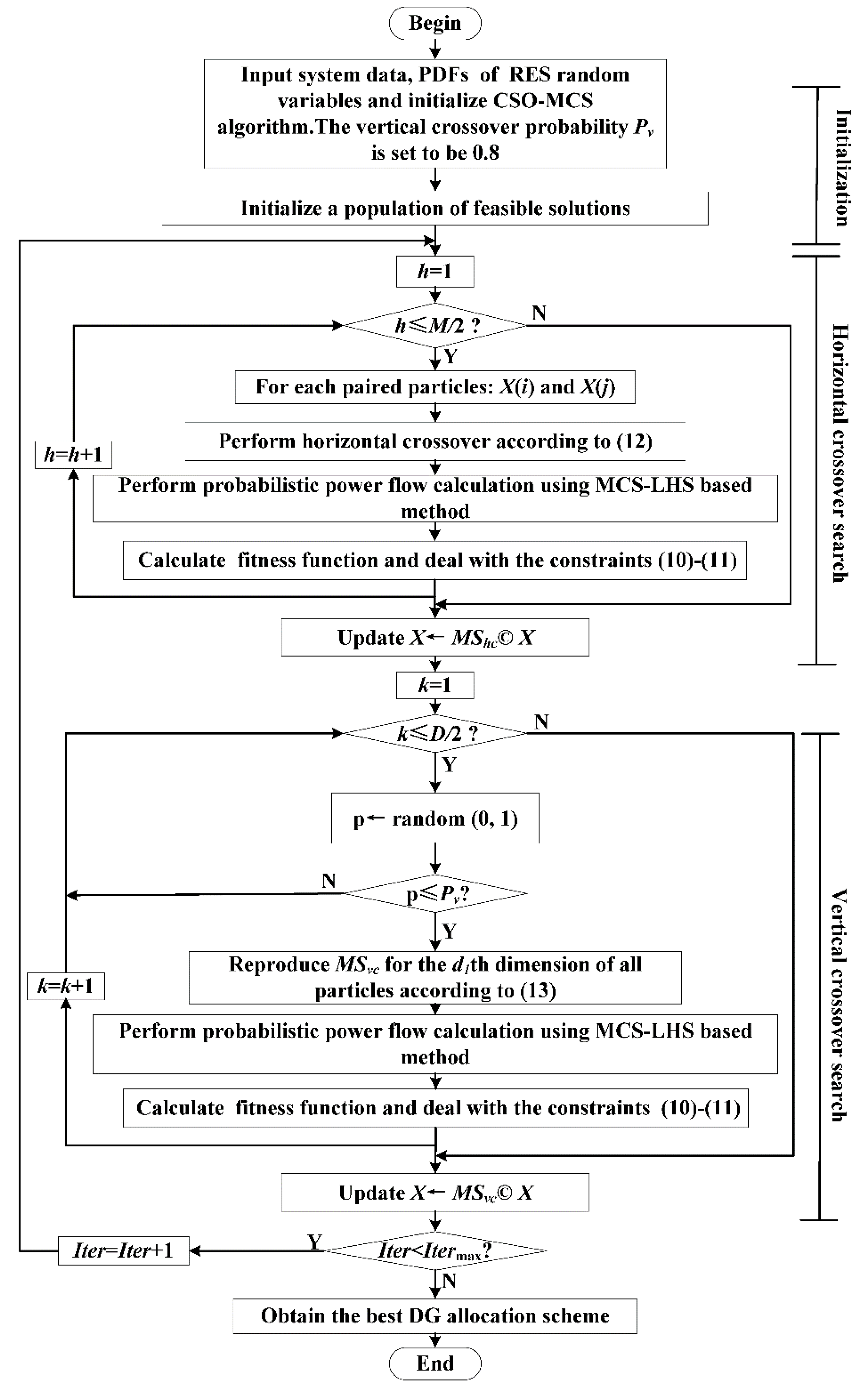
In this paper, we propose a novel approach integrating crisscross optimization algorithm and Monte Carlo simulation (CSO-MCS) for solving the ODGA problem. The crisscross optimization (CSO) algorithm is a recent evolutionary algorithm inspired by Confucian doctrine of gold mean and the crossover operation of genetic algorithm. Compared to other population-based algorithms, it offers lower computational burden and higher convergence speed when solving complex optimization problems. In this study, we firstly attempt to apply the CSO algorithm to solve the complex ODGA problem with technical benefits, economical benefits and environmental benefits taken into account. Meanwhile, to deal with the system uncertainties which have great influence on the DG planning results, an MCS-based method is adopted to solve the probabilistic power flow (PPF). Furthermore, we establish a multi-objective ODGA model based on a chance constrained programming (CCP) framework, aiming to determine the best types, locations and sizes of DGs in the distribution system. The pollutant emission cost, the total DG cost and the power loss costs are used to develop the objective functions. All these costs are represented by their net present values (NPV), which are compounded over the planning period of DGs. Three types of DGs including wind turbine (WT), photovoltaic (PV) generators and micro-gas turbines (MT) are considered in the ODGA problem.

The main contribution of this paper is to develop the CSO-MCS method to the ODGA problem considering system uncertainties of wind, solar and load consumption. The reminder of this paper is organized as follows: Section 2 and Section 3 present the modeling of system uncertainties and the ODGA model under CCP framework. Section 4 introduces the proposed CSO-MCS solution strategy, and Section 5 presents the results and discussion, followed by the conclusions in the last section.

2. Modeling of Uncertainties

2.1. Modeling of Wind Turbines (WT) Generation

Many experiments have demonstrated that the stochastic behavior of wind speed in most regions approximately follows the Weibull distribution [17]; the probability density function (PDF) of wind speed v can be expressed as:

$$f(v)=\frac{k}{c}{(\frac{v}{c})}^{k-1}\text{exp}[-{(\frac{v}{c})}^k]$$

(1)

where k and c are the shape index and the scale index of Weibull distribution.

The output power of wind turbines varies with the wind speed, and its models can be formulated as:

$$P_{WT}=\{\begin{array}{l}0,v\le v_{ci},v\ge v_{co}\\ P_{WT\_n}\frac{v-v_{ci}}{v_n-v_{ci}},v_{ci}\le v\le v_n\\ P_{WT\_n},v_n\le v\le v_{co}\end{array}$$

(2)

where P_{WT_n} is rated power; v is the wind speed; v_ci, v_co and v_n are the cut-in wind speed, cut-out wind speed and rated wind speed.

2.2. Modeling of Photovoltaic (PV) Generation

The solar illumination intensity is considered as the dominant factor affecting the PV output power, and it approximately follows the Beta distribution with a PDF as Equation (3) [20]:

$$f(r)=\frac{\mathsf{\Gamma }(\mathsf{\alpha }+\mathsf{\beta })}{\mathsf{\Gamma }(\mathsf{\alpha })\mathsf{\Gamma }(\mathsf{\beta })}{(\frac{r(t)}{r_{\text{max}}})}^{\mathsf{\alpha }-1}{(1-\frac{r(t)}{r_{\text{max}}})}^{\mathsf{\beta }-1}$$

(3)

where r_max represents the maximum intensity of sunlight in a certain period of time; and α and β are the shape parameters of the Beta distribution, respectively.

The output power of PV is related to the solar illumination intensity, their relationship can be described as:

$$P_s(t)=P_{stc}\frac{r(t)}{r_{stc}}[1+k(T(t)-T_{stc})]$$

(4)

where P_s(t) is the output power of photovoltaic under illumination intensity t; T(t) is the surface temperature of the photovoltaic array; r_stc, T_stc and P_stc are the intensity of sunlight, the surface temperature of the photovoltaic array and the maximum output power in the standard testing environment (1 kW/m²), 25 °C; k is the temperature coefficient.

2.3. Modeling of Load Data

The load P_L is assumed to be a random variable that follows the normal distribution [17]. The probability density function of P_L is given by the following expression:

$$f(P_L)=\frac{1}{\sqrt{2\mathsf{\pi }}{\mathsf{\sigma }}_P}\text{exp}[-\frac{{(P_L-{\mathsf{\mu }}_P)}^2}{2{\mathsf{\sigma }}_P^2}]$$

(5)

where μ_P is the mean value; and σ_P is the standard deviation.

3. Formulation of the ODGA Problem

A multi-objective ODGA model considering environmental benefit, total DG cost and power loss is established under the chance constrained programming (CCP) framework. In this section, the objective functions and constraints are explained.

3.1. Pollutant Emissions

DG allocation problem considering environmental benefits can achieve the best balance between economic and environmental benefits. The pollutant emissions of the distribution system mainly consist of two parts, namely, the pollutant emissions from thermal power units and the pollutant emissions from of DG units. An environmental cost index is given as follows:

$$f_1=C_{ems}={\displaystyle \sum _{b=1}^T}{(\frac{1}{1+\mathsf{\eta }})}^b[({\displaystyle \sum _{n=1}^{N_{DG}}}{S}_{DG,n}\times {pf}_{DG,n}\times T_{DG,n}+{\displaystyle \sum _{k=1}^{N_{sub}}}{P}_{sub,n}\times T_{sub,n})\times {\displaystyle \sum _{i=1}^K}{Q}_{n,i}(V_{n,i}+{PN}_{n,i})]$$

(6)

where 1/(1+η)^b represents the present value of the annual cost considering discount rate η in the bth year; T is the total number of DG planning years; S_DG,n and pf_DG,n are the installed capacity and power factor of the nth DG; P_sub,n is the power of nth thermal power unit; T_DG,n and T_sub,n are the equivalent generation hours of DG and thermal power generation in one year; N_DG and N_sub are the total number of DGs and substations in the distribution network; Q_n,i is the amount of the ith pollutant emissions from the nth generator per active power (kg/kWh); and V_n,i and PN_n,i are the environmental treatment cost and penalty fee of the ith pollutant ($/kg), respectively [21]; K is the types of pollutant.

3.2. Total DG Cost

The total DG cost factor including the investment cost $C_{DG}^I$, operating and maintenance (O&M) cost $C_{DG}^{OM}$ along the planning period is formulated as the expression given in Equation (7).

$$f_2=C_{DG}=C_{DG}^I+C_{DG}^{OM}={\displaystyle \sum _{b=1}^T}{(\frac{1}{1+\mathsf{\eta }})}^b\left[{\displaystyle \sum _{i=1}^{N_{DG}}}{\displaystyle \sum _{k=1}^{N_{type}}}(C_{DGk}^I{P}_{DGik}+C_{DGk}^{OM}{T}_{DGik}{P}_{DGik})\right]$$

(7)

where $C_{DGk}^I$ and $C_{DGk}^{OM}$ are the per-unit investment cost and operation and maintenance cost of the kth type of DG, respectively; P_DGik is the installed capacity of the kth type of DG in candidate location i; T_DGik is the equivalent generation hours of the kth type of DG in candidate location i in one year; N_DG is the set of candidate buses for installing DG; N_type is the number of types of DGs.

Due to the uncertain output power of renewable DGs, it is not an easy task to accurately evaluate the O&M costs. In this paper, the O&M costs are equivalent to the cost for per unit of electricity generated (i.e., $/kWh) as [22] and [23] did.

3.3. System Power Losses

This objective is to minimize the system power losses of distribution network. The power losses cost can be expressed as follows:

$$f_3=C_{ploss}={\displaystyle \sum _{b=1}^T}{(\frac{1}{1+\mathsf{\eta }})}^b\left[p_r\times T_{\text{max}}{\displaystyle \sum _{n=1}^{N_{branch}}}{I}_n^2{R}_n\right]$$

(8)

where, p_r is the electricity price; T_max is the equivalent time of load consumption (i.e., annual maximum load utilization hours), which expression can refer to [24]; I_n is the current corresponding to the annual maximum load utilization hours of the nth branch; R_n is the resistance of the nth branch; N_branch is the number of branches.

3.4. Objective Function

The cost of ODGA problem is considered in one unique objective function that formulated as below:

$$\text{min} F=\mathsf{\mu }{C}_{ems}+\mathsf{\lambda }{C}_{DG}+\mathsf{\xi }{C}_{loss}$$

(9)

where C_ems is the environmental cost; C_DG is the total DG cost; C_loss is the power losses cost; and μ, λ and ξ are weighting coefficients for each sub objective.

Due to the multi-objective feature of Equation (9), a method named analytic hierarchy process (AHP) is employed to determine the weighting coefficients as [17] did. The AHP method was first proposed by T. Saaty in 1970, and now it has gradually become an algorithm with extensive applications in multi-objective comprehensive evaluations [17]. When determining the weight coefficients, experts from related fields should be invited to score for sub objectives, and then the weight coefficients can be by the AHP method.

In some developing countries, DG technologies are still in the primary stage of development. Because of the immature technology, high costs or specific power market system, either the social investors or private investors have high barriers to participate in the field of DG at present or even some time in the future. Therefore, in this paper, proceeding from the realities in some developing countries, we studied the optimization problem from the view point of power grid companies. However, the established ODGA model can also be used for other stockholders through adjusting the weight coefficients of the three sub objectives in Equation (9) using the AHP method.

3.5. Constraints

3.5.1. Deterministic Constraints

The deterministic constraints are the load-flow equations and the DG capacity constraints that showed in Equation (10).

$$\{\begin{array}{l}{P}_{Gi}-P_{Li}=V_i{\displaystyle \sum _{k\in A(i)}}{V}_k(G_{ik} \text{cos}{\mathsf{\delta }}_{ik}+B_{ik} \text{sin}{\mathsf{\delta }}_{ik})\\ Q_{Gi}-Q_{Li}=V_i{\displaystyle \sum _{k\in A(i)}}{V}_k(G_{ik} \text{sin}{\mathsf{\delta }}_{ik}-B_{ik} \text{cos}{\mathsf{\delta }}_{ik})\\ P_{DGi\text{min}}\le P_{DGi}\le P_{DGi\text{max}}\\ Q_{DGi\text{min}}\le Q_{DGi}\le Q_{DGi\text{max}}\\ {\displaystyle \sum _{i=1}^{N_{DG}}}{P}_{DGi}\le {PEN}_{\text{max}}{\displaystyle \sum _{i=1}^{N_{bus}}}{P}_{Li}\end{array}$$

(10)

where P_Gi and Q_Gi are the active and reactive output power of the generators at node i; P_Li and Q_Li are the active and reactive load power at node i; V_i and V_k are the voltage amplitudes at node i and node k; G_ik and B_ik are the conductance and susceptance between node i and node k; δ_ik is the voltage angle between node i and node k. P_DGimax and P_DGimin are the upper and lower limits of active output power of DGs; Q_DGimax and Q_DGimin are the upper and lower limits of reactive output power of DGs. P_Li is the active load power at node i, PEN_max is the maximum allowable penetration of DG; and N_DG and N_bus are the number of installed DGs and buses of network, respectively.

3.5.2. Chance Constraints

Chance constraint programming (CCP) is a stochastic programming method that suitable for solving optimization problem with uncertainties. More details about CCP can refer to [17,25]. In the CCP optimization framework, some constraints are allowed to be satisfied within a certain confidence level when uncertain nature of renewable DGs are considered. The chance constraints of node voltage and the permissible power flow in this work are given as:

$$\{\begin{array}{l}\mathrm{Pr}\{V_{\text{min}}\le V_i\le V_{\text{max}}\}\ge \mathsf{\alpha }\\ \mathrm{Pr}\{S_{ij}\le S_{ij\text{max}}\}\ge \mathsf{\beta }\end{array}$$

(11)

where, α and β are the confidence level of permissible voltage and power flow under the CCP framework. V_min and V_max are the the upper and lower limits of voltage amplitude; S_ij and S_ijmax are the power flow and the permitted maximal power flow limit in the feeder between node i and node j, respectively.

4. Proposed CSO-MCS Solution Approach

In this paper, an approach that embedded crisscross optimization algorithm with Monte Carlo simulation (CSO-MCS) is developed to find the best solution for the ODGA problem under uncertainties. In the solution approach, the CSO algorithm is dedicated to search the best solution among a number of feasible solutions, and the MCS-based probabilistic power flow (PPF) method is used to deal with the system uncertainties and solve the power flow.

4.1. Determination of Feasible Solutions Using CSO

The crisscross optimization algorithm (CSO) is a recent evolutionary algorithm inspired by Confucian doctrine of gold mean and the crossover operation of genetic algorithm [26]. Compared to other heuristic algorithms, the CSO algorithm has a huge advantage in solution accuracy and convergence speed when addressing complex optimization problems [26,27]. The CSO algorithm is mainly made of three components: the horizontal crossover, the vertical crossover and the competitive operator. The horizontal crossover and vertical crossover execute within each iteration and reproduce their offspring solutions called moderation solutions by performing different crossover operations. Meanwhile, after each crossover operation, the competitive operator should be carried out to choose the better particle. Only those new solutions that outperform their parent particles can survive while the others will be eliminated in the competition. It is the combination of the double search strategies and competitive mechanism that enables CSO significant advantages in convergence speed and solution accuracy. The detailed introduction of the three components is described in the following subsections.

4.1.1. Horizontal Crossover

The horizontal crossover is used to generate the moderation solutions by executing a special arithmetic crossover operation on all the dimensions between two different particles so as to enlarge searching scopes. Suppose the ith parent particle X(i) and the jth parent particle X(j) are chosen to perform the horizontal crossover operation at the dth dimension, their offspring, namely the moderation solution, can be reproduced through the equations as shown in Equation (12).

$$\{\begin{array}{l}M{S}_{hc}(i,d)=r_1\times X(i,d)+(1-r_1)\times X(j,d)+c_1\times (X(i,d)-X(j,d))\\ M{S}_{hc}(j,d)=r_2\times X(j,d)+(1-r_2)\times X(i,d)+c_2\times (X(j,d)-X(i,d))\end{array}$$

(12)

where X(i,d) and X(j,d) are the dth dimension of two parent particle X(i) and X(j); r₁ and r₂ are random values uniformly distributed between 0 and 1; c₁ and c₂ are expansion coefficients uniformly distributed between −1 and 1; MS_hc(i,d) and MS_hc(j,d) are the offspring of X(i,d) and X(j,d), respectively.

In the process of the horizontal crossover, all particles of CSO are randomly divided into M/2 pairs. Each pair of particles reproduces two moderation solutions according to Equation (12). Through the horizontal crossover operator, new solutions can be searched in a hypercube space with a larger probability while in the periphery of each hypercube with a decreasing probability, which had been proved in [26]. This search mechanism gifts CSO with powerful global search ability. After horizontal crossover search, the moderation solutions should compete with their corresponding parent particles. The winners will save in the updated population and serve as the parent population of vertical crossover.

4.1.2. Vertical Crossover

The vertical crossover search is an arithmetic crossover operated on all the particles between two different dimensions. Suppose the d₁th and d₂th dimensions of the particle i (i.e., X(i,d₁) and X(i,d₂)) are used to carry out the vertical crossover operation, the d₁th dimension offspring of particle i (i.e., MS_vc(i,d₁)) can be reproduced by Equation (13).

$$M{S}_{vc}(i,d_1)=r\times X(i,d_1)+(1-r)\times X(i,d_2),i\in N(1,M),d_1,d_2\in N(1,D)$$

(13)

where r is a uniformly distributed random value between 0 and 1; M is the population size; D is the number of dimensions.

In the process of vertical crossover, all particles are randomly divided into D/2 pairs. The role of vertical crossover search is to facilitate some stagnant dimensions of the population and escape from dimension premature convergence. Unlike horizontal crossover, only a few paired dimensions are chosen to perform the vertical crossover operation because that about 10%–40% of the dimensions in the swarm may be simultaneously trapped into stagnancy when optimizing the multimodal functions [26]. Therefore, the vertical crossover probability P_vc is suggested to be set in the range [0.2, 0.8] in [26]. Similar to the horizontal crossover search, the new solutions should compete with the parent particle and those solutions that outperform their competitor can survive.

4.1.3. Competitive Operator

In CSO, a greedy selection strategy that is similar to the differential evolutionary algorithm is used to update the population, as expressed in Equation (14).

$$X\leftarrow MS\copyright X$$

(14)

Every time when the crossover operation is finished, the competitive operator need to be executed to choose the particle that has better fitness value. Only those moderation solutions that outperform their parent particles can survive, while all the rest are eliminated in the competition. Such competitive method allows the crisscross search always maintain in a historical best position and quicken the converge rate to the global optima.

4.1.4. Basic Procedure of CSO Algorithm

The basic procedure of CSO algorithm is given as follows:

Step 1.

Population initialization and parameters set.

Step 2.

Execute horizontal crossover with the competitive operator.

Step 3.

Execute vertical crossover with the competitive operator.

Step 4.

Repeat Steps 2 and 3 until the number of iterations is larger than the specified maximum value.

4.2. MCS-Based Probabilistic Power Flow Calculation

As mentioned before, ODGA problem becomes more complex when system uncertainties are considered. In order to obtain more feasible planning results, probabilistic power flow (PPF) calculation methods must be employed. Compared to the deterministic power flow, the PPF method characterizes the uncertainty in system information by describing the variation in terms of a suitable probability distribution. In this paper, the Monte Carlo simulations (MCS)-based PPF method proposed in [28] is adopted. The MCS is used to produce a large number of random variables according to the statistical models that established in Section 2. In case of uncertainties in the input variables of the power system, it is desirable to assess the system output variables (bus voltages and line flows) for many load and generation conditions. It is necessary to run the deterministic power flow routine many times in order to evaluate possible system states. More detailed principles about MCS-based probabilistic power flow method can refer to [28] and [29].The flowchart of MCS-based PPF method is shown in Figure 1.

Figure 1. Flowchart of MCS-based PPF calculation.

Figure 1. Flowchart of MCS-based PPF calculation.

4.3. Solving Steps of the CSO-MCS Method to ODGA Problem

The flowchart of the CSO-MCS algorithm is illustrated in Figure 2 and its procedure for solving ODGA problem can be described as follows:

Step 1:

Define the input data, including the network data and the specified parameters of CSO-MCS algorithm;

Step 2:

Randomly generate the initial population as showed in Equation (15).

$$Population=\left[\begin{array}{ccc}{P}_{11}^w\cdots P_{1N_w}^w,& P_{11}^p\cdots P_{1N_p}^p,& P_{11}^m\cdots P_{1N_m}^m\\ P_{21}^w\cdots P_{2N_w}^w,& P_{21}^p\cdots P_{2N_p}^p,& P_{21}^m\cdots P_{2N_m}^m\\ ⋮& ⋮& ⋮\\ P_{M1}^w\cdots P_{M{N}_w}^w,& P_{M1}^p\cdots P_{M{N}_p}^p,& P_{M1}^m\cdots P_{M{N}_m}^m\end{array}\right]$$

(15)

where $P_{ni}^w$, $P_{nj}^p$ and $P_{nk}^m$ (i = 1,2,...,N_w, j = 1,2,...,N_p, k = 1,2,...,N_m, n = 1,2,...,M) are the installation capacity of the ith WT unit, jth PV unit and kth MT unit, respectively. N_w, N_p and N_m are the number of candidate locations for WT, PV and MT. The initial population is filled with M randomly generated solutions.

Figure 2. Flowchart of CSO-MCS for solving the ODGA problem.

Figure 2. Flowchart of CSO-MCS for solving the ODGA problem.

Step 3:

Execute the MCS-based PPF calculation and check the feasibilities of CSO particles.

Step 4:

Calculate the fitness function of CSO particle according to Equations (6)–(9), using the results of the PPF.

Step 5:

Check the constraints of ODGA model with the results of the PPF. If the constraints are satisfied, go to the next step; otherwise, add a large value M_p to the fitness value as a penalty. Repeat Steps 3 to 5 for all particles of the initial population;

Step 6:

Sort the particles in descending order of fitness value and save current best solutions in the repository G_best;

Step 7:

Update the population using horizontal crossover and vertical crossover.

Step 8:

Repeat Steps 3–7 until predetermined iteration number is reached.

Step 9:

Select the best solution found in the above solving procedure as the best DG allocation scheme.

5. Numerical Results

To comprehensively demonstrate the validity of the proposed CSO-MCS algorithm, simulation studies are conducted on two test systems which are widely used as benchmarks in the power system planning field for solving the ODGA problems. The two test systems are the 33-bus and 69-bus distribution systems, respectively. The first 33-bus system is a radial system with total load of 3.715 MW. The second 69-bus system is a widely used distribution system in the literature. The detailed data of the systems appear in [30] and [31].

The parameters of the proposed model are specified as follows: (1) The planning period of DG is 15 years; the discount rate is 12%; (2) The voltage magnitude cannot exceed ±5% of the nominal voltage and the power flow on the lines should not exceed 4 MVA with the confidence levels of 90% (i.e., α = β = 0.9); (3) Weighting coefficients of Equation (9): μ = 0.2, λ = 0.38, ξ = 0.42. The electricity price is 0.089 $/kWh. The investment cost, operation, and maintenance cost and other technical parameters of WT/PV/MT generators can be seen in Table 1. In a practical situation, it cannot be expected that the O&M cost and electricity price always keep constant along the time. However, in order to simplify the problem, it is assumed that the O&M costs and the electricity price are as constant in the simulations.

Table 1. Technical specification parameters of different types of distributed generation (DGs).

DG type	Investment cost ($/kVA)	O&M cost ($/kWh)	Technical specification	Power factor
WT	1882	0.01	vio = 4 m/s, vco = 20 m/s, vn = 15 m/s	0.95 lagging
PV	4004	0.01	Pstc = 1000 W/m2	1.0
MT	2293	0.012	Stable power	0.9 lagging

Table 1. Technical specification parameters of different types of distributed generation (DGs).

DG type	Investment cost ($/kVA)	O&M cost ($/kWh)	Technical specification	Power factor
WT	1882	0.01	vio = 4 m/s, vco = 20 m/s, vn = 15 m/s	0.95 lagging
PV	4004	0.01	Pstc = 1000 W/m2	1.0
MT	2293	0.012	Stable power	0.9 lagging

The pollutant emission rates (kg/MWh) of different kinds of DGs are given in Table 2. The environmental value standard and penalty for pollutant emissions are shown in Table 3. When planning DG, a series of candidate places that suitable for installing specific types of DGs will be given, from the aspects of climate, geography and technology conditions. Then, the CSO-MCS will be used to determine the best schemes (i.e., the best types, locations and sizes of DGs) among the given candidate locations taking into account the voltage amplitude, power flow and total costs of the distribution system. It is assumed that the candidate types and locations of DGs in the 33-bus and 69-bus systems are as shown in Table 7 and Table 8, respectively; the size of the each DG unit is within the limit between 10 and 500 kVA with discrete interval capacity of 10 kVA.

Table 2. Pollutant emission rate of different types of DGs.

Generation type	Emission rate(kg/MWh)
	NOx	CO2	SO2
WT	0	0	0
PV	0	0	0
MT	0.52	502.6	3628.7
Grid	2.29	921.5	3.58

Table 2. Pollutant emission rate of different types of DGs.

Generation type	Emission rate(kg/MWh)
	NOx	CO2	SO2
WT	0	0	0
PV	0	0	0
MT	0.52	502.6	3628.7
Grid	2.29	921.5	3.58

Table 3. Environmental value standard and penalty for pollutant emissions.

Index	NOx	CO2	SO2
Environmental value ($/kg)	1.00	0.002875	0.75
Penalty ($/kg)	0.25	0.00125	0.125

Table 3. Environmental value standard and penalty for pollutant emissions.

Index	NOx	CO2	SO2
Environmental value ($/kg)	1.00	0.002875	0.75
Penalty ($/kg)	0.25	0.00125	0.125

To find the effectiveness and improvement of the developed CSO-MCS algorithm, the test results are compared with those obtained by another algorithm named PSO-MCS in [32]. All the experiments are implemented using Matlab2009b at a Core2 2.40-GHz machine with 2-GB RAM. The parameters of the algorithms are set as follows: In CSO-MCS, the horizontal crossover probability and vertical crossover probability are set as P_hc = 1 and P_vc = 0.8 according to the suggestion in [26]. In PSO-MCS, the acceleration coefficients are set to c₁ = c₂ = 0.8, the inertia weight is set to w = 0.4 [32]. In the two algorithms, the population sizes are set to N_pop = 50, the maximum number of iterations is set to Iter_max = 500, the sample sizes of Monte Carlo are set to N_s = 500, other parameters are set to the same as those used in the optimization model. To reduce statistical errors, the test is repeated 30 times independently.

5.1. Case 1: IEEE 33-Bus System

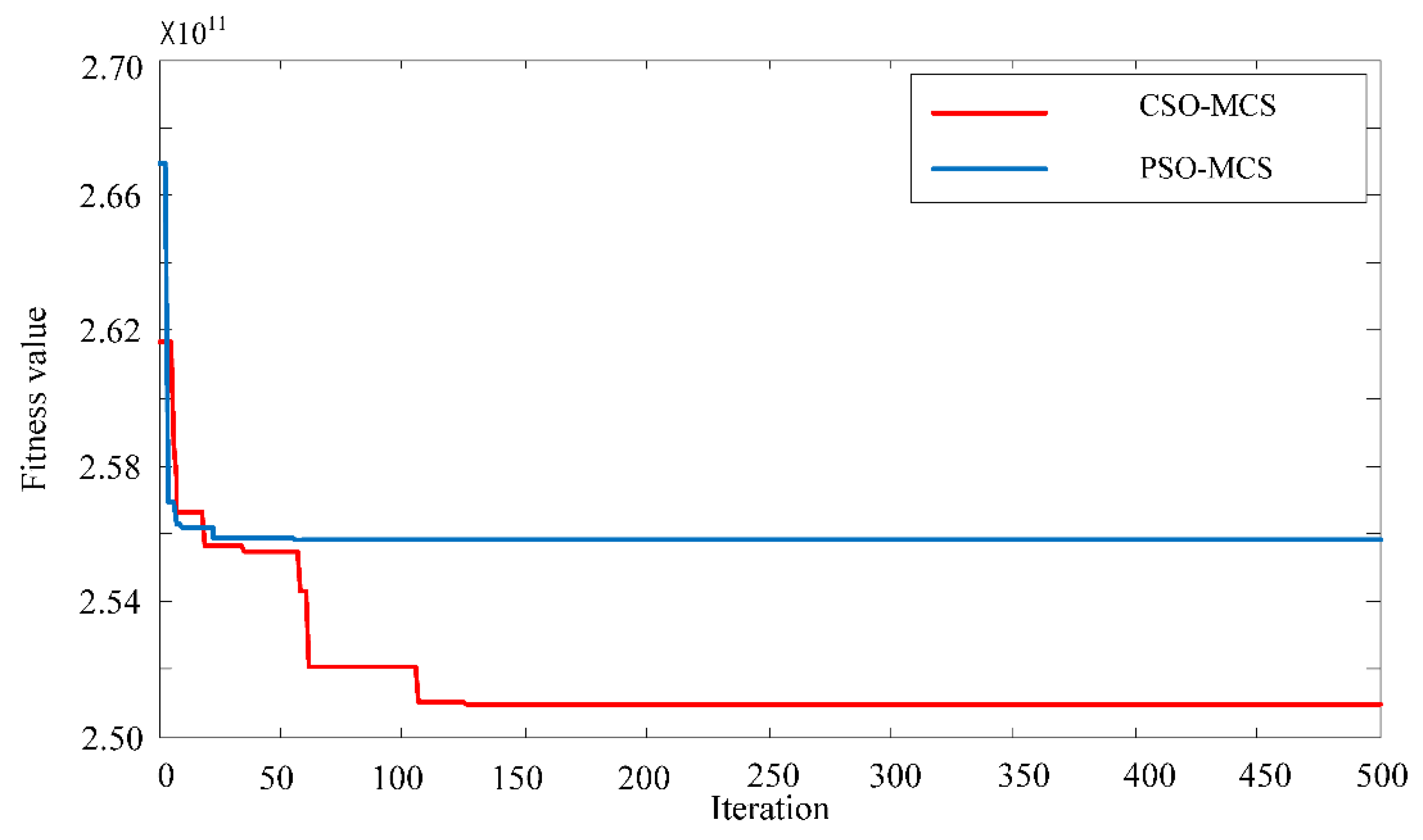
In this case, the typical 33-bus system is used to test the proposed method. The convergence characteristics of the developed CSO-MCS algorithm and PSO-MCS are illustrated in Figure 3. From this figure, it can be seen that the PSO-MCS algorithm is fast in convergence. The iteration number required by PSO-MCS is only 57. However, the convergence accuracy is not entirely satisfactory. This is due to the shortcoming of PSO that is easily trapped in the local optimum and appeared premature convergence. As to CSO-MCS, the experimental results show that its iteration number is greater than PSO-MCS, while the optimal result of CSO-MCS is 1.88% better than that of PSO-MCS.

Figure 3. Convergence characteristics of CSO-MCS and PSO-MCS (Case 1).

Figure 3. Convergence characteristics of CSO-MCS and PSO-MCS (Case 1).

The simulation results including the pollutant emissions, the power losses cost, the total DG cost and the CPU time obtained by CSO-MCS and the compared algorithm are shown in Table 4. The comparisons of statistics of the above indices, such as mean value, standard deviation, maximum and minimum value are presented as well. In terms of solution quality, we see that the mean pollutant emissions and power losses cost achieved by CSO-MCS is 25.08% and 14.40% less than those by PSO-MCS. The best fitness value CSO-MCS achieved is better than PSO-MCS as analyzed earlier.

These results demonstrate the effectiveness of the developed CSO-MCS algorithm in addressing DG allocation problems. With respect to the computing time, the mean CPU time of CSO-MCS is 227.02 s, which is 24.65% faster than PSO-MCS. In stability, we can see that the standard deviation of CPU time of CSO-MCS is 6.42 s, which is 47.38% less than PSO-MCS. Similar results can be found in other indices. For example, the standard deviation value of emissions index obtained by CSO-MCS is 68.89% less than that of PSO-MCS. These results show that CSO-MCS has good performance in robustness.

Table 4. Results obtained by crisscross optimization algorithm and Monte Carlo simulation (CSO-MCS) and particle swarm optimization and Monte Carlo simulation (PSO-MCS) (30 runs for Case 1).

Evaluation method		Pollutant emissions (105 t)	Power losses cost (105 $)	Total DG cost (106 $)	CPU time (s)
CSO-MCS	Maximum value	1.0695	5.5983	3.8402	239.72
	Minimum value	1.0599	5.1482	3.8367	215.34
	Mean	1.0651	5.4601	3.8387	227.02
	Standard deviation	0.0028	0.0417	0.000975	6.42
PSO-MCS	Maximum value	1.1152	6.1232	3.6945	350.64
	Minimum value	1.0802	6.4685	3.6448	295.75
	Mean	1.0925	6.3787	3.6716	301.27
	Standard deviation	0.0090	0.0743	0.0157	12.20

Table 4. Results obtained by crisscross optimization algorithm and Monte Carlo simulation (CSO-MCS) and particle swarm optimization and Monte Carlo simulation (PSO-MCS) (30 runs for Case 1).

Evaluation method		Pollutant emissions (105 t)	Power losses cost (105 $)	Total DG cost (106 $)	CPU time (s)
CSO-MCS	Maximum value	1.0695	5.5983	3.8402	239.72
	Minimum value	1.0599	5.1482	3.8367	215.34
	Mean	1.0651	5.4601	3.8387	227.02
	Standard deviation	0.0028	0.0417	0.000975	6.42
PSO-MCS	Maximum value	1.1152	6.1232	3.6945	350.64
	Minimum value	1.0802	6.4685	3.6448	295.75
	Mean	1.0925	6.3787	3.6716	301.27
	Standard deviation	0.0090	0.0743	0.0157	12.20

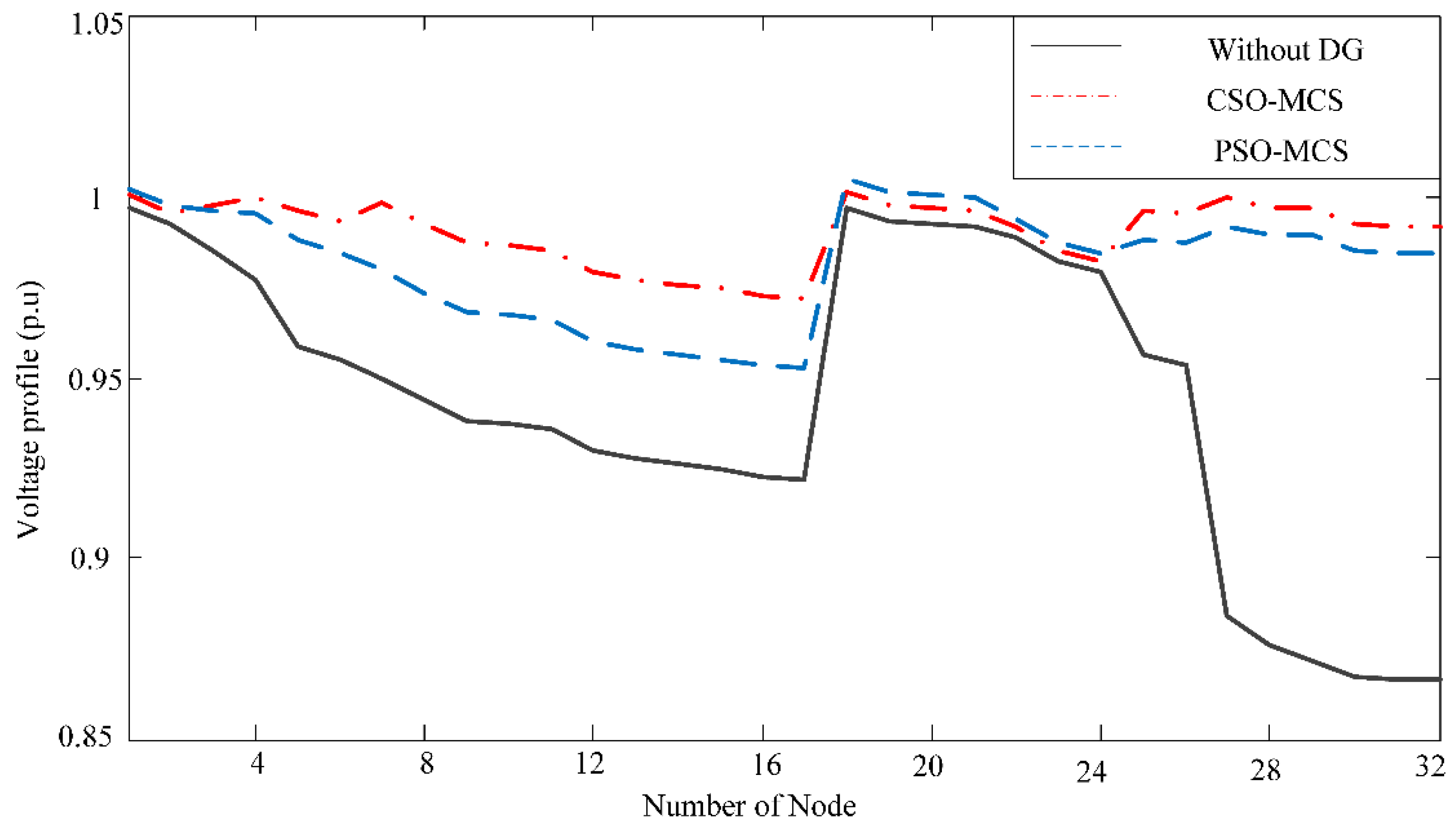
Figure 4 compares the voltage profiles of the 33-buses system before and after DG installation. The voltage profile is one of the main criterions for power quality improvement. As seen in Figure 4, the voltage quality of the origin system is dissatisfactory. The voltage of many nodes, especially the end nodes like node-31 and node-32, is seriously below the permitted range. After installing DGs according to the optimal schemes, the voltage profile is obviously improved. It can be observed that both of the methods (i.e., CSO-MCS and PSO-MCS) provide better voltage profile in the simulation. According to the statistical results, the average voltage deviation (AVD) of the scheme obtained by CSO-MCS and that by PSO-MCS is 0.00615 p.u and 0.01472 p.u, which present a reduction of 89.15% and 74.02% compare to the origin system. Meanwhile, we can see that the voltage profile obtained by CSO-MCS method is better than that by PSO-MCS in terms of average voltage deviation and voltage stability.

Figure 4. Voltage profile contrast (Case 1).

Figure 4. Voltage profile contrast (Case 1).

From the above analyses, we can draw a conclusion that CSO-MCS has good performance in terms of convergence accuracy and robustness, and it is suitable for solving DG allocation problems.

From the above simulation results, we can also evaluate the benefits brought about by optimal DG allocation. Before placing DGs in the distribution system, the emission of air pollutants is 1.3582 × 10⁵ tons. After allocating DGs using CSO-MCS algorithm, a maximal reduction of 0.298 × 10⁵ tons or approximately 21.96% of pollutant emissions can be achieved, as shown in Table 4. The significant reduction in pollutant emission reveals the great contribution of DGs to environmental protection. In terms of power losses, after placing DGs, the system loss costs reduce from 7.8783 × 10⁵ $ to 5.1482 × 10⁵ $, which proves that reasonable application of DGs can effectively reduce the system network losses.

5.2. Case 2: PG&E 69-Bus System

A larger test system proposed in [31] is considered in this case. The base power of this system is 10 MVA and the base voltage is 12.66 kV.

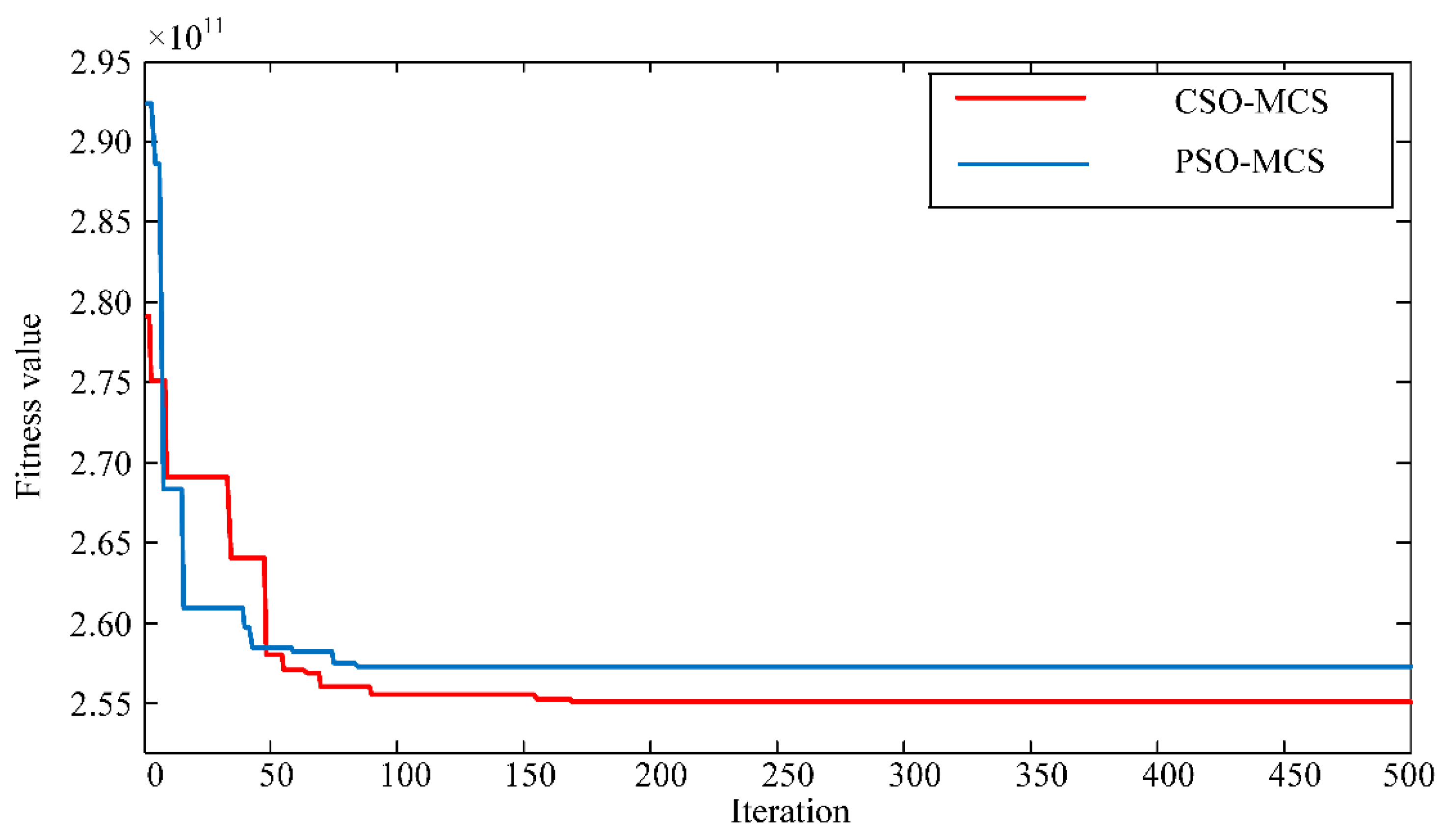
Figure 5 shows the convergence characteristics obtained by CSO-MCS and PSO-MCS. As shown in this figure, it is obvious that CSO-MCS outperforms PSO-MCS in terms of searching for better converged solutions. The optimal fitness value of CSO-MCS is 0.704% better than that of PSO-MCS.

The simulation results obtained by CSO-MCS are shown in Table 5 and compared with the results of PSO-MCS. According to the results reported in Table 5, it can be observed that CSO-MCS is capable of finding better solutions. The minimum of pollutant emission applying CSO-MCS is 1.0772 × 10⁵ t, which is 0.706% less than the best results of PSO-MCS. Similar results can be found in the power losses cost index. As seen in Table 5, the power losses cost achieved by CSO-MCS is 22.39% less than that by PSO-MCS.

Figure 5. Convergence characteristics of CSO-MCS and PSO-MCS (Case 2).

Figure 5. Convergence characteristics of CSO-MCS and PSO-MCS (Case 2).

Table 5. Results obtained by CSO-MCS and PSO-MCS (30 runs for Case 2).

Evaluation method		Pollutant emissions (105 t)	Power losses cost (105$)	Total DG cost (106$)	CPU time (s)
CSO-MCS	Maximum value	1.0859	5.8827	5.1555	589.92
	Minimum value	1.0772	5.4875	5.0689	572.24
	Mean	1.0820	5.7526	5.1121	583.92
	Standard deviation	0.0027	0.0778	0.0272	5.16
PSO-MCS	Maximum value	1.1168	7.2021	4.2893	639.38
	Minimum value	1.0848	6.7160	4.0818	595.26
	Mean	1.1002	7.0458	4.1956	615.80
	Standard deviation	0.0097	0.1041	0.0637	14.29

Table 5. Results obtained by CSO-MCS and PSO-MCS (30 runs for Case 2).

Evaluation method		Pollutant emissions (105 t)	Power losses cost (105$)	Total DG cost (106$)	CPU time (s)
CSO-MCS	Maximum value	1.0859	5.8827	5.1555	589.92
	Minimum value	1.0772	5.4875	5.0689	572.24
	Mean	1.0820	5.7526	5.1121	583.92
	Standard deviation	0.0027	0.0778	0.0272	5.16
PSO-MCS	Maximum value	1.1168	7.2021	4.2893	639.38
	Minimum value	1.0848	6.7160	4.0818	595.26
	Mean	1.1002	7.0458	4.1956	615.80
	Standard deviation	0.0097	0.1041	0.0637	14.29

With respect to computing speed, the mean CPU time of CSO-MCS is 583.92 s, which is 5.46% less than that of PSO-MCS. Besides, it is worthwhile to note that CSO-MCS also shows good performance on robustness. It can be observed from Table 5 that the standard deviation of emissions index achieved by CSO-MCS is 0.0027 × 10⁵ t, whereas the standard deviation value obtained by PSO-MCS is 0.0097 × 10⁵ t. In terms of other indices, the power losses cost index, total DG cost index and CPU time index achieved by the proposed algorithm are smaller than those achieved by PSO-MCS. The above analysis results of 69-bus test system further confirm the effectiveness and robustness of CSO-MCS in solving DG allocation problems.

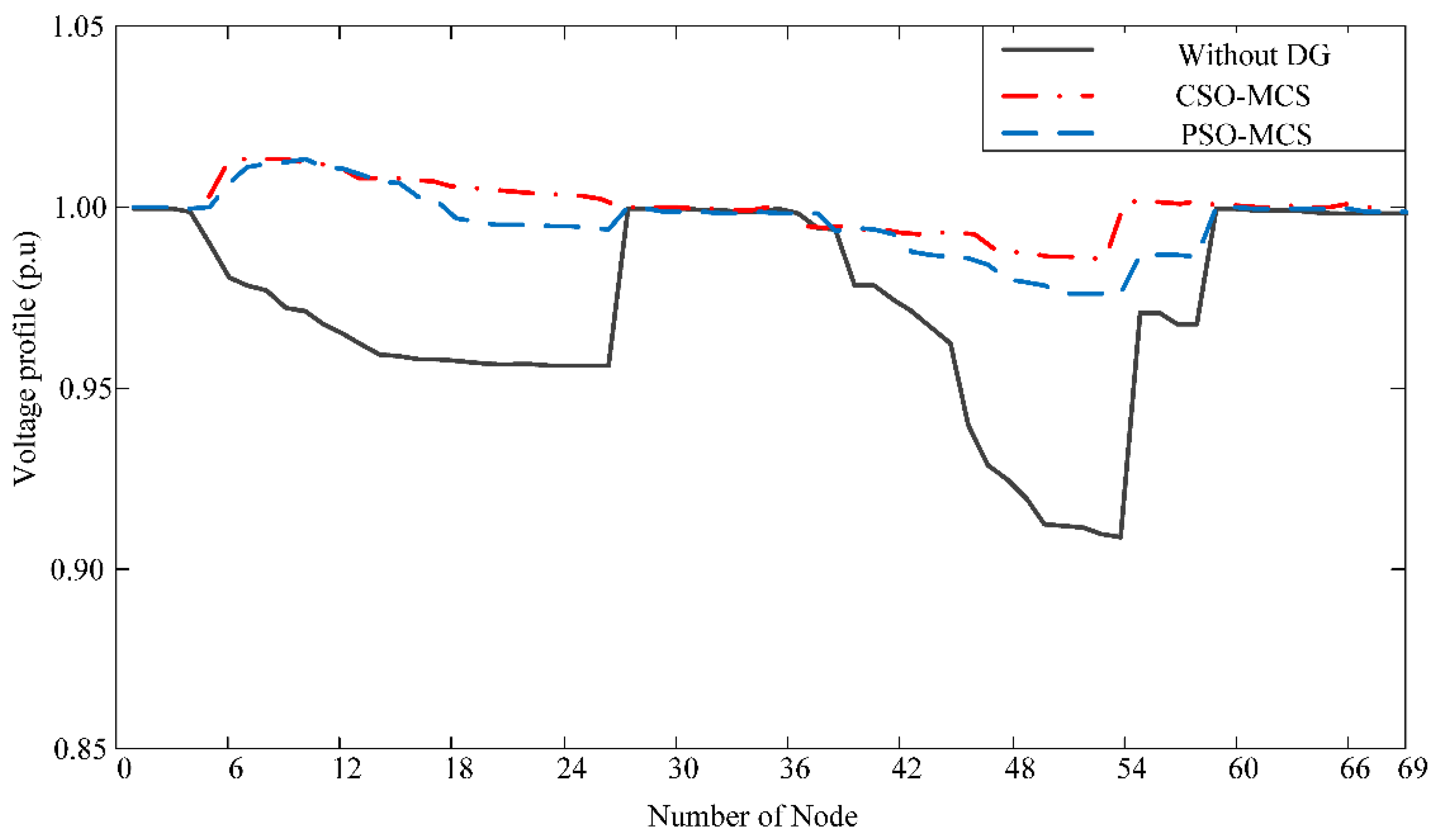
Figure 6 shows and compares the mean voltage magnitude of each node for the 69-bus system using different methods. From this figure, it can be observed that the voltage amplitude of many nodes of the origin system is seriously below the permitted range. After placing DGs using the optimization methods, we can see that a marked improvement in voltage profiles can be achieved. As seen in Figure 6, before placing DGs, the original voltage magnitude of node 54 is 0.909 p.u. After optimizing DG allocation in the distribution system, the voltage magnitude of node 54 increases to 0.986 p.u. Similar results have been seen in other nodes. In addition, according to the statistical results, the average voltage deviation (AVD) obtained by CSO-MCS is 0.005 p.u, which has a reduction of 81.62% compare to the origin system. When comparing the voltage profiles obtained by the two algorithms (i.e., CSO-MCS and PSO-MCS), we can see that the AVD achieved by CSO-MCS is also less than the results that of PSO-MCS (0.007 p.u), which also indicates the validity of CSO-MCS in solving ODGA problem.

Figure 6. Voltage profile contrast (Case 2).

Figure 6. Voltage profile contrast (Case 2).

5.3. Influence of Uncertainties of Renewable DGs

In order to investigate the effect of uncertainties of renewable energy on the planning results, two scenarios have been designed in Table 6. The stochastic characteristics of renewable energy can be described by their probability density functions (PDF). In this simulation, we design two sets of PDF parameters of renewable energy (i.e., shape and scale parameters of the Weibull distribution of wind speed; shape parameters of the Beta distribution of solar radiation). Scenario B shows higher level of wind speed and lower level of solar illumination in comparison to Scenario A. The results associated with the schemes for the 33-bus and 69-bus systems are shown in Table 7 and Table 8. With respect to the chance constraints of voltage amplitude and power flow, statistical results indicate that, for the 33-bus system, the probabilities of voltage chance constraint Pr{V_min ≤ V ≤ V_max} are 0.954 and 0.962; for the 69-bus system, the probabilities of voltage chance constraint Pr{V_min ≤ V ≤ V_max} are 0.937 and 0.942. In terms of the chance constraint of power flow, the probabilities Pr{S_ij ≤ S_max} are 0.922 and 0.937 for the 33-bus system; 0.920 and 0.929 for the 69-bus system. Both of the probabilities can satisfy the given value (i.e., α = β = 0.9), so the optimization results are acceptable. Besides, from Table 7, we can observe that the obtained results vary with the uncertain characteristics of renewable energy. The penetration of WT-based DG is increased from 300 kW (Scenario A) to 500 kW (Scenario B), whereas the installation of PV-based DG is decreased from 610 kW (Scenario A) to 370 kW (Scenario B). Similar change of optimization results appeared in the 69-bus system. The main reason for this change is due to the higher level of wind speed and the lower level of solar illumination intensity in Scenario B. Using the stochastic feeder loads, wind power outputs, photovoltaic power outputs and other data in Table 1, Table 2 and Table 3, the voltage distributions under different scenarios can be evaluated by using the proposed method. To investigate the variation of voltage profile of the distributed system caused by embedded renewable DGs, we select two representative nodes from the two test systems respectively, and draw their voltage probability density curves in Figure 7, Figure 8, Figure 9 and Figure 10. In the 33-bus system, one of the representative nodes is the 4th node, which has large sizes of DGs. Another is the 32nd node, which has no DGs and locates at the end of the system. In the 69-bus system, the representative node with large capacity of DGs is the 14th node, and the other node without DGs is the 50th node.

Table 6. Definition of two scenarios.

Scenario	Wind speed parameters	Solar radiation parameters
A	k = 1.80, c = 6	α = 2.0, β = 2.0
B	k = 2.15, c = 9	α = 0.9, β = 0.9

Table 6. Definition of two scenarios.

Scenario	Wind speed parameters	Solar radiation parameters
A	k = 1.80, c = 6	α = 2.0, β = 2.0
B	k = 2.15, c = 9	α = 0.9, β = 0.9

Table 7. Optimization results of different scenarios (33-bus system).

DG type	Candidate location	DG sizes (kW)
		Scenario A	Scenario B
WT	4	120	200
	18	180	300
	25	0	0
	32	0	0
PV	4	220	120
	7	200	150
	25	100	40
	29	90	60
MT	4	120	40
	7	80	120
	17	150	50
	29	0	40

Table 7. Optimization results of different scenarios (33-bus system).

DG type	Candidate location	DG sizes (kW)
		Scenario A	Scenario B
WT	4	120	200
	18	180	300
	25	0	0
	32	0	0
PV	4	220	120
	7	200	150
	25	100	40
	29	90	60
MT	4	120	40
	7	80	120
	17	150	50
	29	0	40

Table 8. Optimization results of different scenarios (69-bus system).

DG type	Candidate location	DG sizes (kW)
		Scenario A	Scenario B
WT	14	150	100
	20	30	0
	26	0	20
	46	80	20
	49	60	30
	52	120	80
	53	200	120
PV	14	100	200
	20	0	40
	26	0	0
	46	20	50
	49	50	90
	52	100	170
	53	100	150
MT	14	150	90
	20	0	20
	26	10	0
	46	0	0
	49	60	80
	52	150	100
	53	100	80

Table 8. Optimization results of different scenarios (69-bus system).

DG type	Candidate location	DG sizes (kW)
		Scenario A	Scenario B
WT	14	150	100
	20	30	0
	26	0	20
	46	80	20
	49	60	30
	52	120	80
	53	200	120
PV	14	100	200
	20	0	40
	26	0	0
	46	20	50
	49	50	90
	52	100	170
	53	100	150
MT	14	150	90
	20	0	20
	26	10	0
	46	0	0
	49	60	80
	52	150	100
	53	100	80

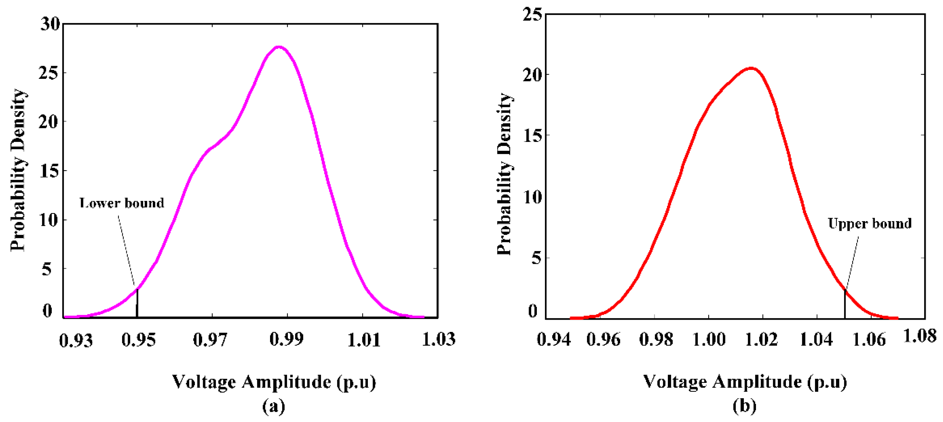
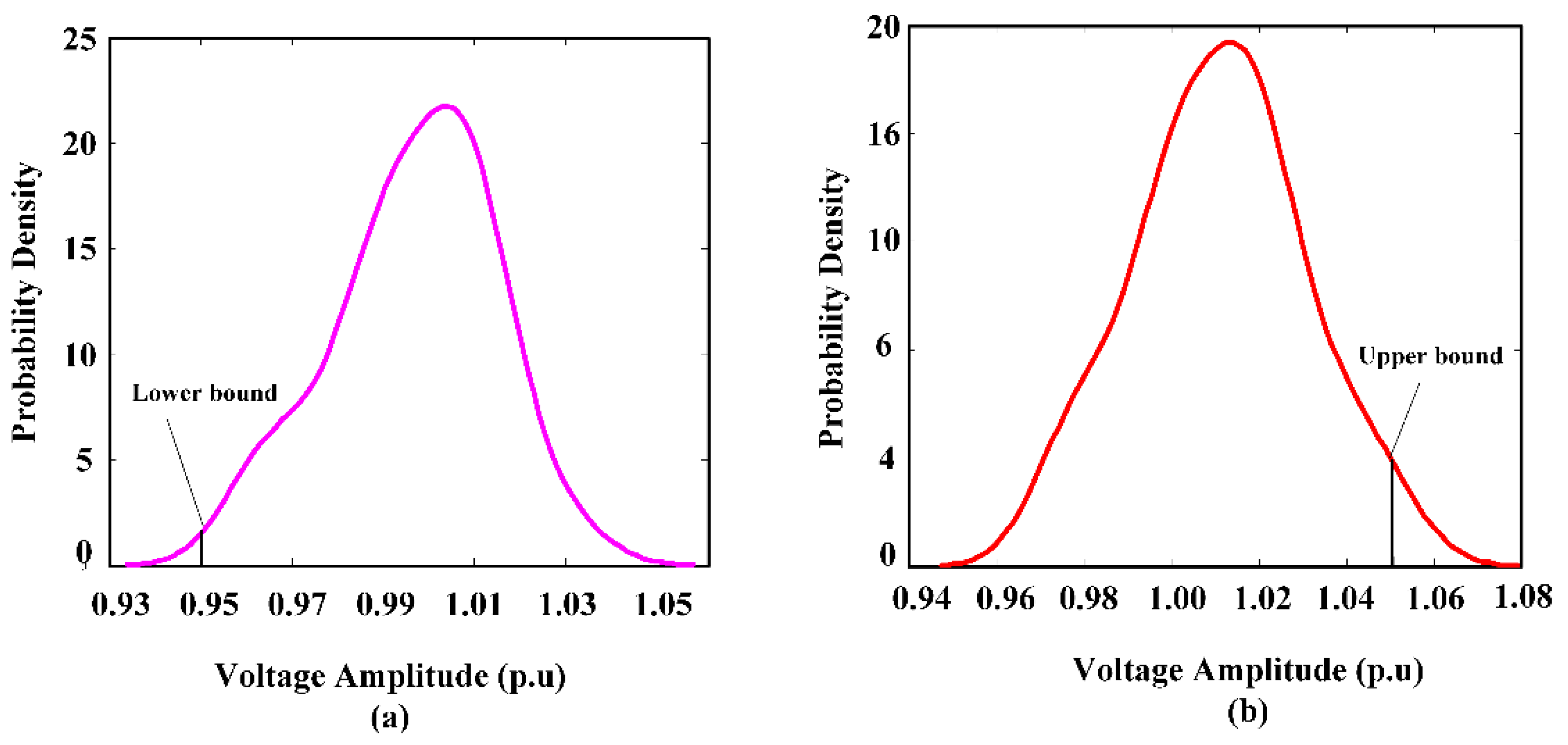
Figure 7. PDF curve of voltage amplitude in Scenario A of 33-bus system: (a) Node 32 and (b) Node 4.

Figure 7. PDF curve of voltage amplitude in Scenario A of 33-bus system: (a) Node 32 and (b) Node 4.

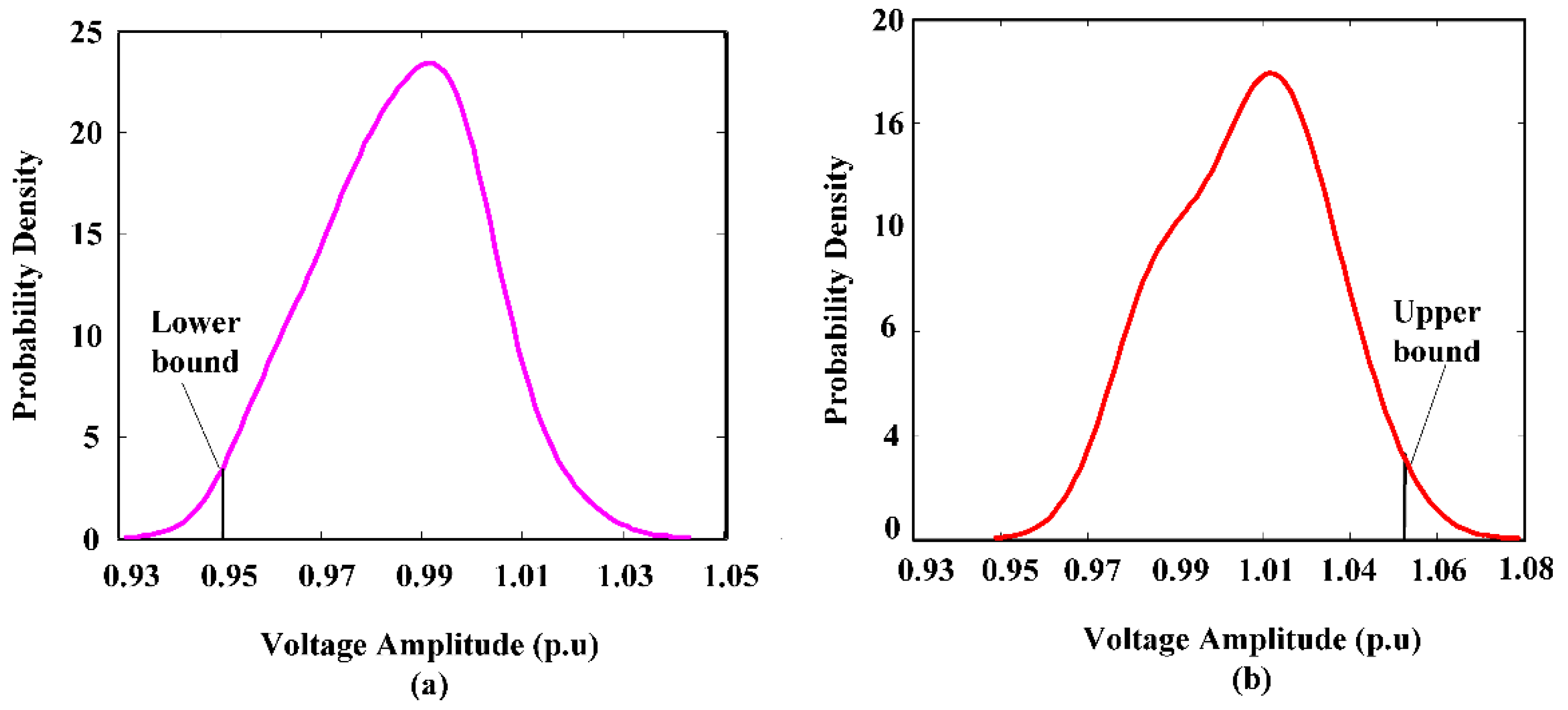
Figure 8. PDF curve of voltage amplitude in Scenario B of 33-bus system: (a) Node 32; (b) Node 4.

Figure 8. PDF curve of voltage amplitude in Scenario B of 33-bus system: (a) Node 32; (b) Node 4.

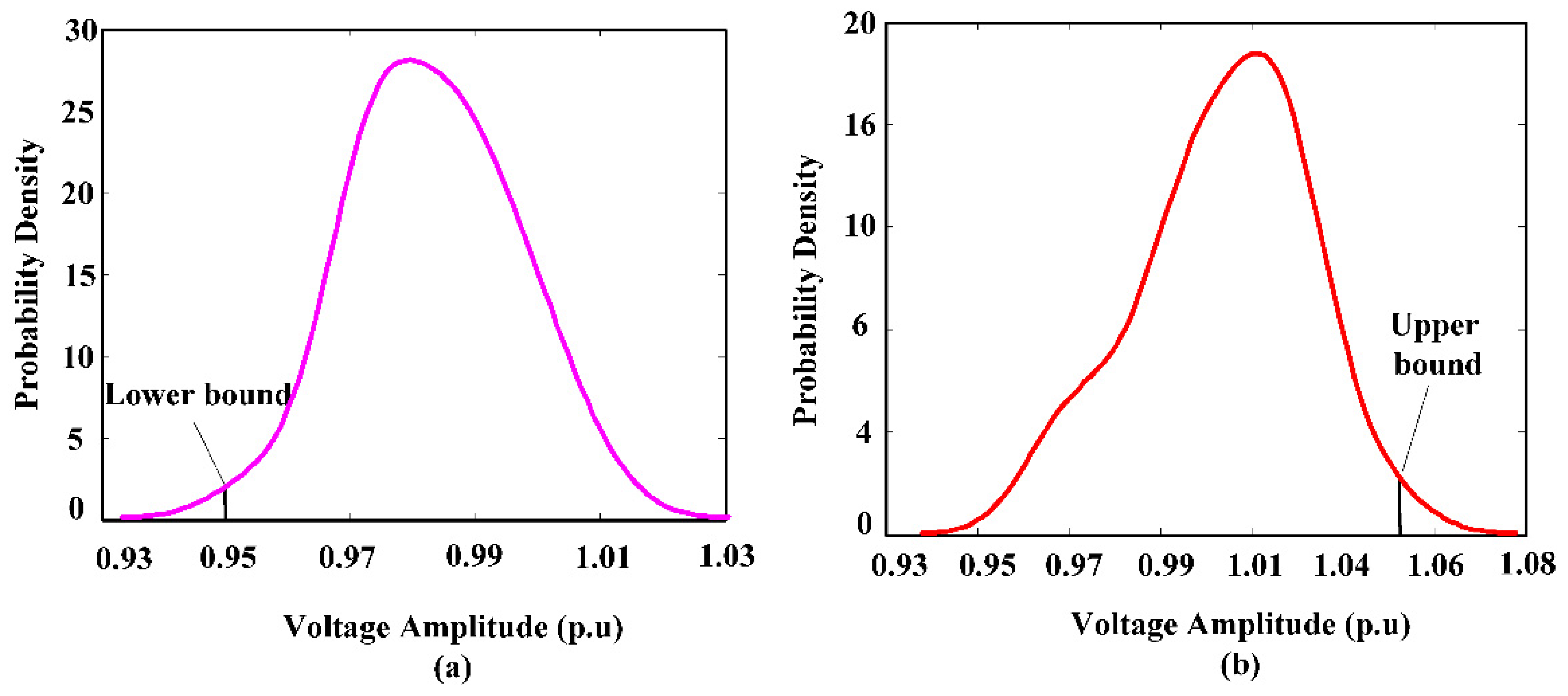
The voltage probability density curves of node 4 and node 32 indicate that the voltage profile is obviously improved after placing DGs properly. From Figure 7 to Figure 10, we can see that in most cases of the 33-bus system, the voltage of node 32 distributes between 0.98 p.u and 1.00 p.u, and the voltage of node 4 distributes between 0.99 p.u and 1.03 p.u. As for the 69-bus system, we can observe that the voltage of node 50 distributes between 0.985 p.u and 0.995 p.u, and the voltage of node 14 distributes between 0.98 p.u and 1.02 p.u. Both of them are within the allowable range for power systems to ensure the operation safety. However, it is worthwhile to note that the voltage amplitudes of the two nodes may sometimes exceed the limitation, due to the intermittent of DG power supply. Thus, for those important customers whom are sensitive to voltage quality and locate close to DG connected nodes, it is necessary to make measures to keep stable voltage quality.

Figure 9. PDF curve of voltage amplitude in Scenario A of 69-bus system: (a) Node 50 and (b) Node 14.

Figure 9. PDF curve of voltage amplitude in Scenario A of 69-bus system: (a) Node 50 and (b) Node 14.

Figure 10. PDF curve of voltage amplitude in Scenario B of 69-bus system: (a) Node 50 and (b) Node 14.

Figure 10. PDF curve of voltage amplitude in Scenario B of 69-bus system: (a) Node 50 and (b) Node 14.

6. Conclusions

Integration of distributed generations into the distribution system may change various operating characteristics of the system, especially at increased penetration of renewable DGs like wind power and photovoltaic generation. This paper has proposed a novel approach integrating crisscross optimization algorithm and Monte Carlo simulation called CSO-MCS is proposed to effectively obtain the best sizes, locations and types of DGs in the distribution system. The proposed CSO-MCS method is compared with PSO-MCS in terms of convergence and computation time to demonstrate its effectiveness and feasibility. Furthermore, an optimization framework for optimal DG allocation problem using chance constrained programming (CCP) is presented in this paper. The objective functions encompass minimization of total pollutant emission, DG cost and active power losses over the planning period. In order to assure the feasibility of planning results, the system uncertainties covering wind speed, solar radiation and load consumption are taken into account using their probabilistic models.

This proposed work can help the system operators in evaluating DG allocation schemes to decide the best feasible solution for practical implementation and enable them to evaluate the impact of system uncertainties on DG planning work. As future work, we are preparing to apply CSO-MCS to address more practical ODGA problems considering reliability impacts and other factors, then conduct a research on the system operation and energy management of a smart distribution grid connecting large numbers of DGs and PEVs.