Article

Predicting Iron Losses in Laminated Steel with Given Non-Sinusoidal Waveforms of Flux Density

1
College of Electrical Engineering, Zhejiang University, Hangzhou 310058, China
2
China Academy of West Region Development, Zhejiang University, Hangzhou 310058, China
*
Author to whom correspondence should be addressed.
Energies 2015, 8(12), 13726-13740; https://doi.org/10.3390/en81212384
Submission received: 8 September 2015 / Revised: 8 November 2015 / Accepted: 18 November 2015 / Published: 3 December 2015

Abstract

:
In electrical machines, iron losses are essential for electromagnetic and thermal designs and analyses. Although many models have been proposed to predict iron losses in magnetic materials, the calculation of iron losses under non-sinusoidal excitations is still an open field. Most works concern the influences of the value, the change rate or the frequency of flux density in the frequency domain. In this paper, we propose an engineering model for predicting loss characteristics with given waveforms of flux density in the time domain. The characteristics are collected from the knowledge of the iron loss in a laminated ring-shaped transformer. In the proposed model, we derive mathematical formulas for exciting currents in terms of flux density by describing the function methods through multi-frequency tests with sinusoidal excitations. The non-linearity of the material is interpreted by branches of conductances accounting for hysteresis and eddy-current losses. Then, iron losses are calculated based on the law of conservation of energy. An experimental system was built to evaluate the magnetic properties and iron losses under sinusoidal and non-sinusoidal excitations. Actual measurement results verify the effectiveness of the proposed model.

1. Introduction

Recently, various types of excitation conditions were applied to electrical machines with power electronics technology. The use of pulse width modulation (PWM) and non-linear loads results in a difficulty in iron loss prediction in magnetic materials. Although many models, which are based on physical or numerical methods [1,2,3,4,5,6,7,8,9], have been proposed by different researchers, predicting iron losses in magnetic materials, when a non-sinusoidal voltage excitation is applied, has not yet been entirely solved and is still an open research field.
Following the modern research on iron losses in magnetic materials, iron losses can be decomposed into three main components, referred to as hysteresis, eddy-current and excess losses. (1) Hysteresis losses are due to the steady losses of the Weiss domains and are supposed to depend on excitations and be independent of the structures and lamination thickness of iron cores; (2) on the contrary, eddy-current losses are due to the existence of eddy-currents and are affected by structures and lamination thickness, which affect the distribution and intensity of the eddy-current; (3) excess losses are due to dynamic losses of the Weiss domains caused by block walls’ discontinuous movements with the production of the Barkhausen jumps [10,11]. Based on the above contents, the Steinmetz equation [1] was proposed a century ago and has been widely used for iron loss estimation under sinusoidal excitations. With various structural arrangements and magnetization inputs applied to electrical machines, estimations of iron losses based on the steel manufacturers’ datasheets, which mostly are tested under sinusoidal excitations, will exhibit large deviations from the actual ones. Over the last few decades, models have been established to improve the accuracy of the Steinmetz equation for various excitations, such as MSE (modified Steinmetz equation) [4,12,13,14], GSE (general Steinmetz equation) [15,16] and iGSE (improved general Steinmetz equation) [17]. MSE uses the change rate of excitations instead of frequency. GSE suggests that iron losses are related to the transient and historical values of flux density. iGSE combines the idea of the MSE and GSE methods. Some variability and correlation of the loss coefficients are introduced, including a form factor [5,6] and equivalent frequency [12,13] coefficients for PWM excitations and a three-order polynomial representation of the hysteresis-loss multiplicative coefficient [4,14,18]. Research papers pointed out that iron loss prediction should depend on frequency, magnitude, change rate and historical values of flux density, as well as other factors. Thus, the most accurate result would require a time-domain simulation on the typology of actual waveforms and the non-linearity of magnetic properties, which includes all loss information of flux density B and magnetic field H.
Compared to hysteresis losses and eddy-current losses, excess losses are usually small enough to be neglected under low and medium frequency operations in laminated steel [7,19]. Once the structure and material model of the iron core are determined, iron losses can be assumed to be only related to the alternating magnetic fields, which can be described as waveforms of flux density. The flux density is a vector with an alternating magnitude and direction. For the work at hand, only the alternating magnitude of the flux density is considered for the iron loss calculation under the steady state. The most frequently-used materials for electrical machines are non-oriented silicon steel, in which losses with the same magnitude, but different directions can be assumed to be the same according to its isotropy. In this way, iron losses can be predicted by analyzing the relationship between flux density and iron losses in the time domain.
Based on the above contents, we established an engineering model for predicting iron losses under non-sinusoidal excitations by using multi-frequency sinusoidal data together with given waveforms of flux density. The rest of this paper is organized as follows. Section 2 presents the experimental system containing a wound ring core with a small air gap for magnetic property and iron loss evaluation. Section 3 introduces the calculation procedure of the proposed engineering model. Section 4 compares the proposed model with actual measurement results under two types of excitations. Conclusions are presented in Section 5.

2. Specimen and Measurement System

The most common industrial measurement system for magnetic property measurement of silicon steel is based on the Epstein frame, which has the advantage of the possibility of material replacement. Although its accuracy is sufficient for industrial applications, the flux density distribution in the joints of the iron core is non-uniform and deviates from its main direction. Ring frames are often used for academic research under alternating excitation [20], which has the advantages of uniform magnetic field distribution and a simple magnetic path. Figure 1 shows the setup of a specimen and the schematic diagram of the experimental system, which consists mainly of an iron core, a programmable AC + DC power supply and a Gauss meter for flux density measurement under DC conditions and low frequency excitations. Stranded wires were wound uniformly around the laminated iron core, forming the exciting coil. One unit of the stranded wires was separated to form the B-coil. In this way, the influence of leakage flux is minimized, and the measurement of input and induced voltage achieves a good coupling effect with the same distribution and shared ground point. Table 1 shows the parameters of the ring frame with a small air gap. The specimen model is 50WW470 (non-oriented, density: 7.7 kg/dm 3 ; lamination thickness: 0.5 mm; iron loss: 3.25 W/kg at 1.5 T and 50 Hz).
The iron core was excited by the programmable voltage supply with a controlled frequency, amplitude and harmonic ratio. Input currents were obtained by current viewing resistance R z (0.01 Ω) through a coaxial cable, which minimizes the time difference between current and voltage waveforms. The resistances of R d , R z and the exciting coil were measured with a Kelvin bridge (QJ84A) with temperature rises taken into consideration. It was found that R z barely changes with temperature rises. Two methods were used to measure the flux density B in the iron core. In the conditions of DC and low frequency (up to 400 Hz) excitations, the flux density was acquired by the Gauss meter (Lakeshore 460) with a plate probe (MNT-4E04-VH), which is sealed by wax inside the air gap. Under AC conditions, the flux density was calculated as:
B = u 2 ( t ) d t N 2 S
where:
u 2 ( t )
 induced voltage of the B-coil;
N 2
     turn number of the B-coil;
S 
   section area of the magnetic core.
Figure 1. Setup of the specimen and experimental system. (a) Arrangement of the specimen; (b) Schematic diagram of the experimental system.
Energies 08 12384 g001
Table 1. Parameters of the specimen.
ItemParameter
Model50WW470
Inner diameter230 mm
Outer diameter250 mm
Thickness10 mm (20 sheets)
Air gap2 mm
Turn number of exciting coil1000 turns
Turn number of B-coil1000 turns
Magnetic path length751.55 mm
Resistance of exciting coil0.3615 Ω
Cross-sectional area of exciting coil6.627 mm 2

3. Engineering Model for the Iron Loss Calculation

3.1. Sinusoidal Excitations

The ring frame can be expressed as two circuit models, shown in Figure 2 [21]. In the linear model, R copper is the resistance of the exciting coil, L s is the leakage inductance, R e is the resistance accounting for eddy-current losses and L m is the inductance of the exciting coil. Experimental results indicated that winding resistances and leakage inductances could be considered to be constant for the tested transformer; hence, it was assumed that all non-linearity could be confined to the core. In the non-linear model, G h i and G e are the conductances accounting for hysteresis and eddy-current losses, respectively. The small boxes in series with G h i are ideal filters, which allow only specific harmonic components of the current i h to flow to corresponding G h . In this paper, the resistance and inductance of wires that connect the exciting coil and the power supply are ignored. According to the law of conservation of energy, the iron loss in the iron core under no-load conditions can be calculated as:
W = ( u 1 i i 2 R c o p p e r ) d t = N 1 N 2 u 2 i d t + L s i 2 d t
The iron loss of leakage flux was neglected with uniform windings, so the average iron loss in one cycle can be expressed as:
P = 1 T 0 T N 1 N 2 u 2 i d t
where:
u 1 ( t )
  exciting voltage;
i 
    exciting current;
N 1
     number of turns of the exciting coil;
N 1 N 2 u 2
   induced voltage transformed to the primary side;
P 
      average iron loss in one cycle.
In this way, all we need for the iron loss calculation are the waveforms of the induced voltage and exciting current. When the waveforms of the flux density are given, the relationship between the induced voltage and flux density is described by Equation (1). Therefore, the last thing is predicting the exciting current under the given flux density for Equation (2). Figure 3 illustrates the process of the iron loss calculation, in which f ( B ) is the non-linear describing function of the exciting current in terms of the flux density. In Figure 3, the waveforms of flux density are obtained by Equation (1), and the current waveform is calculated using the describing functions. Then, the iron loss is calculated based on both voltage and current waveforms.
Figure 2. Equivalent circuits for the experimental specimen. (a) Linear transformer model; (b) Nonlinear model.
Energies 08 12384 g002
Figure 3. Process of the iron loss calculation.
Energies 08 12384 g003
When related to a sinusoidal induced voltage, the magnetic flux density can be expressed by:
u 2 ( t ) = U m sin ( ω t ) = N 2 S d B d t
B ( t ) = U m N 2 S ω cos ( ω t ) = B m cos ( ω t )
where:
U m
   amplitude of the induced voltage;
ω 
    angular frequency;
B m
   amplitude of the flux density.
In a steady state, the exciting current is a periodic function and can be obtained through non-linear components of the core conductances, as shown in Figure 4. Figure 4 illustrates the relationship between the flux density and exciting current, where B ( t ) is the flux density, i ( t ) is the non-sinusoidal exciting current and the relationship is defined as a hysteresis loop. Exciting current i ( t ) is expressed mathematically by three-order polynomials, with a goodness of fit r 2 greater than 0.95, in terms of the flux density piecewise. The lower curve of the hysteresis loop is divided into three segments by knee points ( M 1 , i k 1 ) and ( M 2 , i k 2 ), according to the saturation and non-saturation sections. When no DC-bias is involved, the hysteresis loop is an odd function. Thus, i ( t ) is written as:
i ( t ) = f ( B ( t ) ) = a 0 + a 1 B ( t ) + a 2 B 2 ( t ) + a 3 B 3 ( t ) 0 ω t < β 1 a 4 + a 5 B ( t ) + a 6 B 2 ( t ) + a 7 B 3 ( t ) β 1 ω t < β 2 a 8 + a 9 B ( t ) + a 10 B 2 ( t ) + a 11 B 3 ( t ) β 2 ω t < π
where:
a i
   parameters of the three-order polynomials;
β i
   corresponding phase angle of the knee points.
Figure 4. Waveforms of the exciting current with corresponding flux density.
Energies 08 12384 g004
Application of a fast Fourier transform (FFT) algorithm is then used to convert the exciting current to the frequency domain.
i ( t ) = A 0 2 + k = 1 A k cos ( k ω t ) + k = 1 B k sin ( k ω t ) I k = A k 2 + B k 2 φ k = arctan ( A k B k )
The iron loss can be calculated by:
P M = 1 M T 0 T N 1 N 2 u 2 i d t = 1 2 M N 1 N 2 k = 1 U k I k cos ( Δ φ k )
where:
A k , B k
   harmonic magnitude;
I k
         harmonic amplitude of the exciting current;
φ k
        harmonic phase angle of the exciting current;
U k
        harmonic amplitude of the induced voltage;
Δ φ k
  harmonic phase angle difference between the induced voltage and exciting current;
M 
        mass of the specimen.
In this case, U 1 = U m and U k , 2 k < = 0 , the iron loss density can be expressed by:
P M = 1 2 M N 1 N 2 U m I 1 cos ( Δ φ 1 )

3.2. Non-Sinusoidal Excitations

When a periodic, non-sinusoidal voltage is applied without the considerations of DC-bias and minor loops, the induced voltage can be converted into a sum of sine-functions as in Equation (10). Meanwhile, the flux density can be expressed by Equation (11).
u 2 ( t ) = n = 1 U m p n sin ( n ω t + φ u , n )
B ( t ) = n = 1 B m p n n cos ( n ω t + φ u , n ) = n = 1 B n ( t )
where:
p n
         harmonic content of the induced voltage;
φ u , n
       harmonic phase angle of the induced voltage;
B n ( t )
     harmonic component of the flux density.
When the waveforms of the flux density are known, harmonic amplitude and phase angles of the induced voltage and flux density can be easily obtained. A series of describing functions f n ( B n ( t ) ) for the n-th order of harmonics of B-I loops with the same B peak value as the given waveforms of flux density is pre-calculated according to Section 3.1. The parameters of the describing functions, which are used in the following sections, are listed in the Appendix. The function of the n-th harmonic of the exciting current is described as i n = f n ( B n ( t ) ) = F ( n , ω , β 1 , n , β 2 , n , B peak ) . It is known that each order of harmonics is not mutually independent of the others, and the total exciting current is different from the superposition of i n . Making reference to the influence of one harmonic of the exciting current on the flux density, the same change of the current results in different changes of the flux density depending on the saturation level of the iron core. Indeed, the influence of each order of harmonics depends on both magnitudes and corresponding transient variations. The exciting current and iron loss under non-sinusoidal excitations can be calculated mathematically as follows:
Step (1)  
Obtain describing functions in the same form as Equation (6) with various frequencies and B peak values by multi-frequency tests under sinusoidal excitations.
Step (2)  
Convert the non-sinusoidal waveforms of flux density into a series of sinusoidal waves and sample all waves with an interval time Δ t .
Step (3)  
Initialize fundamental and harmonics of the exciting current as follows:
i n ( 0 ) = I 0 , n
where I 0 , n is a random value and 1 n < .
Step (4)  
Define ( ω t ) as follows,
( ω t ) = n ω t + φ u , n
The position of B n ( t ) in the corresponding I ( B ) curve as shown in Figure 4 is found using the value of ( ω t ) . The corresponding describing function f n ( B n ( t ) ) is applied to calculate the change of the n-th harmonic of the exciting current by:
Δ i n ( t ) = i n ( t + Δ t ) i n ( t ) = f n ( B n ( t + Δ t ) ) f n ( B n ( t ) )
Step (5)  
Calculate the average value of the n-th harmonic of the exciting current, I a v g , n . As no DC-bias is involved in the waveforms of flux density, the average value should be equal to zero, which suggests that:
i n ( 0 ) = I 0 , n I a v g , n
i n ( t ) = i n ( t ) I a v g , n
Step (6)  
Apply FFT on the sum of the harmonics of the exciting current to obtain amplitude and phase angles, which are substituted into Equation (8) to calculate the iron loss.
The iron losses in this laminated steel under given non-sinusoidal waveforms of flux density can be calculated using this model by following Steps 1–6; the same process can be applied for iron loss calculation in other materials. Thus, the relationship between iron losses and waveforms of flux density is found using this model. It should be mentioned that the loss is calculated in units of W/kg. The iron loss calculation in electrical products, such as electrical machines, can be carried out with supplementary magnetic field simulation results. Once the FEM simulation is carried out, for each element, the weight and flux density can be derived, and the iron loss for each element could be calculated accordingly. The iron loss in the electrical machine can be obtained simply as the sum of the loss in each element.

4. Verification of the Engineering Model

For most electrical machine applications, the contents of harmonics over 10th order are likely to be tiny, and even orders are usually eliminated due to the structural arrangement. During the simulations and experiments, odd orders from first to 13th were taken into consideration for the iron loss prediction. Fifty Hertz was chosen as the fundamental frequency.

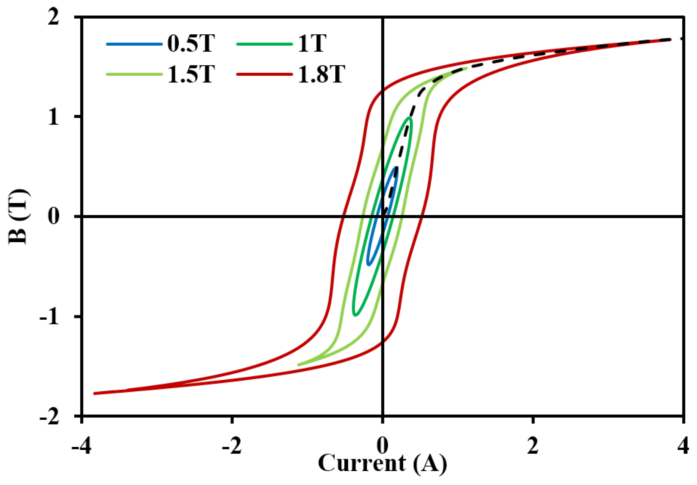
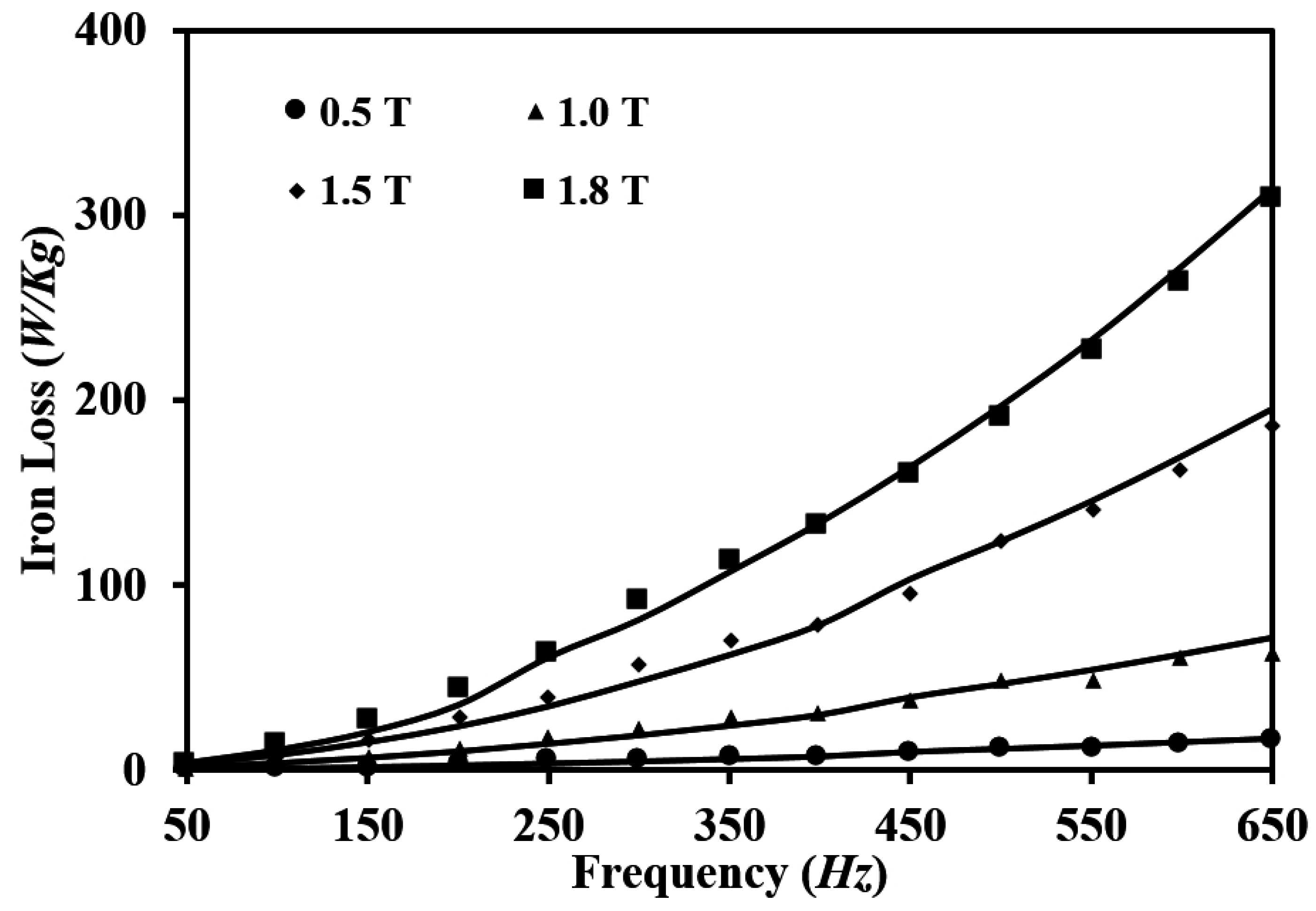
4.1. Magnetic Properties under Sinusoidal Excitations

Firstly, the experimental work of the ring frame under DC and sinusoidal excitations (from 0 to 650 Hz with a 50-Hz interval) was carried out to build the describing functions for further research, and the results were compared to those provided by the manufacturer of the Epstein apparatus. Many tests were taken to obtain B-I curves with various frequencies, and one example of 50 Hz is shown in Figure 5. Figure 6 illustrates the results of the non-linear magnetic properties and differential inductances of the ring frame with various frequencies, where the values of the horizontal axis are the logarithm (base two) of the exciting current. The inductances were calculated by:
L ( i ) = d Ψ d i = N S d B d i
where:
Ψ
 flux linkage of the exciting coil.
It can be seen that B-H curves are not in complete accord with each other. The saturation conditions of different frequencies are diverse due to the different magnetic field strength of knee points, which makes non-sinusoidal conditions more complex. The inductances also change with both frequencies and saturation levels. Only at the fully-saturated stage, the inductances seem to be independent from the frequency. Therefore, it is reasonable to consider the iron loss composition as branches in the non-linear model in Figure 2b. Figure 7 presents the iron losses in the ring frame and Epstein frame under sinusoidal voltage excitations. The results of the ring frame agree reasonably well with the data from the Epstein frame. The accuracy of the experiment system was verified for further experiments.
Figure 5. B-I curves with sinusoidal excitations at 50 Hz.
Energies 08 12384 g005
Figure 6. B-H curves and inductances with various frequencies.
Energies 08 12384 g006
Figure 7. Iron losses with various frequencies (solid lines for the Epstein frame and data points for the ring frame).
Energies 08 12384 g007

4.2. Single Harmonic Injections

The power supply was programmed to inject a single odd order of harmonics of voltage with controlled content p into the fundamental waveforms, and the amplitude of the fundamental waveforms was adjusted to achieve a constant B peak value. When B peak was 1.0 T, which happened to be near the knee point for 50-Hz excitations, the examples of seventh harmonic injections were analyzed. For seventh harmonic injections, only first and seventh orders of harmonics of the exciting current were effective for the iron loss calculation according to the composition of voltage harmonics. Both theoretical and experimental results are listed in Table 2, where the amplitudes and phase angles are obtained from the simulated and measured waveforms of the exciting currents, and P fund . and P harm . are the iron loss components calculated in Equation (8). Since the B peak value is constant, the increasing content of the seventh harmonic of injection voltage leads to a decrease in the fundamental voltage and currents. Figure 8 shows an example of the waveforms of the exciting current with 35% harmonic content. It can be seen that the results of the simulation agree well with the measured ones for amplitudes, phase angles, iron losses and waveforms. The errors of harmonic losses are below 10%, except the condition of 5% injection. It can be seen that the error of the harmonic loss becomes smaller when the content is higher. This is the result that the influence of measurement errors becomes smaller when the harmonic loss increases. The errors of fundamental and total iron losses are below 5%. The engineering model was proven to be suitable for the iron loss prediction under single harmonic injections.
Table 2. Results of 7th harmonic injections into voltage (1.0 T).
Content5101520253035404550
I 1 (A)Simu.0.37950.37660.37370.37090.36810.36540.36270.36000.35740.3548
Meas.0.38320.38240.38130.38010.37810.37740.37550.37370.37210.3700
φ 1 (rad)Simu.−1.191−1.190−1.189−1.188−1.187−1.186−1.185−1.184−1.183−1.182
Meas.−1.210−1.212−1.213−1.209−1.211−1.214−1.215−1.216−1.210−1.213
P fund . (W/kg)Simu.1.5051.4871.4691.4511.4331.4171.3991.3831.3671.355
Meas.1.4531.4321.4141.4151.3901.3671.3471.3281.3351.318
Error (%)3.623.843.892.563.133.713.874.142.412.79
I 7 (A)Simu.0.00600.01180.01760.02340.02900.03460.04000.04540.05080.0560
Meas.0.00630.01220.01840.02420.02900.03350.03900.04580.05160.0540
φ 7 (rad)Simu.−0.835−0.835−0.835−0.835−0.835−0.835−0.835−0.835−0.835−0.835
Meas.−0.690−0.759−0.739−0.732−0.826−0.878−0.838−0.838−0.884−0.907
P harm . (W/kg)Simu.0.00220.00840.01870.03320.05050.07070.09650.12430.15530.1847
Meas.0.00250.00920.02080.03690.05120.06670.09420.12530.14960.1705
Error (%)12.378.429.979.931.445.932.420.753.778.36
P total (W/kg)Simu.1.5081.4951.4871.4841.4841.4881.4961.5071.5221.540
Meas.1.4551.4411.4351.4521.4411.4331.4411.4531.4841.489
Error (%)3.593.753.632.152.973.823.783.722.543.45
Simu., Meas., fund. and harm. stand for simulation, measurement, fundamental and harmonic, respectively.
Figure 8. Comparison of the simulation and measurement results of the exciting current with 7th harmonic injections ( B peak = 1.0 T, 35% content).
Energies 08 12384 g008

4.3. Square Wave Excitations
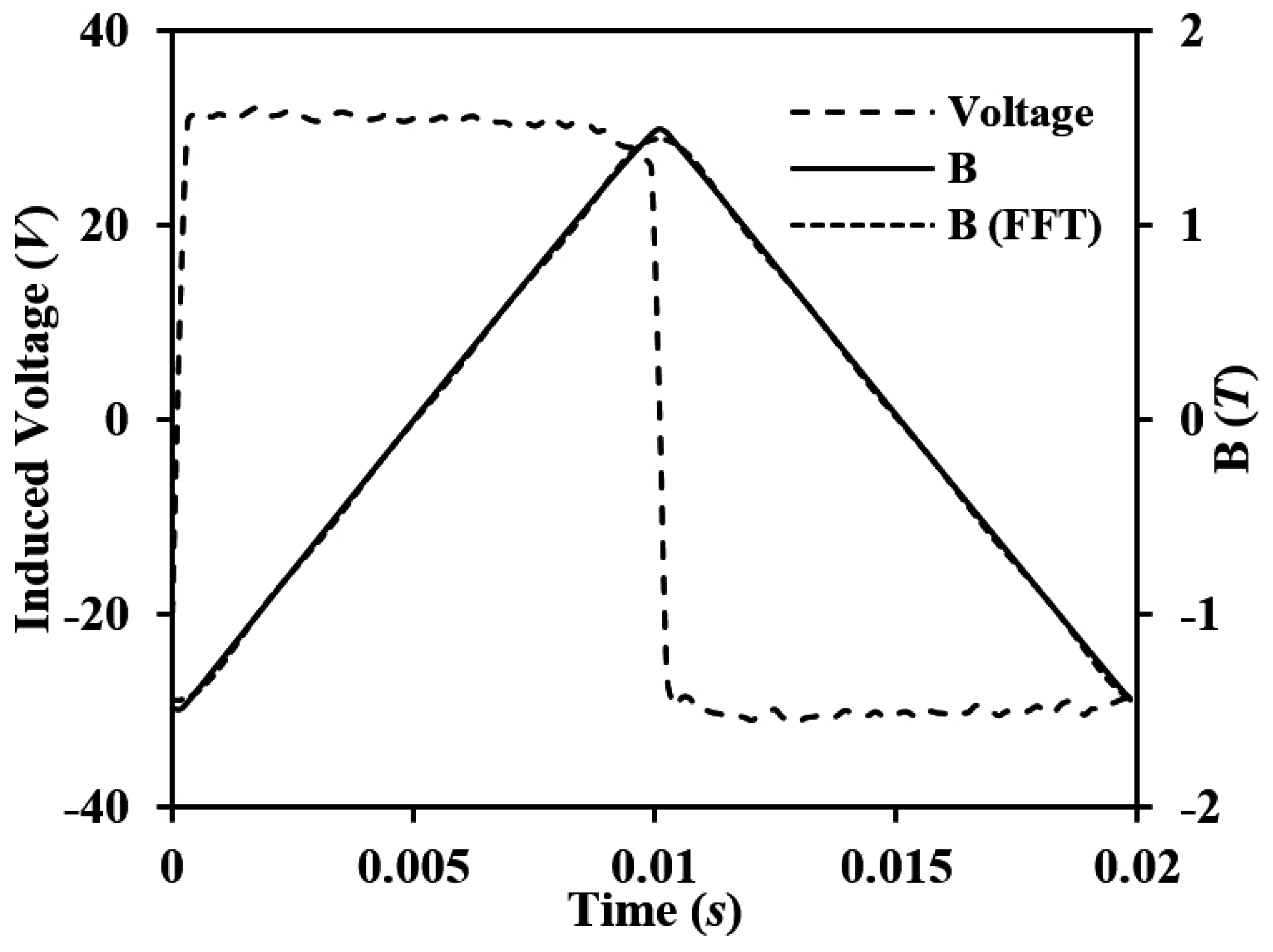
In some applications, electrical machines suffer grievous distortions. Square wave excitations are assumed to be classic among non-sinusoidal excitations. An example of 50 Hz square voltage excitations, which contains abundant harmonics, was analyzed when B peak is 1.5 T (severe saturation). Figure 9 presents the waveforms of the induced voltage and flux density, where the waveforms of voltage are square, and the flux density is triangular and can be converted into a superposition of odd orders of harmonics, as Equation (18), where orders beyond seven are ignored due to their small amplitudes.
B ( t ) = 1 . 241 cos ( ω t 0 . 015 ) 0 . 135 cos ( 3 ω t 0 . 084 ) 0 . 047 cos ( 5 ω t 0 . 149 ) 0 . 023 cos ( 7 ω t 0 . 216 )
Figure 9. Waveforms of the induced voltage, flux density and its fast Fourier transform (FFT) results under the square excitation ( B peak = 1.5 T, f = 50 Hz).
Energies 08 12384 g009
Under this condition of flux density, the iron loss was calculated according to the proposed model in Section 3.2. Table 3 shows the comparison of the simulation results with experiments, and Figure 10 illustrates the waveforms of the exciting current. The waveforms of the simulated exciting current fit well with the actual measurement, where the little difference is the result of neglecting all even and some odd (beyond seven) orders of harmonics. The results of iron losses agree well with the measured results, which implies the effectiveness of the proposed model for non-sinusoidal excitations.
Table 3. Results of square excitations (1.5 T, 50 Hz).
Harmonic OrderAmplitude (A)Phase Angle (rad)
SimulationMeasurementSimulationMeasurement
1st0.69830.6976−1.276−1.276
3rd0.26170.3097−1.564−1.588
5th0.11340.1130−1.754−1.751
7th0.03000.0299−2.060−2.056
Loss (W/kg)2.7332.698Error ( % ) 1.29
Figure 10. Comparison of the simulation and measurement results of the exciting current under the square excitation ( B peak = 1.5 T, f = 50 Hz).
Energies 08 12384 g010

5. Conclusions

In this paper, an engineering model for iron loss predictions with given waveforms of flux density has been proposed. Firstly, multi-frequency tests of B-I curves under sinusoidal excitations were carried out to derive describing functions for interpreting the non-linearity properties of magnetic materials. Then, the given waveforms of the flux density were converted into a series of sinusoidal waves, and the waveforms of the exciting current were predicted by estimating the variation of each harmonic using the describing functions. Finally, the iron loss characteristics were obtained according to the law of the conservation of energy. The proposed model was proven to be effective for iron loss predictions under non-sinusoidal excitations in a ring transformer with a specific material model. With describing functions from multi-frequency sinusoidal excitations with the same B peak value of the actual non-sinusoidal waveforms of flux density, the model showed a significant precision in the prediction of iron losses in the ring transformer under non-sinusoidal excitations with errors below 5%. In this way, the iron loss characteristics of the magnetic material with given waveforms of flux density were acquired, which makes a contribution to iron loss predictions in electrical machines with supplementary magnetic field simulation results.
For this paper, a scalar loss model has been presented. However, the iron loss from flux density rotation has not been studied and could be investigated as part of future work.

Acknowledgments

The authors gratefully acknowledge support from the National High Technology Research and Development Program of China (2011AA11A101) and the National Natural Science Foundation of China (U1434202, 51177144, 51477149 and 51577166).

Author Contributions

Wei Chen, Jien Ma and Youtong Fang mainly proposed the scheme of this paper. Wei Chen and Xiaoyan Huang carried out the experimental tests, and Jien Ma checked the results. The writing of this manuscript was mainly done by Wei Chen. Jien Ma, Xiaoyan Huang and Youtong Fang provided comments on the manuscript and contributed to the preparation of the manuscript. All authors read and approved the submission of the manuscript.

Conflicts of Interest

The authors declare no conflict of interest.

Appendix

A series of describing functions was used for the iron loss prediction under single harmonic injections (both 50 and 350 Hz at B peak 1.0 T) and square excitations (50, 150, 250 and 350 Hz at B peak 1.5 T) in Section 4. The parameters of the describing functions are listed in Table 4.
Table 4. Parameters of the describing functions for 50WW470.
B (T)1.01.5
f (Hz)5035050150250350
a 0 −0.793−0.98511.54510.7150.8255.745
a 1 −2.457−1.76632.27031.0154.78119.915
a 2 −3.941−3.87828.82528.0554.72219.610
a 3 −1.912−2.3898.6408.5201.6656.540
a 4 −0.139−0.519−0.255−0.381−0.426−0.523
a 5 0.3580.6550.3100.4490.5630.662
a 6 0.0790.2870.0510.0690.0660.069
a 7 0.0130.0510.0340.003−0.0400.019
a 8 −5.320−5.635−6.675−4.1022.564−0.281
a 9 19.3152.06519.23012.545−8.1451.116
a 10 −23.010−28.040−18.610−13.1407.755−2.274
a 11 9.37512.7956.1904.845−1.9071.728
β 1 0.9561.1090.5650.8231.0980.564
β 2 2.4172.2652.3742.2782.1892.061

References

  1. Steinmetz, C.P. On the Law of Hysteresis. Am. Inst. Electr. Eng. Trans. 1892, 9, 3–64. [Google Scholar]
  2. Bertotti, G. Hysteresis in Magnetism; Academic Press: San Diego, CA, USA, 1998. [Google Scholar]
  3. Lin, D.; Zhou, P.; Fu, W.; Badics, Z.; Cendes, Z. A dynamic core loss model for soft ferromagnetic and power ferrite materials in transient finite element analysis. IEEE Trans. Magn. 2004, 40, 1318–1321. [Google Scholar] [CrossRef]
  4. Popescu, M.; Ionel, D.; Boglietti, A.; Cavagnino, A.; Cossar, C.; McGilp, M. A General Model for Estimating the Laminated Steel Losses under PWM Voltage Supply. IEEE Trans. Ind. Appl. 2010, 46, 1389–1396. [Google Scholar] [CrossRef]
  5. Amar, M.; Kaczmarek, R. A General Formula for Prediction of Iron Losses under Nonsinusoidal Voltage Waveform. IEEE Trans. Magn. 1995, 31, 2504–2509. [Google Scholar] [CrossRef]
  6. Kaczmarek, R.; Amar, M.; Protat, F. Iron Loss under PWM Voltage Supply on Epstein Frame and in Induction Motor Core. IEEE Trans. Magn. 1996, 32, 189–194. [Google Scholar] [CrossRef]
  7. Boglietti, A.; Cavagnino, A.; Lazzari, M.; Pastorelli, M. Predicting Iron Losses in Soft Magnetic Materials with Arbitrary Voltage Supply: An Engineering Approach. IEEE Trans. Magn. 2003, 39, 981–989. [Google Scholar] [CrossRef]
  8. Patsios, C.; Tsampouris, E.; Beniakar, M.; Rovolis, P.; Kladas, A. Dynamic Finite Element Hysteresis Model for Iron Loss Calculation in Non-Oriented Grain Iron Laminations under PWM Excitation. IEEE Trans. Magn. 2011, 47, 1130–1133. [Google Scholar] [CrossRef]
  9. Liu, C.T.; Lin, H.Y.; Hsu, Y.W.; Lin, S.Y. A Module-Based Iron Loss Evaluation Scheme for Electric Machinery Products. IEEE Trans. Ind. Appl. 2013, 49, 778–783. [Google Scholar]
  10. Boglietti, A.; Lazzari, M.; Pastorelli, M. Iron Losses Prediction with PWM Inverter Supply Using Steel Producer Data Sheets. In Proceedings of the 1997 IEEE Industry Applications Conference on Thirty-Second IAS Annual Meeting, New Orleans, LA, USA, 5–9 October 1997; Volume 1, pp. 83–88.
  11. Stupakov, O.; Perevertov, O.; Stoyka, V.; Wood, R. Correlation between Hysteresis and Barkhausen Noise Parameters of Electrical Steels. IEEE Trans. Magn. 2010, 46, 517–520. [Google Scholar] [CrossRef]
  12. Albach, M.; Durbaum, T.; Brockmeyer, A. Calculating core losses in transformers for arbitrary magnetizing currents a comparison of different approaches. In Proceedings of the 27th Annual IEEE Power Electronics Specialists Conference, Baveno, Italy, 23–27 June 1996; Volume 2, pp. 1463–1468.
  13. Reinert, J.; Brockmeyer, A.; de Doncker, R. Calculation of Losses in Ferro- and Ferrimagnetic Materials Based on the Modified Steinmetz Equation. IEEE Trans. Ind. Appl. 2001, 37, 1055–1061. [Google Scholar] [CrossRef]
  14. Chen, Y.; Pillay, P. An improved formula for lamination core loss calculations in machines operating with high frequency and high flux density excitation. In Proceedings of the 37th IAS Annual Meeting, Conference Record of the Industry Applications Conference, Pittsburgh, PA, USA, 13–18 October 2002; Volume 2, pp. 759–766.
  15. Li, J.; Abdallah, T.; Sullivan, C. Improved Calculation of Core Loss with Nonsinusoidal Waveforms. In Proceedings of the 2001 IEEE Industry Applications Conference on 36th IAS Annual Meeting, Chicago, IL, USA, 30 September–04 October 2001; Volume 4, pp. 2203–2210.
  16. Liu, J.; Wilson, T.; Wong, R.; Wunderlich, R.; Lee, F. A method for inductor core loss estimation in power factor correction applications. In Proceedings of the 17th Annual IEEE Applied Power Electronics Conference and Exposition, Dallas, TX, USA, 10–14 March 2002; Volume 1, pp. 439–445.
  17. Venkatachalam, K.; Sullivan, C.; Abdallah, T.; Tacca, H. Accurate Prediction of Ferrite Core Loss with Nonsinusoidal Waveforms Using only Steinmetz Parameters. In Proceedings of the 2002 IEEE Workshop on Computers in Power Electronics, Mayaguez, Puerto Rico, 3–4 June 2002; pp. 36–41.
  18. Ionel, D.; Popescu, M.; McGilp, M.; Miller, T.; Dellinger, S.; Heideman, R. Computation of Core Losses in Electrical Machines Using Improved Models for Laminated Steel. IEEE Trans. Ind. Appl. 2007, 43, 1554–1564. [Google Scholar] [CrossRef]
  19. Rasilo, P.; Dlala, E.; Fonteyn, K.; Pippuri, J.; Belahcen, A.; Arkkio, A. Model of Laminated Ferromagnetic Cores for Loss Prediction in Electrical Machines. IET Electr. Power Appl. 2011, 5, 580–588. [Google Scholar] [CrossRef]
  20. Nakamura, K.; Fujita, K.; Ichinokura, O. Magnetic-Circuit-Based Iron Loss Estimation under Square Wave Excitation with Various Duty Ratios. IEEE Trans. Magn. 2013, 49, 3997–4000. [Google Scholar] [CrossRef]
  21. Greene, J.; Gross, C. Nonlinear Modeling of Transformers. IEEE Trans. Ind. Appl. 1988, 24, 434–438. [Google Scholar] [CrossRef]

