Cooling Effect of Water Injection on a High-Temperature Supersonic Jet

Abstract

The high temperature and high pressure supersonic jet is one of the key problems in the design of solid rocket motors. To reduce the jet temperature and noise, cooling water is typically injected into the exhaust plume. Numerical simulations for the gas-liquid multiphase flow field with mixture multiphase model were developed and a series of experiments were carried out. By introducing the energy source terms caused by the vaporization of liquid water into the energy equation, a coupling solution was developed to calculate the multiphase flow field. The temperature data predictions agreed well with the experimental results. When water was injected into the plume, the high temperature core region area was reduced, and the temperature on the head face was much lower than that without water. The relationship between the reduction of temperature on the bottom plate and the momentum ratio is developed, which can be used to predict the cooling effect of water injection in many cases.

1. Introduction

Supersonic high-temperature exhaust plumes cause rocket engine damage on the launcher and surrounding equipment. Thermal erosion due to high temperature is one of the main factors damaging the launcher. Generally, the launcher, the diversion trench and even the missile are directly affected by jet exhaust. Usually water is employed as the coolant for blast deflectors [1] owing to its low-cost and ready availability. The injection of water into the jet exhaust as a solution to prolong the launcher life has been suggested. This solution can not only lower the temperature, but also suppress the jet noise during launch [2] and nitrous oxide emissions [3].

On account of its significant latent heat of vaporization and higher heat capacity than air, water injection represents an effective approach to reduce the plume temperature. In 1989, Mathias [4] and co-workers developed a one-dimensional thermal model to confirm the cooling effect of water spray on the bottom surface of the steel case in the redesigned system. In 1990s, Miller and Koo [5] studied the plume flow field by injecting water. The results showed that the loss of heat flux caused by the vaporization and the momentum of water flow were the main factors that affected the exhaust jet. Through a series of subscale experiments the cooling effect of water had been quantified in the gas and an equation to validate the relationship between reduction in heat flux and momentum ratio was proposed. The research laid a foundation for further study of the effect of water to the rocket exhaust environment. Santangelo and Kennedy [6] found that the jet structure was retained with and without the spray from the Mie scattering images and no gross changes happened in gas phase structure from planar laser induced fluorescence (PLIF) measurements. Golden [3] conducted a series of experiments with water fog injection in a gas turbine and measured the temperature of the combustor to study the reduction of nitrous oxide emissions. Engblom [7] validated a new conjugate heat-transfer capability against thermal experimental data for three water-cooled supersonic flow experiments. Kandula [8] developed a one-dimensional control volume formulation to predict turbulent jet mixing noise reduction of the exhaust plume by water injection and the mechanism of interaction of water injection and gas. Cho [9] investigated the effect of coolant injection to small-scale diffuser, and the results indicated that the ratio between gas and water mass flow rates is an important parameter in determining the cooling characteristics. Krothapalli and his co-workers [10,11,12] studied the effect of different size droplets. A series of experiments were performed to confirm the favorable effect on the atomization by using water sprays with micro-nozzles. The results showed that the effect of water injection was to reduce the magnitude of the source terms. They also measured the effect of water injection on the turbulence intensity of jet and thickness of shear layer.

In the past 50 years, liquid injection to hypersonic flow was frequently put forward in studying supersonic combustion ramjets. The gas-liquid multiphase field of rocket exhaust plumes with water injection was studied by subscale testing and numerical simulation. For the studies on jet gas, accuracy of numerical simulation and reliability of testing at high Mach numbers is required.

In this work, the mixture multiphase model was used to simulate gas-liquid multiphase field in a coupling way by inducing the energy source items that were caused by the vaporization of liquid water into the energy equation. The vaporization energy increments were added to the energy equation, and the vaporization mechanism was expressed in vaporization equation to investigate the liquid water vaporization process. From photographs using high speed cameras and infrared thermography, the characteristics of the flow field can be seen clearly. At the same time, experimental data served to validate the accuracy of the numerical simulation. Lastly, the results of numerical simulation were compared with the experimental results. The cooling effect of water injection was quantified.

2. Theoretical Bases

2.1. Multiphase Flow Model

There are two approaches for the numerical calculation of multiphase flow: the Euler-Lagrange approach and the Euler-Euler approach. A fundamental assumption made in Euler-Lagrange mode is that the dispersed second phase occupies a low volume fraction, even though high mass loading is acceptable. The fluid phase is treated as a continuous phase while the motion of the discontinuous particulate phase is obtained by integrating the equation of motion of individual particles along their trajectories. In the Euler-Euler approach, the different phases are modeled as interpenetrating continua, with the probability of existence of each phase at a point in the computational domain specified by its respective volume fraction. Conservation equations for each phase are derived to obtain a set of equations, which have similar structure for all phases. These equations are closed by providing constitutive relations that are obtained from empirical information or kinetic theory.

In the present problem, the volume fraction of the second phase (water) is modeled as a continuous phase and cannot be neglected. Thus, Euler-Euler approach has been chosen for this case. Three different Euler-Euler multiphase models are provided by Fluent commercial code [13]: the Euler model, the mixture model and volume of fluid (VOF) model. In some cases, it is possible to use a simplified formulation of the Euler model.

The mixture model (or “algebraic slip model”) represents a simplified formulation of the Euler model, especially when the interphase drag laws are unknown or their applicability to the system is questionable. The mixture model may be applicable, e.g., for a relatively homogeneous suspension of one or more species of dispersed phase that closely follow the motion of the continuous carrier fluid. In 1966, Wen and Yu [14] created the Wen-Yu model to describe momentum exchange coefficient and interphase drag force equation in mixture model. Based on this model, a complete mixture model was built by Bowen [15]. In 1980, Lee [16] derived detailed and complete vaporization equation and condensation equation, and combined them with the mixture model to simulate gas-liquid flow. Yamazaki [17] analyzed the effect factors about the diameter of liquid drop in gas-liquid by applying mixture model. In 2010, Ma and Jiang [18] used mixture model to analyze the cooling effect of a wet concentric canister launcher.

In this paper, the gas flow field with water injection is calculated with the usage of the MIXTURE multiphase model. In the calculations, the gas phase flow and liquid phase flow are full fused in every cell. The physical parameters of the mixture are analyzed by using the weighted average method. With the mixture model we solve the continuity, momentum and the energy equations for the mixture, and the volume fraction equation for the secondary phases, as well as algebraic expressions for the relative velocities [13].

2.1.1. Mass conservation equation

The continuity equation for the mixture is:

$$\frac{\partial }{\partial t}\left({\mathrm{\rho }}_m\right)+\nabla \cdot \left({\mathrm{\rho }}_m{\overrightarrow{\nu }}_m\right)=0$$

(1)

where ${\overrightarrow{\nu }}_m$ is the mass-averaged velocity of the mixture:

$${\overrightarrow{\nu }}_m=\frac{1}{{\mathrm{\rho }}_m}\left({\sum }_{k=1}^n{\mathrm{\alpha }}_k{\mathrm{\rho }}_k{\overrightarrow{\nu }}_k\right)$$

(2)

and ρ_m is the mixture density:

$${\mathrm{\rho }}_m=\left({\sum }_{k=1}^n{\mathrm{\alpha }}_k{\mathrm{\rho }}_k\right)$$

(3)

α_k is the volume fraction of phase k.

2.1.2. Momentum Equation

The momentum equation for the mixture can be obtained by summing the individual momentum equations for all phases. It can be expressed as:

$$\begin{array}{l}\frac{\partial }{\partial t}\left({\mathrm{\rho }}_m{\overrightarrow{\nu }}_m\right)+\nabla \cdot \left({\mathrm{\rho }}_m{\overrightarrow{\nu }}_m{\overrightarrow{\nu }}_m\right)=-\nabla p+\nabla \cdot \left[{\mu }_m\left(\nabla {\overrightarrow{\nu }}_m+\nabla {\overrightarrow{\nu }}_m^T\right)\right]\\ +\nabla \cdot \left({\sum }_{k=1}^n{\alpha }_k{\mathrm{\rho }}_k{\overrightarrow{\nu }}_{dr,k}{\overrightarrow{\nu }}_{dr,k}\right)+\overrightarrow{F}+{\mathrm{\rho }}_m\overrightarrow{g}\end{array}$$

(4)

where n is the number of phases; $\overrightarrow{F}$ is the body force; μ_m is the viscosity of the mixture:

$${\mathrm{\mu }}_m={\sum }_{k=1}^n{\mathrm{\alpha }}_k{\mathrm{\mu }}_k$$

(5)

${\overrightarrow{\nu }}_{dr,k}$ is the drift velocity of secondary phase. k:

$${\overrightarrow{\nu }}_{dr,k}={\overrightarrow{\nu }}_k-{\overrightarrow{\nu }}_m$$

(6)

2.1.3. Energy Equation

The energy equation for the mixture is defined as:

$$\frac{\partial }{\partial t}{\sum }_{k=1}^n\left({\mathrm{\alpha }}_k{\mathrm{\rho }}_k{E}_k\right)+\nabla \cdot {\sum }_{k=1}^n\left({\mathrm{\alpha }}_k{\overrightarrow{u}}_k\left({\mathrm{\rho }}_k{E}_k+p\right)\right)=\nabla \cdot \left(k_{eff}\nabla T\right)+S_E$$

(7)

where the effective conductivity k_eff is defined as Equation (8), and the first term on the right-hand side of Equation (7) represents energy transfer due to heat conduction. S_E includes any other volumetric heat sources:

$$k_{eff}=k+k_t$$

(8)

where k_t is the turbulent thermal conductivity.

In Equation (7), for a compressible phase, E_k is defined as:

$$E_k=h_k-\frac{p}{{\mathrm{\rho }}_k}+\frac{u_k^2}{2}$$

(9)

where h_k is the sensible enthalpy for phase k.

2.1.4. Volume Fraction Equation for the Secondary Phases

From the continuity equation for secondary phase, the volume fraction equation for the secondary phase can be obtained:

$$\frac{\partial }{\partial \mathrm{t}}\left({\mathrm{\alpha }}_2{\mathrm{\rho }}_2\right)+\nabla \cdot \left({\mathrm{\alpha }}_2{\mathrm{\rho }}_2{\overrightarrow{\nu }}_{\mathrm{m}}\right)=\nabla \cdot \left({\mathrm{\alpha }}_2{\mathrm{\rho }}_2{\overrightarrow{\mathrm{\nu }}}_{\text{dr},2}\right)+\left({\dot{m}}_{12}-{\dot{m}}_{21}\right)$$

(10)

where ${\dot{m}}_{12}$ is the mass transfer from main phase to secondary phase. ${\dot{m}}_{21}$ is the mass transfer from secondary phase to main phase. ${\overrightarrow{\nu }}_{\text{dr},2}$ is the drift velocity of secondary phase. ${\overrightarrow{\nu }}_2$ is the velocity of secondary phase. ${\overrightarrow{\nu }}_{\mathrm{m}}$ is the mass-averaged velocity of the mixture and is shown in Equation (2):

$${\overrightarrow{\nu }}_{\text{dr},2}={\overrightarrow{\nu }}_2-{\overrightarrow{\nu }}_{\mathrm{m}}$$

(11)

$${\mathrm{\alpha }}_1+{\mathrm{\alpha }}_2=1$$

(12)

Thus the volume fraction of main phase α₁ is calculated from Equations (10) and (12).

2.2. Vaporization and Condensation Equation

The vaporization and condensation of water has fundamental effects on the flow field by the interaction of liquid water and the high temperature combustion gas. The vapor-liquid equilibrium compositions may exhibit a nonlinear behavior. To include the influence of the vaporization process, energy and mass source terms, caused by the vaporization of liquid water, were introduced to the conservation equations. The vaporization and condensation processes are calculated in every finite cell. The vaporization ratio of water is calculated according to its local temperature and pressure. When the temperature of the mixture is higher than the saturation temperature of water, the water transforms into vapor by absorbing heat; otherwise, the vapor condenses to water by releasing heat (each local pressure has a corresponding saturation temperature). The transformation mechanism of vapor phase and liquid phase in each cell is expressed by the following relations:

Water vaporization:

$${\dot{m}}_l= \{\begin{array}{c}{\mathrm{\lambda }}_l{\mathrm{\alpha }}_l{\mathrm{\rho }}_l\left|T_l-T_{sat}\right|/T_{sat}, T_l\ge T_{sat}\\ 0 ,T_l<T_{sat}\end{array}$$

(13)

Vapor condensation:

$${\dot{m}}_{\nu }=\{\begin{array}{c}0 , T_{\nu }\ge T_{sat}\\ {\mathrm{\lambda }}_{\nu }{\mathrm{\alpha }}_{\nu }{\mathrm{\rho }}_{\nu }\left|T_{\nu }-T_{sat}\right|/T_{sat},T_{\nu }<T_{sat}\end{array}$$

(14)

where ${\dot{m}}_l$ and ${\dot{m}}_{\nu }$ are vaporization rate of liquid and condensation rate of vapor, respectively, and they are reported in units of kilogram at one cubic meter per second. λ is the time relaxation factor taken as 0.1 in this study, T_sat is saturated temperature of water, T_l is the transient temperature of liquid, T_ν is the transient temperature of gas, and α_l and α_ν are the volume fraction of liquid and gas.

The transient vaporization rate of water at time t for one cell is calculated by the above formulas:

$$\dot{m}={\dot{m}}_l-{\dot{m}}_{\nu }$$

(15)

It should be pointed out that the change in energy is caused by the phase transition:

$$S_k=-\Delta H\dot{m}$$

(16)

where S_k is energy source term, which is one of S_E, and ΔH is latent heat of vaporization of saturated water.

3. Numerical Theory and Computational Model

3.1. Computational Model

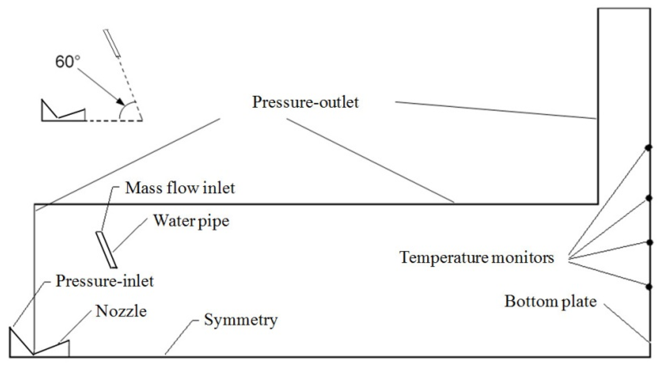
Figure 1 shows the computational domain and boundary conditions. Four temperature monitoring points on the bottom plate are marked. The distances of those points to the symmetry axis are 0.2, 0.3, 0.4 and 0.5 m, respectively. The angle between the water pipe and the symmetry axis is 60°. Because of the symmetry of jet flow, a quarter of three-dimensional computational domain is used to solve the flow field. This model is suitable for both two-pipe case and four-pipe case.

Figure 1. Schematic of the boundary condition.

Figure 1. Schematic of the boundary condition.

The nozzle wall, water pipes’ walls, and bottom plate are set as solid walls. The inlet boundary type of the nozzle is pressure inlet, and chamber pressure is 7 MPa, and temperature is 3000 K. The outlet boundary type of the plume is pressure outlet boundary, pressure is 1 bar, and temperature is 300 K. The mass flow rate of the rocket motor Q_g is 1.5 kg/s, which is invariable. The velocity of the combustion gas at the exit plate of the nozzle V_g is invariable, which is 2200 m/s. The outlet water velocity, number of pipes, and total mass flow rate of water pipes are variable in different cases.

3.2. Grid Independence

In transient numerical simulation, grid size and density directly have an effect on the accuracy of numerical calculations. Verifying the independence of grid is necessary before calculation. In this study, eight kinds of models with different grid sizes and densities are simulated. These models are divided into 100 thousand, 350 thousand, 600 thousand, 850 thousand, 1100 thousand, 1600 thousand, 2100 thousand and 2600 thousand grids, respectively. 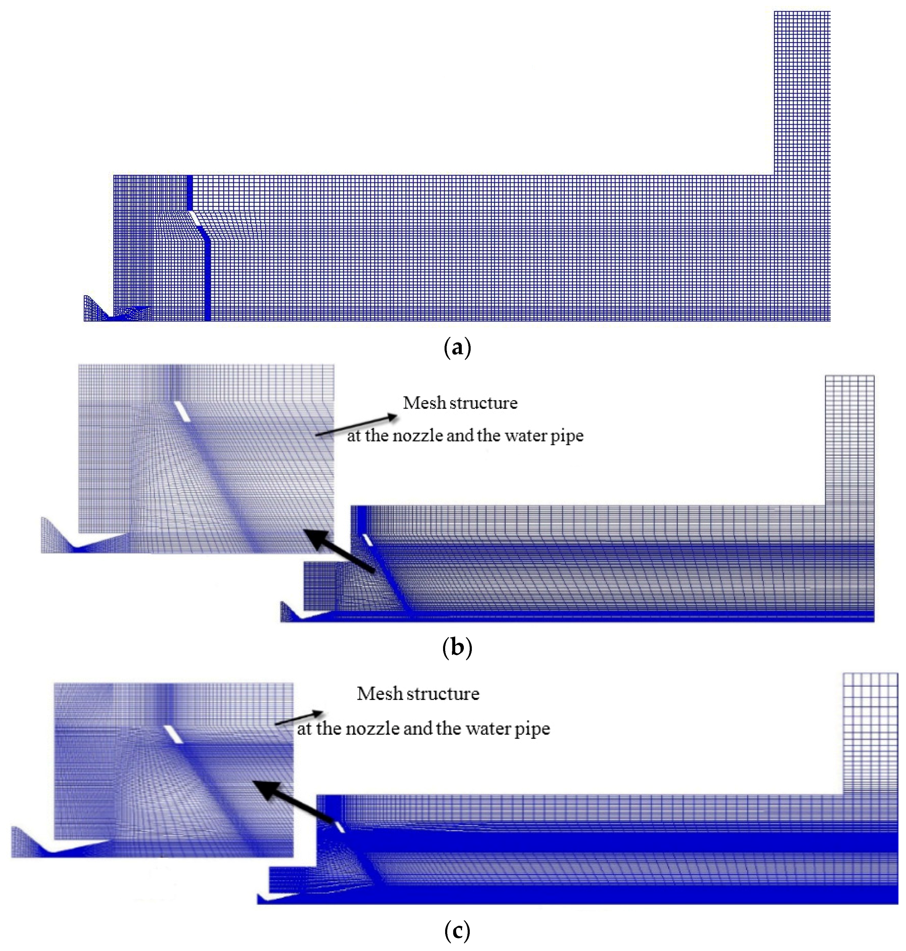In Figure 2, there are 600 thousand grids in Model A, 1100 thousand grids in model B, 2600 thousand grids in model C. By refining the grids in gas flow zone and zone nearby water pipe, the simulation results are close to the experimental results.

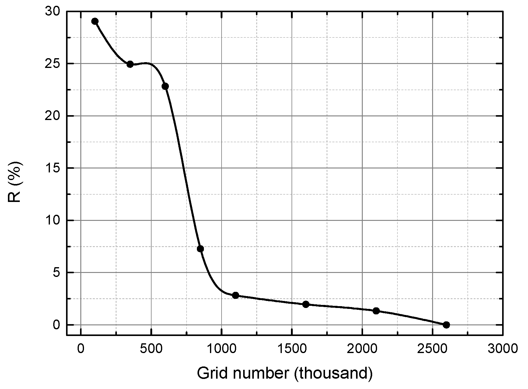
The two-phase flow coupled interaction is closely related to temperature in this study. By comparing the temperature, the appropriate grid size is determined. In Figure 3, the dimensionless temperature difference ratio is R:

$$R=\left|\left(T_C-T_{other}\right)/T_C\right|$$

(17)

where T_C is the temperature at the center of the bottom plate in model C and T_other is the temperature at the center of the bottom plate in other models. The difference ratio decreases with increasing grid number and then tends to be slow. The ratio is within 3% in the 1100 thousand, 1600 thousand and 2100 thousand grids models.

Figure 2. Mesh structure at the symmetry plane of the missile model. (a) Model A; (b) Model B; (c) Model C.

Figure 2. Mesh structure at the symmetry plane of the missile model. (a) Model A; (b) Model B; (c) Model C.

Figure 3. Dimensionless temperature difference ratio curve.

Figure 3. Dimensionless temperature difference ratio curve.

On account of the different grid sizes in these models, the temperature differences are compared in Figure 3. The Peclet number can be taken to explain the grid partitioning. It is a dimensionless number. It is defined to be the ratio of the rate of convection of a physical quantity by the flow to the rate of diffusion of the same quantity driven by an appropriate gradient. In 1976, Roache put forward the non-dimensional cell Peclet number as a measure of the relative strengths of convection and diffusion (Equation (18)) [19]:

$$Pe=\mathrm{\rho }u/\left(\mathrm{\Gamma }/\mathrm{\delta }x\right)$$

(18)

where u is the local flow velocity and δx is the cell width. ρ is the density. Γ is a constant relevant to flow field physical property on the compute node. Pe is proportional to δx. When Pe is greater than 1, convection is superior to diffusion and the calculation result is greatly influenced by the upstream node. Otherwise, diffusion is superior to convection and the calculation result is greatly influenced by the downstream node.

In this numerical calculation, u nearby the bottom plate is very small. With small δx the diffusion-dominated flow has a more accurate numerical result. The errors by numerical calculation in models with small grid size and refined grids are less than that in other models.

Also, the computing efficiency in the 1600 thousand, 2100 thousand and 2600 thousand grids models is about two-thirds of that in model B, so the 1100 thousand grid model was chosen for numerical calculation.

3.3. Numerical Method

The finite volume method was used to discretize the governing equations. The RNG k − ε model was used, as it is more accurate and reliable for a wider class of flows than the standard k − ε model. The adiabatic standard wall function was chosen for the working time of the engine. With coupling calculation, the energy source items were applied to the mixture model by UDF (User Defined Function) in gas-liquid multiphase flow filed.

4. Comparisons between Experiment and Simulation

4.1. Experiment System

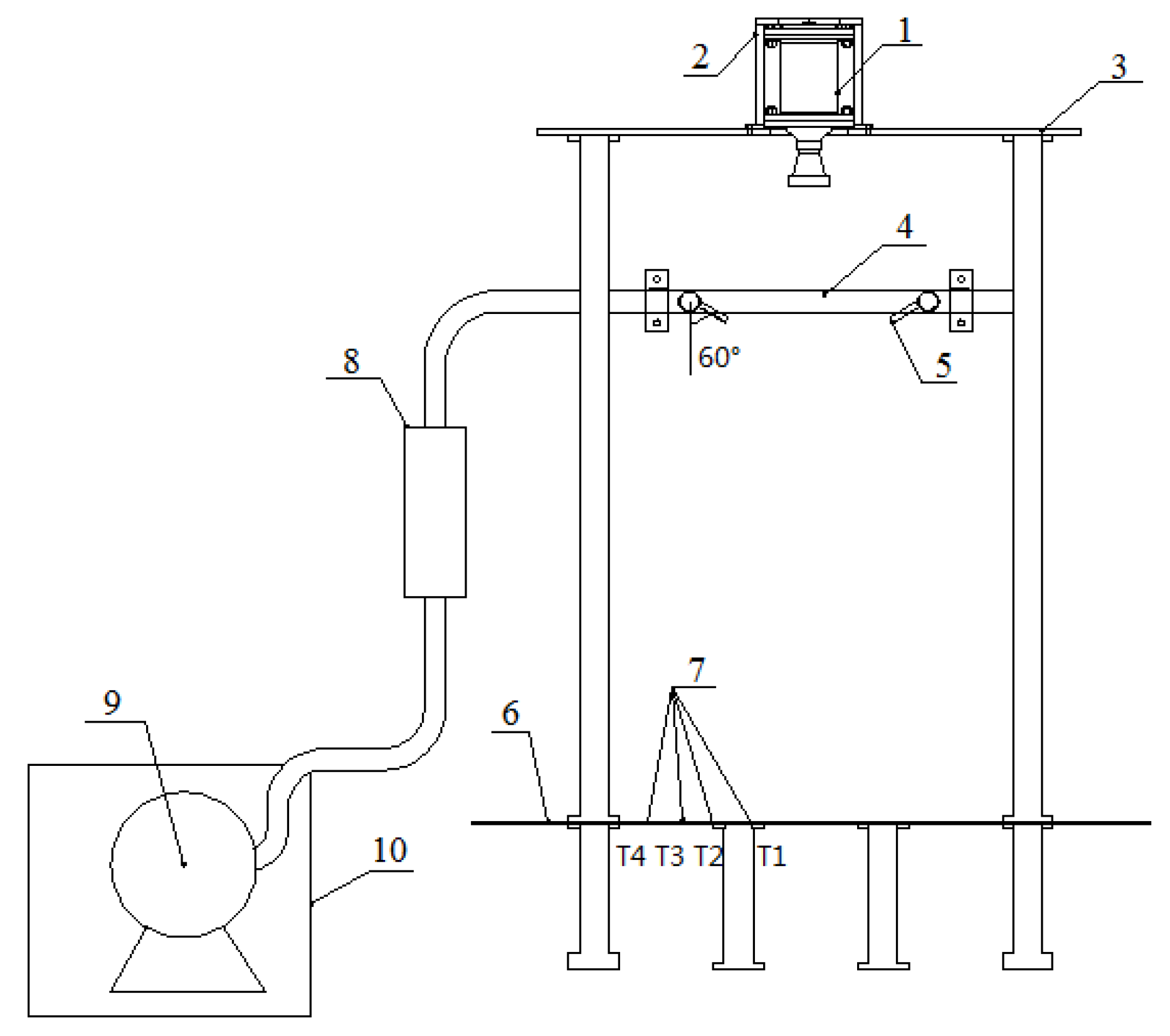
The schematic of the experimental system is shown in Figure 4. Water was supplied by a water pump to ensure constant water pressure. The mass flow rate was measured by a flow meter.

Figure 4. Schematic of the experiment system. 1. Rocket motor; 2. Engine mount; 3. Mounting plate; 4. Water pipe; 5. Pipe nozzle; 6. Testing bench; 7. Monitoring points (T1/T2/T3/T4); 8. Flow meter; 9. Pump; 10. Water box.

Figure 4. Schematic of the experiment system. 1. Rocket motor; 2. Engine mount; 3. Mounting plate; 4. Water pipe; 5. Pipe nozzle; 6. Testing bench; 7. Monitoring points (T1/T2/T3/T4); 8. Flow meter; 9. Pump; 10. Water box.

The angle between the water pipes (two or four pipes were chosen in different cases) and the centerline axis is 60°. The distance between the point of intersection of the centers of two water-injection pipes and that of nozzle exit is 520 mm. The temperature of the water injection is 300 K and water flow velocity is 16 m/s. The diameter of the round pipe is constant and equal to 12 mm. Four temperature sensors were fixed to the bottom plate of the bench to monitor the temperature. The locations of these sections are shown in Figure 4. An XSJ flow totalizer (Shanghai MeiKai YouDi Instrument Co., Shanghai, China) was employed for flow measurements. In addition to this contact measurement, non-contact measurement was chosen to detect the characters of the multiphase flow field by high-speed camera and infrared thermograph. To capture clearer images from the highly unsteady interaction between the water and combustion gas, a Phantom v10 high-speed camera and TVS2000 (NEC-AVIO Co., Tokyo, Japan) infrared thermograph were used to observe the flow field structure and the radiation intensity emitted from the exhaust plume. The sampling frequency of the Phantom v10 high-speed camera is 480 images/s and the resolution of the images is 2400 × 1800 pixels. The resolution and the sampling frequency of the TVS2000 infrared thermograph is 0.1 °C and 30 images/s. The E12-1-C-U temperature sensors (Nanmac Co., Washington, DC, USA) are used to monitor the temperature of the four points. The measuring limit of E12-1-C-U temperature sensor is 3300 K, which could satisfy the demands of exhaust plumes temperature test.

A horizontal motor test bench is generally selected for the engine test, as it is easy to design and assures testing security. However, in consideration of the large mass of water, which may result in much more gravitational influence, a vertical test bench is chosen to simulate the rocket launching more truly. Furthermore, a vertical motor test bench makes the measurements more accurate and the test equipment such as high-speed camera and infrared thermograph is more easily located.

Too high an experiment mounting plate tends to render the entire device unsteady. Too low an experiment mounting plate makes it difficult to perform a complete observation. In this study, the height of the mounting plate depends on the length of the core region of the jet:

$$\frac{x}{r_e}=6.9{\left(1+0.38Ma\right)}^2$$

(19)

where x is the length of the core region; r_e is the radius of nozzle exit; Ma represents Mach number and equals 3.5 in this study.

Calculated according to this formula [20], the length of the core region is 1.33 m. The simulation results show that the length of the core region is between 1.25 and 1.4 m. The simulation confirms the effectiveness of Equation (19). Then, considering the length of the motor nozzle, the height of the mounting plate is 1.9 m.

To simulate typical rocket exhaust conditions, the designed Mach number of the free jet in the test is about 3.5 and the outlet temperature is approximately 2000 K. To realize this condition, a solid rocket motor was chosen. The total temperature and total pressure of the combustion chamber are 3000 K and 7 MPa, respectively. The jet flow of this rocket motor is an axisymmetric over-expanded flow, so the rocket motor is designed based on the basic formula of one-dimensional isentropic flow and the combustion characteristic of solid motor grain. The rocket motor is shown in Figure 5.

Figure 5. Rocket motor.

Figure 5. Rocket motor.

With composite modified double base propellant, the screw-compressed motor grain is available. To ensure a steady thrust, the combustion of internal propellant occurs simultaneously with the external propellant, and both sides of the motor grain are covered by flame-resistant material under constant temperature and pressure.

4.2. Free Jet without Water Injection

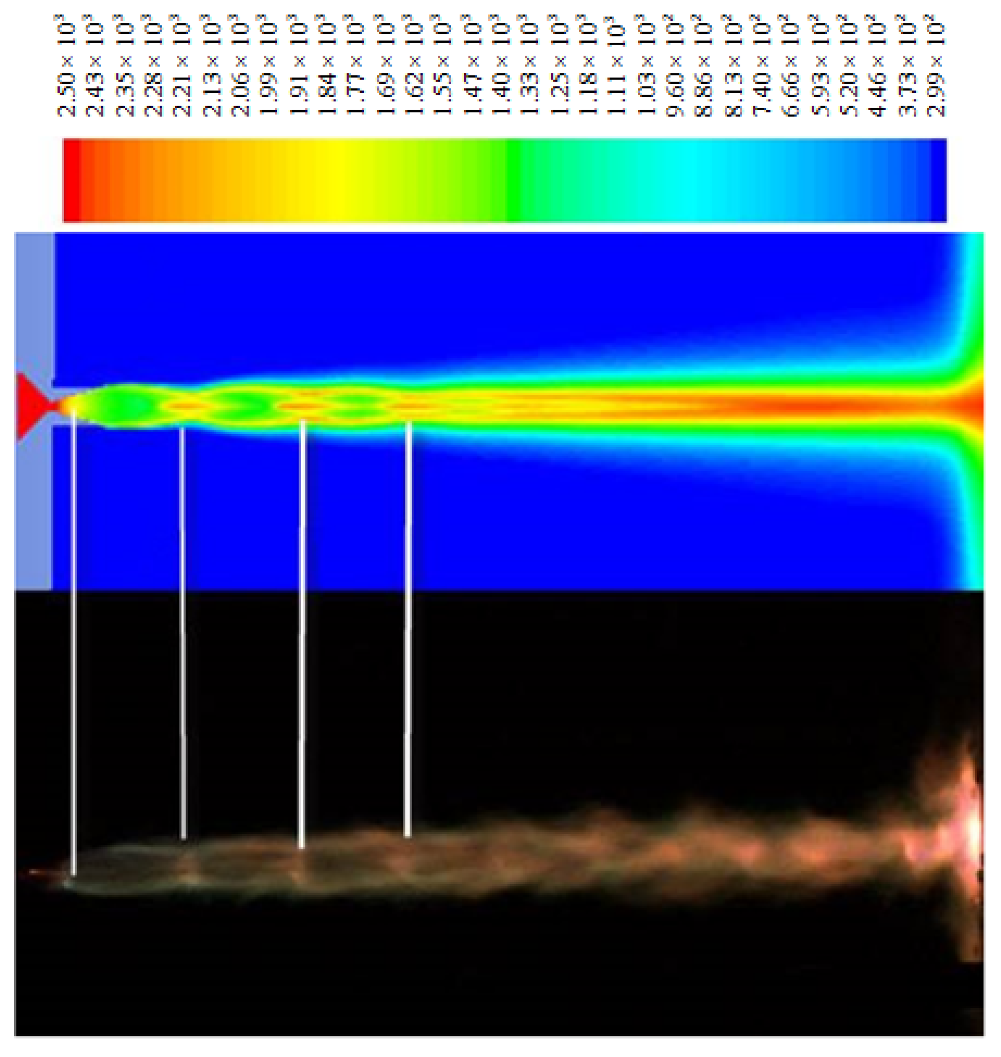
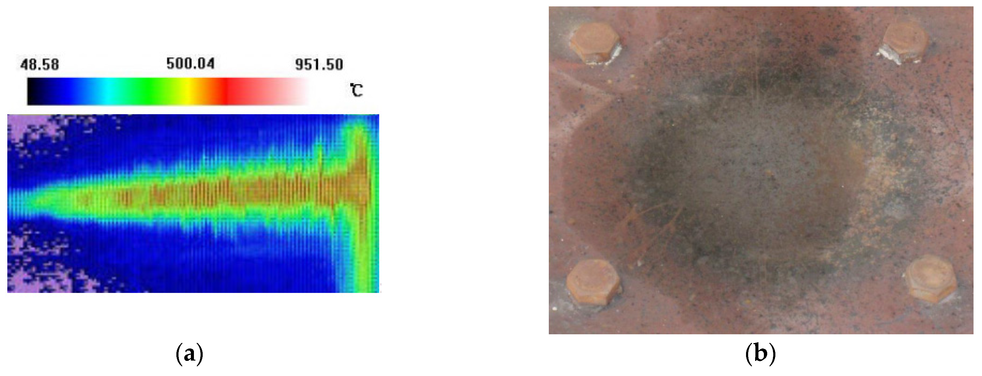
As shown in Figure 6, two photographs were taken under the combustion steady process conditions. With the over-expanded nature of the jet, five shock cells are clearly seen in the jet core region of free jet flow in. The location of first shock cell is x₁ = 2.1 d_e, and the location of the second one is x₂ = 4.9 d_e. The temperature in IR image ranges from 0 to 1000 K (Figure 7a). The flow pattern of free jet in high-speed camera and infrared thermograph resemble each other, especially the high-temperature core region, which extends from the exit to the bottom plate.

Figure 6. Free jet without water injection.

Figure 6. Free jet without water injection.

Figure 7. (a) IR (Infrared Radiation) image; (b) Picture of erosion region.

Figure 7. (a) IR (Infrared Radiation) image; (b) Picture of erosion region.

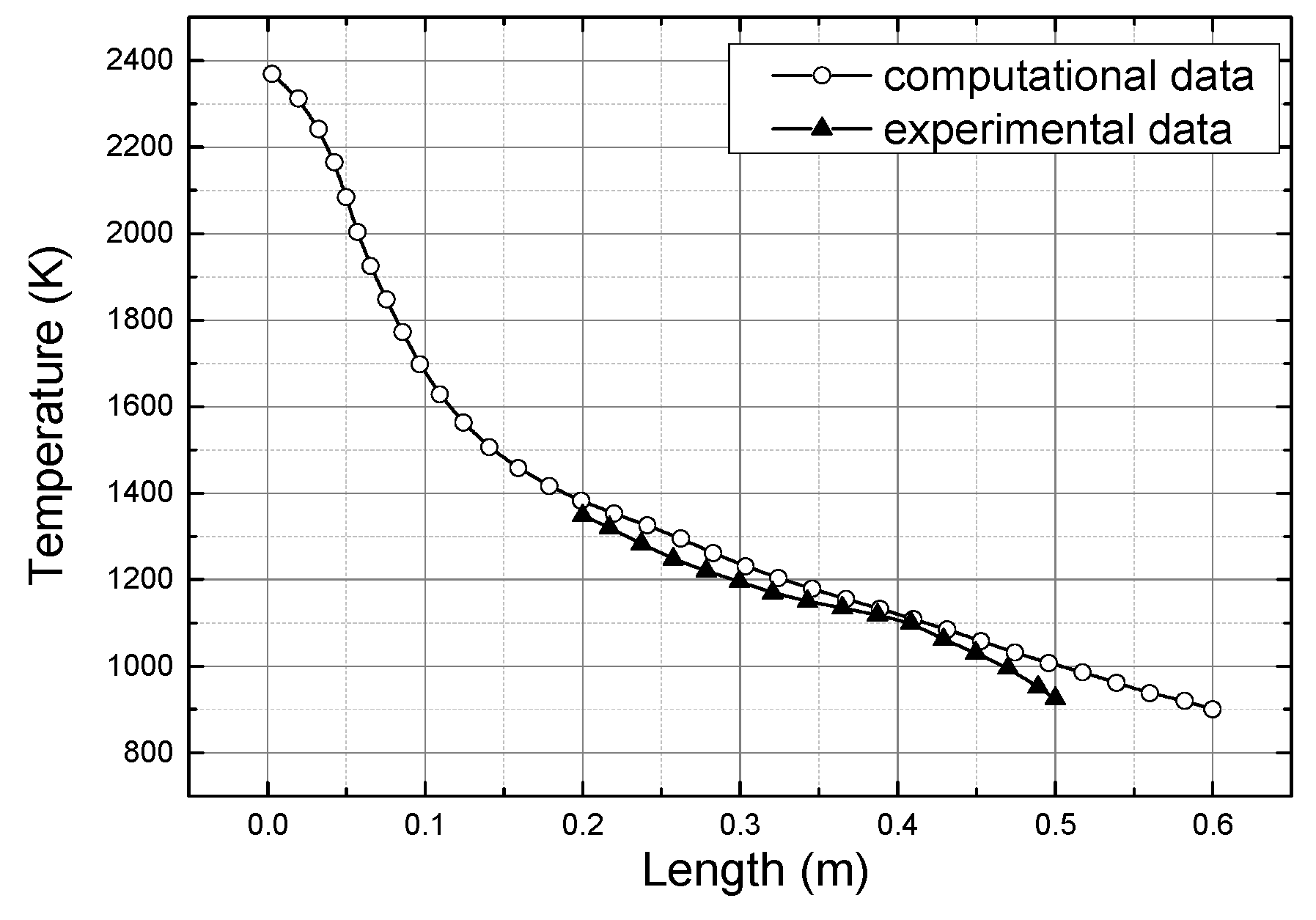
As shown in Figure 6 the high-speed photograph is in accordance with the predicted temperature contour. Moreover, the same number of clear Mach disks is noted. Temperature distribution without water injection is clearly displayed and the temperature of central line is the highest. The temperatures of the testing bench from experiment and that in simulation are consistent with each other in Figure 8. The peak temperature at the center point of the testing bench reaches 2400 K. The monitoring point that is 0.2 m from the center of the testing reaches up to about 1350 K. Obviously, there is extreme shock and ablation on the testing bench owing to the free jet (Figure 7b).

Figure 8. Comparison chart of monitor values and computational values.

Figure 8. Comparison chart of monitor values and computational values.

4.3. Jet with Water Injection

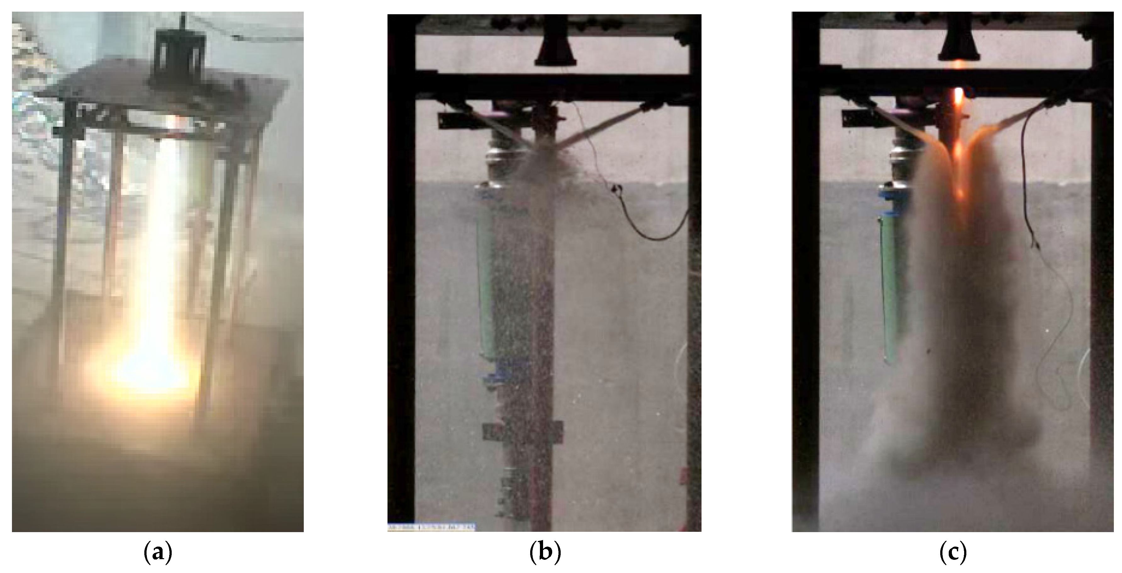
The conditions for simulation are the same as those for the experiments. The photos given are digital video images and high-speed photographs. The flat deflector plate was shocked by jet flow without water to cause the plate to be seriously ablated in Figure 9a. As shown in Figure 9b, jets flowing symmetrically from two pipes intersected directly under the engine nozzle, spraying small drops of water all around. A large amount of water vapor began to be produced after injecting water into the jet flow in Figure 9c.

Figure 9. (a) Jet flow model without water; (b) Water injection model without jet flow; (c) Water injection model with jet flow.

Figure 9. (a) Jet flow model without water; (b) Water injection model without jet flow; (c) Water injection model with jet flow.

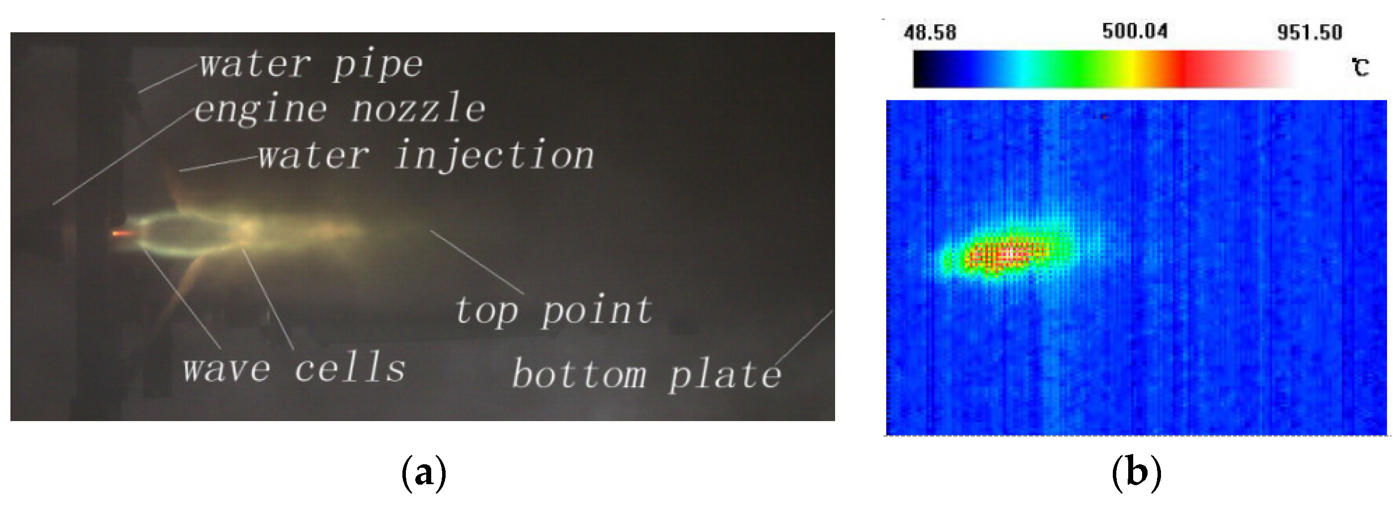
There are only two shock cells, which are clearly visible in Figure 10a for the water injection. It is easy to find that the first shock cell is at the same location as the case without water injection $\dot{x_1}=2.1d_e$. However, the interaction between the water spray and the main supersonic combustion gas stream is highly unsteady, so the second one is not fixed as the impact of the water injection, $\dot{x_2}$ varied between 4.7d_e and 5.1d_e. The jet core region is compressed to an isosceles triangle, the peak of which is not stable and the apex angle varied rapidly between 0.5β and 1β. β = 15° is expansion cone half angle. The shape of the jet core region shown in IR (Infrared Radiation) image is similar to that shown in Figure 10b.

Figure 10. (a) High-speed photograph; (b) IR image.

Figure 10. (a) High-speed photograph; (b) IR image.

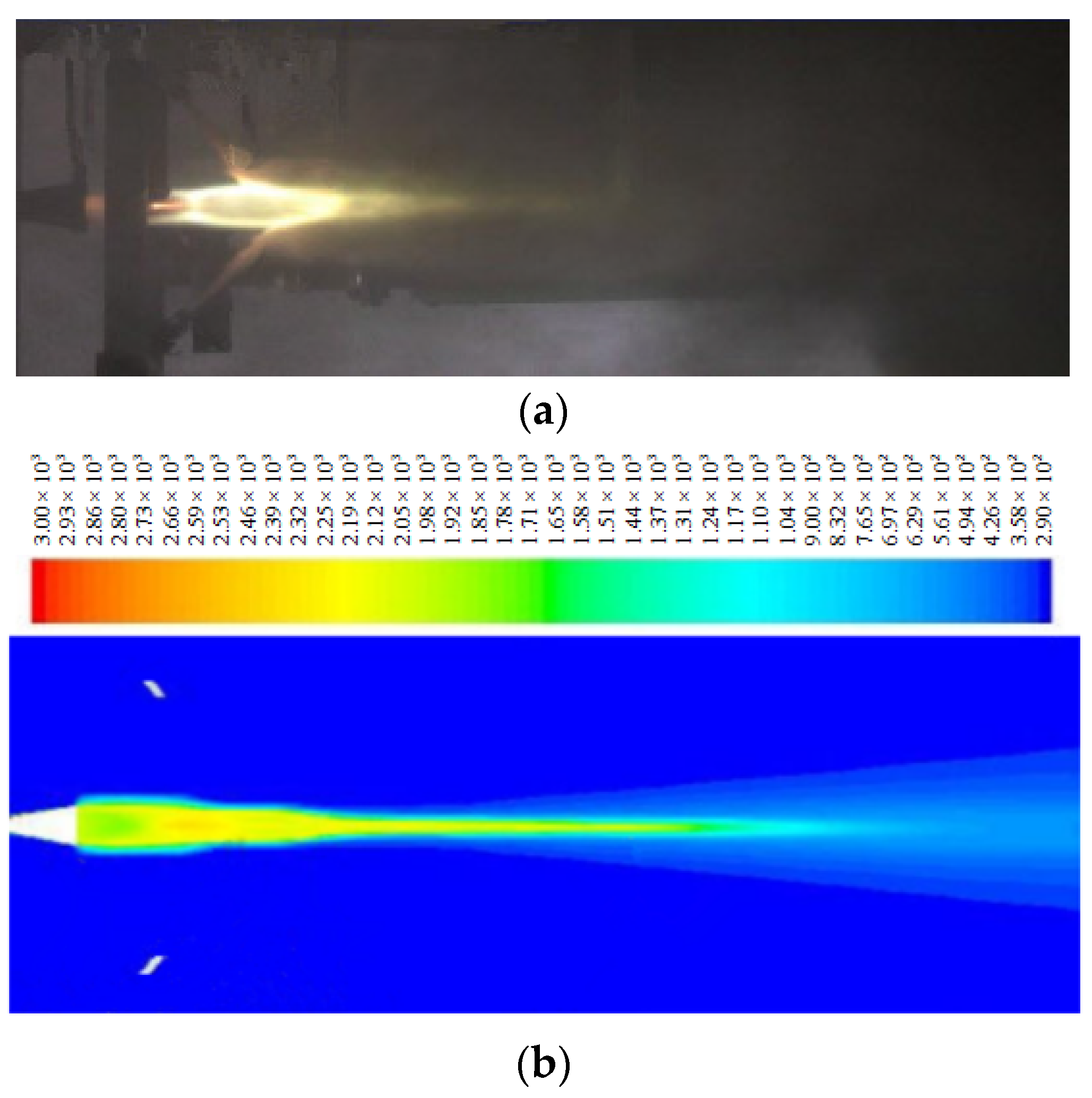
In experiment and simulation, mass flow rate of each water pipe is Q_w = 1.8 kg/s and mass flow rate of jet is Q_g = 1.5 kg/s. Outlet water velocity is 16 m/s and there are two pipes. Because of the water injection, the length of the jet core region in the state of water injection is shorter than that of free jet (Figure 11). The jet flow shape and temperature distribution is consistent in the two pictures.

Figure 11. (a) Experimental jet with water injection; (b) Temperature contour with water injection.

Figure 11. (a) Experimental jet with water injection; (b) Temperature contour with water injection.

Moreover, the numerical results agree well with the experimental results at monitoring points (Table 1). The maximum error between the two results is within 10%. Through comparison of data and temperature-distribution pictures between the experiments and simulations, the simulation model is suitable for verifying the experiment.

Table 1. Comparison between experimental data and numerical data.

Monitoring Point	T1	T2	T3	T4
Experimental average temperature (K)	471.3625	420.3750	460.2618	413.5852
Numerical average temperature (K)	451.3773	432.4919	414.6886	400.3756
Error (%)	4.23	−2.88	9.90	3.19

Table 1. Comparison between experimental data and numerical data.

Monitoring Point	T1	T2	T3	T4
Experimental average temperature (K)	471.3625	420.3750	460.2618	413.5852
Numerical average temperature (K)	451.3773	432.4919	414.6886	400.3756
Error (%)	4.23	−2.88	9.90	3.19

4.4. Temperature Comparison

As shown in Figure 12a, the total temperature of free jet is compared with that of jet with water injection in the plane-XOY. The temperature comparison between free jet and jet with water injection in the plane-XOZ is shown in Figure 12b. The X-axis is vertical axis of the nozzle. The plane of two water pipes is named plane-XOY and its perpendicular plane is named plane-XOZ.

Figure 12. (a) Temperature comparison between free jet and jet with water injection in the XOY plane; (b) Temperature comparison between free jet and jet with water injection in the XOZ plane.

Figure 12. (a) Temperature comparison between free jet and jet with water injection in the XOY plane; (b) Temperature comparison between free jet and jet with water injection in the XOZ plane.

The external zone of the jet with injected water is a subsonic one, but the internal zone is a supersonic one, so the influence of water on external zone is greater than that on internal zone. The length of flow core region is shortened by injecting water. The energy of the core region hardly transmits outward through heat transfer means that the temperature distribution of the free jet is similar to that of the jet with water injection near the X-axis. The diameter of the pipe is constant and two pipes are only installed in the XOY plane. The location of pipes causes jet asymmetry, so the interphase interaction between liquid and gas in the XOZ plane decreases and the temperature distribution of the flow is wider when compared with that of the XOY plane.

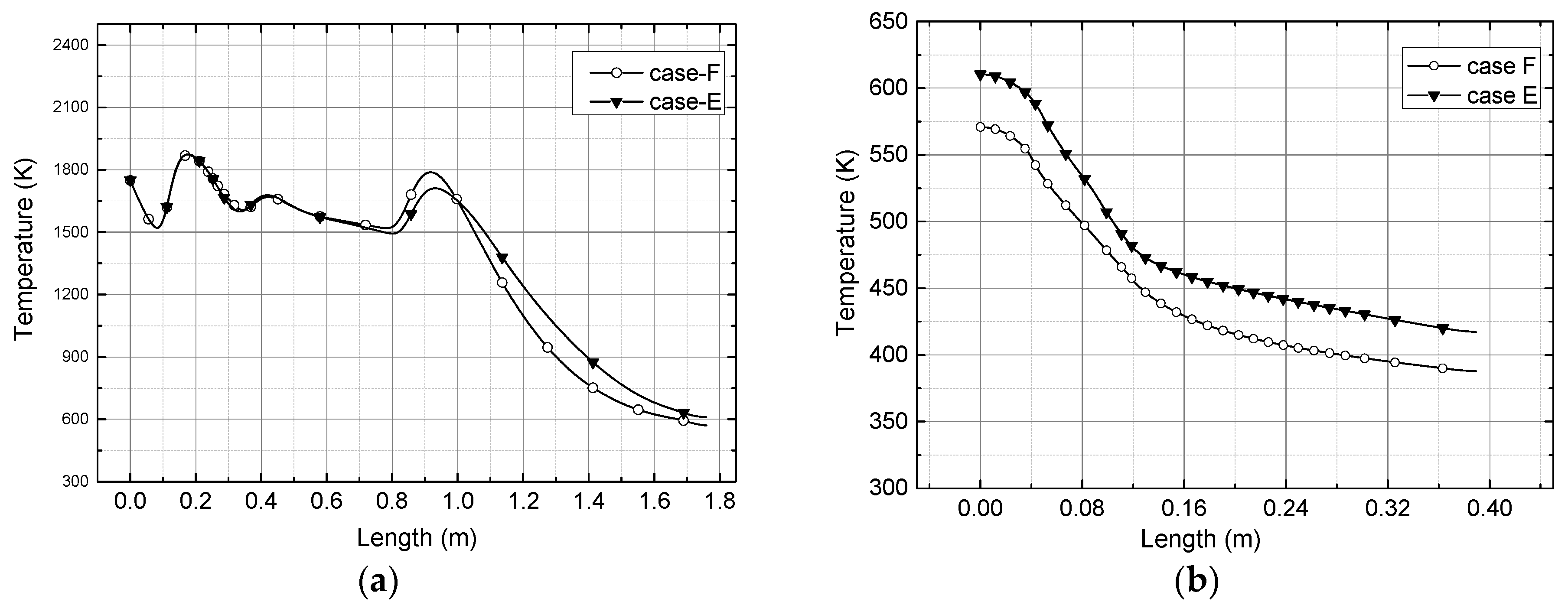
The axial temperature of jet flow shows a serious decrease in the second half of the flow in Figure 13a. The point A is the water injection location on the X-axis. This point and the nozzle exit are 0.592 m apart. The maximum temperature of the axial temperature exhibits two peaks. The first one is located at the same place as in the free jet case; the second one lies on the place of 0.75 m of distance from the exit plate, which is the apex of an isosceles triangle jet core. The temperature decreased rapidly after the second peak value due to the endothermic water vaporization process. The maximum reduction of temperature is nearly 70% of the free jet case and the mean reduction of temperature is about 50% in the center line. The predicted average temperature at the central line of the jet core region illustrates that the cooling effect is obvious. This is clearly reported by infrared thermography and the temperature contour.

Figure 13. (a) Axial temperature; (b) Temperature of the testing bench.

Figure 13. (a) Axial temperature; (b) Temperature of the testing bench.

The temperature of the bench without water is shown as a line-free in Figure 13b. In the case with water injection, line Y is parallel to the XOY plane and line Z is parallel to XOZ plane. There is an interesting phenomenon that the monitoring line temperature of line Z is slightly below that of line Y (Figure 13b). The reason is that the contact area between water and the expanded jet flow without water shock is great. The energy loss increases with more vaporization than that of the XOZ plane. The monitoring point temperature of the flow center is about 480 K and is down to 20%. The monitoring point temperature at 0.2 m drops to 34.6%. The average temperature of the bench is 100–200 K. It is concluded that the effect of cooling in the surrounding places as well as that in the center and the temperature distribution of the bottom plate does produce a drastic change like the free jet case.

5. Results and Analysis

Table 2 shows different cases of water injection considered. The cooling effects caused in the various conditions are shown below.

Table 2. Computational cases.

Parameter/Result	A	B	C	D	E	F
Mass flow rate of each water pipe Qw (kg/s)	3	3	3	7.2	1.31	2.06
Mass flow rate of jet (kg/s)	1.5	1.5	1.5	1.5	1.5	1.5
Outlet water velocity (m/s)	7.5	12	17.05	37	5.85	9.18
Number of pipes	2	2	2	2	4	4

Table 2. Computational cases.

Parameter/Result	A	B	C	D	E	F
Mass flow rate of each water pipe Qw (kg/s)	3	3	3	7.2	1.31	2.06
Mass flow rate of jet (kg/s)	1.5	1.5	1.5	1.5	1.5	1.5
Outlet water velocity (m/s)	7.5	12	17.05	37	5.85	9.18
Number of pipes	2	2	2	2	4	4

5.1. Effect of Water Injection Velocity

Cases A, B, C and D have the same mass flow rate and pipe number but different velocities. Figure 14a shows the vaporization rate in the four cases. The vaporization rate gradually rises and becomes stable, and in the stable stage, there is pulsating change periodically.

Figure 14. (a) Vaporization rate; (b) Mass of the remaining water; (c) Temperature of axial gas stream.

Figure 14. (a) Vaporization rate; (b) Mass of the remaining water; (c) Temperature of axial gas stream.

The vast amount of water vaporizes instantly impacting the main stream. The ratio of transient impulse changes and the contact area also changes between the gas phase and water phase. Then, the momentum ratio of the two phases is back to the initial one because of constant water resupply, so the vaporization ratio changes periodically. In cases A, B and C, the lower the water velocity is, the lower the vaporization rate is. However, the vaporization rate of case D is close to that of case B. The phenomenon is caused by the higher water velocity in case D. There are two branching flows in Figure 15, so the contact area decreases and vaporization rate is lower than that of case C. As shown in Figure 14b, the mass of remaining water does not change when the vaporization rate tends to be stable. The temperature along the jet axis decreases as the temperature decreases. It indicates that it is available to improve the efficiency of the vaporization rate by appropriately choosing the water velocity.

Figure 15. Temperature contour of the XOZ plane in case D.

Figure 15. Temperature contour of the XOZ plane in case D.

5.2. Effect of Water Mass Flow Rate

In Table 2, the water mass flow rate in case D is about 2.5 times more than that in case C, and mass flow rate of water in case E is lower than that in case F. It is obvious that cooling effect relates to this condition in Figure 15 and Figure 16. The temperature decreases with increasing mass flow rate.

Figure 16. (a) Temperature of axial gas stream; (b) Temperature of monitoring line.

Figure 16. (a) Temperature of axial gas stream; (b) Temperature of monitoring line.

5.3. Effect of Exhaust Jet Momentum

Table 3 shows that the vaporization rate in case H is the highest when compared with those in other cases. Before the formation of the two branching flows, the vaporization rate rises with increasing outlet water velocity, but after passing the tipping point, the vaporization rate gradually drops with increasing outlet water velocity.

The dimensional polylines between the momentum ratio and vaporization rate are based on Table 3. In Figure 17, the jet flow showa compressive deformation and two branching flows were formed in all simulations, so the polylines are in accordance with the relevant physical laws. With the same conditions except outlet water velocity, the best cooling effect appears on around momentum ratio 50.

Table 3. Computational results.

Parameter/Result	A	B	G	C	I
Mass flow rate of each water pipe Qw (kg/s)	3	3	3	3	3
Mass flow rate of jet (kg/s)	1.5	1.5	1.5	1.5	1.5
Outlet water velocity (m/s)	7.5	12	15	17.5	30
Number of pipes	2	2	2	2	2
Ratio of momentum (Mg/Mw)	88.14	55.08	44.07	38.88	22.03
Vaporization Rate (kg/s)	1.24	1.4	1.92	1.4	1.28
Ratio of vaporization rate (K)	0.667	0.729	1	0.729	0.646

Table 3. Computational results.

Parameter/Result	A	B	G	C	I
Mass flow rate of each water pipe Qw (kg/s)	3	3	3	3	3
Mass flow rate of jet (kg/s)	1.5	1.5	1.5	1.5	1.5
Outlet water velocity (m/s)	7.5	12	15	17.5	30
Number of pipes	2	2	2	2	2
Ratio of momentum (Mg/Mw)	88.14	55.08	44.07	38.88	22.03
Vaporization Rate (kg/s)	1.24	1.4	1.92	1.4	1.28
Ratio of vaporization rate (K)	0.667	0.729	1	0.729	0.646

Figure 17. Dimensional polylines between momentum ratio and vaporization rate.

Figure 17. Dimensional polylines between momentum ratio and vaporization rate.

6. Conclusions

This investigation addresses the concept of injecting water into the rocket exhaust plume to reduce the jet temperature. A series of experiments of injecting water into the exhaust plume, which were performed in a controlled laboratory environment, were run. A mixture multiphase model, which introduces the energy source items caused by the vaporization of liquid water into the energy equation, was developed to simulate the flow field of the complex gas-liquid multiphase flow. This multiphase model was validated by the experimental results. The flow field, distribution of temperature in both simulation and experiment, and cooling effect were discussed.

It is seen that the high temperature core region of the plume is compressed to an isosceles triangle by water injection in both the numerical simulations and experiments. The length and the area of the core are smaller than those of the free jet, respectively, especially the region whose temperature is higher than 1000 K. The main energy of the plume jet is concentrated up the high temperature core region, where it is feasible to cool the rocket exhaust plume by evaporation of water injection.

The stagnation temperature of the plume sometimes leads to damage of launcher structures due to high temperature erosion. As a result, the cooling effect on the bottom plate warrants further study. The stagnation temperature disappears in the center of the bottom plate for the water injection, and Figure 14 shows that the effect of cooling in the center is better, and the temperature distribution of the bottom plate departs considerably from the free jet case.

In the different cases considered, the varying parameters like mass flow rate, pipe number, and outlet water velocity can produce temperature distribution variations on the bottom plate. The momentum of water was chosen as an important parameter, which influences the cooling effect by comparative analysis. A scaling equation of a dimensionless relationship between reduction in mean temperature and momentum ratio is calculated to predict the cooling effect of subscale or full-scale launching test.

It should be noted that this study has not examined the cooling effect of the injection angle and the water injection orifice diameter. Further study is needed to investigate the effect of the variable multiphase flow field. Notwithstanding its limitations, this study does confirm that water injection is an effective coolant for rocket motor exhaust. At the same time, a preliminary study of the mechanism of the interaction of water and combustion gas and the relationship between cooling effect and the momentum ratio were developed, which could be used to predict the results in a full-scale launch test.

References

- Giordan, P.; Fleury, P.; Guidon, L. Simulation of water injection into a rocket motor plume. In Proceedings of the 35th Joint Propulsion Conference and Exhibit, Los Angeles, CA, USA, 20–24 June 1999.
- Marchesse, Y.; Gervais, Y.; Foulon, H. Water injection effects on hot supersonic jet noise. Compt. Rend. Mec. 2002, 330, 1–8. [Google Scholar] [CrossRef]
- Golden, D.; Cerza, M.; Myre, D. An experimental study of water injection into a Rolls-Royce model 250-C20B turboshaft gas turbine. In Proceedings of the 44th Joint Propulsion Conference and Exhibit, Hartford, CT, USA, 21–23 July 2008.
- Mathias, E.; Born, S. Cooling system for the statically tested space shuttle full-scale solid rocket motors. In Proceedings of the 25th Joint Propulsion Conference, Monterey, CA, USA, 10–12 July 1989.
- Miller, M.J.; Koo, J.H. Effect of water to ablative performance under solid rocket exhaust environment. In Proceedings of the 29th Joint Propulsion Conference and Exhibit, Monterey, CA, USA, 15–18 November 1993.
- Santangelo, P.J.; Kennedy, I.M. An experimental study of droplet dynamics in a turbulent droplet-laden round jet. In Proceedings of the 35th Aerospace Sciences Meeting and Exhibit, Reno, NV, USA, 9 January 1997.
- Engblom, W.A.; Fletcher, B.; Georgiadis, N.J. Validation of conjugate heat-transfer capability for water-cooled high-speed flows. In Proceedings of the 39th American Institute of Aeronautics Astronautics Thermophysics Conference, Miami, FL, USA, 25–28 June 2007.
- Kandula, M. Prediction of turbulent jet mixing noise reduction by water injection. AIAA J. 2008, 46, 2714–2722. [Google Scholar] [CrossRef]
- Cho, C.S.; Gerald, A.P. Effect of coolant injection to small-scale diffuser simulating SSME testing conditions. In Proceedings of the 38th Joint Propulsion Conference and Exhibit, Indianapolis, IN, USA, 7–10 July 2002.
- Washington, D.; Krothapalli, A. The role of water injection on the mixing noise supersonic jet. In Proceedings of the 4th AIAA/CEAS (American Institute of Aeronautics Astronautics/Confederation of European Aerospace Socirties) Aeroacoustics Conference, Toulouse, France, 2–4 June 1998.
- Krothapalli, A.; Venkatakrishnan, L.; Lourenco, L. Supersonic jet noise suppression by water injection. In Proceedings of the 6th Aeroacoustics Conference and Exhibit, Lahaina, HI, USA, 12–14 June 2000.
- Brenton, G.; Anjaneyulu, K. Jet noise reduction using aqueous microjet injection. In Proceedings of the 10th AIAA/CEAS (American Institute of Aeronautics Astronautics/Confederation of European Aerospace Socirties) Aeroacoustics Conference, Manchester, UK, 10–12 May 2004.
- ANSYS Fluent Theory Guide; ANSYS, Inc.: Canonsburg, PA, USA, 2013; pp. 373–502.
- Wen, C.Y.; Yu, Y.H. Mechanics of fluidization. Chem. Eng. Prog. Symp. 1966, 62, 100–111. [Google Scholar]
- Lee, W.H. A pressure iteration scheme for two-phase flow modeling. In Proceedings of the IEEE Engineering in Medicine and Biology Society Annual Conference, Washington, DC, USA, 28 September–30 October 1980; pp. 407–427.
- Yuki, K.; Abei, J.; Hashizume, H.; Toda, S. Numerical investigation of thermofluid flow characteristics with phase change against high heat flux in porous media. J. Heat Transf. 2008, 130, 73–84. [Google Scholar] [CrossRef]
- He, G.; Yamazaki, Y.; Abudula, A. A droplet size dependent multiphase mixture model for two phase flow in PEMFCs. J. Power Sources 2009, 194, 38–44. [Google Scholar] [CrossRef]
- Ma, Y.; Jiang, Y. Research on launching process cooling effect of wet concentric canister launcher. J. Ballist. 2010, 22, 89–93. [Google Scholar]
- Computational Fluid Dynamics; ANSYS, Inc.: Canonsburg, USA, 2007; pp. 143–144.
- Hu, F.; Zhang, W.; Xiang, M.; Huang, L. Experiment of water injection for a metal/water reaction fuel ramjet. J. Propul. Power 2008, 29, 686–691. [Google Scholar] [CrossRef]
© 2015 by the authors; licensee MDPI, Basel, Switzerland. This article is an open access article distributed under the terms and conditions of the Creative Commons by Attribution (CC-BY) license (http://creativecommons.org/licenses/by/4.0/).