Power Management Strategy of Hybrid Electric Vehicles Based on Quadratic Performance Index

Abstract

An energy management strategy (EMS) considering both optimality and real-time performance has become a challenge for the development of hybrid electric vehicles (HEVs) in recent years. Previous EMSes based on the optimal control theory minimize the fuel consumption, but cannot be directly implemented in real-time because of the requirement for a prior knowledge of the entire driving cycle. This paper presents an innovative design concept and method to obtain a power management strategy for HEVs, which is independent of future driving conditions. A quadratic performance index is designed to ensure the vehicle drivability, maintain the battery energy sustainability and average and smooth the engine power and motor power to indirectly reduce fuel consumption. To further improve the fuel economy, two rules are adopted to avoid the inefficient engine operation by switching control modes between the electric and hybrid modes according to the required driving power. The derived power of the engine and motor are related to current vehicle velocity and battery residual energy, as well as their desired values. The simulation results over different driving cycles in Advanced Vehicle Simulator (ADVISOR) show that the proposed strategy can significantly improve the fuel economy, which is very close to the optimal strategy based on Pontryagin’s minimum principle.

1. Introduction

As increasingly concerning on the deterioration in air quality and decrease in petroleum resources, a great interest is shown in the development of safe, clean, and high-efficient transportation. It has been well recognized that the electric vehicle (EV), hybrid electric vehicle (HEV), and fuel cell electric vehicle (FCEV) are the most promising solution to the problem of land transportation in the future [1]. Since showing improvement in fuel consumption with minimum extra cost, HEVs are considered to offer the best promise in the short to mid-term [2]. In HEVs, the internal combustion engine (ICE) provides driving power together with one or more reversible energy storage systems (ESSes), such as a bank of batteries and ultra-capacitors, which are generally used as an energy buffering unit to recycle braking energy and change engine operating points as well as provide an extra degree of freedom for energy management strategies (EMSes). Undeniably, the introduction of ESSes makes driving modes more flexible but EMSes more complicated. Therefore, it is especially important to design an excellent EMS for HEV development and application [3,4].

As early as 1997, Jalil used a set of predefined rules based on the battery state of charge (SOC) and power demand to assign the power to the engine, battery, or a combination of both, for a series HEV to ensure the high efficiency of the engine and battery operation [5]. Such rule-based strategies developed from heuristic ideas are widely used in HEVs [6,7,8] because they can be implemented in real-time, but making rules commonly depends on engineering experience, known mathematical models, large numbers of experimental results, etc., having limited benefits for fuel economy. In order to improve the fuel economy of rule-based methods, Schouten and Duan directly adopted fuzzy rules instead of deterministic ones to improve the operation efficiency of vehicle system in 2002 and 2003 [9,10]. Zhao added a fuzzy algorithm to modify the rules in 2013 [11]. However, the fuel-saving potential of HEVs cannot be fully exploited because the membership functions and rules of a fuzzy controller are designed based on human expertise and heuristics. To further reduce fuel consumption, fuzzy controllers were modified by offline optimizing membership functions and rules through a particle swarm optimization algorithm [12], a genetic algorithm [13], or a machine learning algorithm [14]. Alternatively, a learning vector quantization neural network [15] or a fuzzy neural network [16] is used in a fuzzy EMS to identify the driving cycle style periodically.

By contrast with above heuristic-based strategies, EMSes based on optimal control theory, such as dynamic programming (DP) and Pontryagin’s minimum principle (PMP) have been investigated quite intensively in recent years. For a prior known driving cycle, DP discretizes continuous states and control values into finite grids and decomposes the overall dynamic optimization problem into a sequence of sub-problems. The cost function of each sub-problem is the fuel consumption from current step to last step. By calculating backwards along the horizon based on Bellman’s Principle of Optimality, DP generated an optimal EMS of HEVs, but with a large computational load that exponentially increases as the state variables increase in number [17,18,19,20]. Theoretically, if the whole driving cycle is known in advance and the performance index is defined as an integral of fuel consumption rate, the EMS obtained from DP will minimize the total fuel consumption. However, such an optimal solution is only suitable for the known driving cycle rather than other ones. The requirement for future driving demands to be known in advance leads to a real-time problem, so DP always acts as a benchmark to assess other EMSs [21,22]. To apply the optimal results of DP in real-time, many attempts have been made, such as extracting rules from optimal results [23,24], modeling the power demand as a random Markov chain [25,26] or predicting future driving conditions [27,28,29].

As another popular theory-based method, PMP formulates the optimal control problem of HEVs as a two-point boundary value problem of nonlinear differential equations. In this method, the whole driving cycle still needs to be known in advance but the computation load is much less than DP [30]. A study on the comparison between PMP and DP demonstrated that the optimal results generated by PMP are very close to DP [31], so PMP can also be a benchmark. Furthermore, Kim, Cha, and Peng had proved in 2011 that under the assumption that the battery SOC varies within a small range, the Lagrange multiplier $\text{λ}$, which is also called as a co-state, is a constant [32]. On the other hand, $\text{λ}$ can be interpreted as an equivalent factor to equate the electrical usage of a battery to virtual fuel consumption. When $\text{λ}$ is a constant, the dynamic optimization problem is converted into a static one, and the equivalent consumption minimization strategy (ECMS) is developed [33,34]. However, $\text{λ}$ is still very sensitive to driving cycles. Much work has been reported to solve the above problem, such as developing a function to estimate equivalent factors through observing a number of optimal results calculated from DP and PMP [35], designing a driving cycle recognizer using a neural adaptive network [36], or adding an online algorithm to ECMS framework to periodically refresh equivalent factors combined with the past and predicted vehicle speed and GPS data [37]. However, if these modified theory-based methods are applied to real vehicles, they are sub-optimal, complex, and time-consuming.

In summary, the rule-based strategies are suitable for real-time applications but with limited fuel economy while the optimal theory-based strategies have the real-time problem caused by two main reasons. One is that the future driving cycle (or vehicle speed commands) should be known prior to deciding the control parameters (for example, the co-state of PMP). Another is that their calculation is relatively large. In this paper, we apply linear quadratic optimal control theory to solve the power management problem of HEVs for the first time, overcoming the shortcomings of existing theory-based strategies with little loss in fuel economy. The proposed power management strategy is termed as the quadratic performance index strategy (QPIS), whose engine power and motor power are related to current vehicle velocity and battery residual energy as well as their desired values, and independent of future driving conditions. The fuel economy of QPIS is significantly improved from two aspects: one is to average and smooth the engine and motor power to indirectly reduce fuel consumption through a designed quadratic performance index; another is to avoid the inefficient engine operation by switching control modes based on requested driving power. The simulation results over various driving cycles show that with the same weight coefficients of quadratic performance index, the QPIS has excellent control performance on vehicle drivability, SOC sustainability, especially the fuel consumptions of QPIS are very close to that of PMP.

The remainder of this paper is organized as follows. Section 2 introduces a nonlinear vehicle model as the controlled plant and linearizes this nonlinear model for deriving QPIS. The main innovation of this paper is presented in Section 3, including constructing a quadratic performance index combing with rules and deriving the control law. In Section 4, comparative simulations in Advanced Vehicle Simulator (ADVISOR) over different driving cycles, road slopes, and vehicle total masses are performed and the results confirm the good performance of QPIS. Finally, conclusions are summarized in Section 5.

2. Vehicle Model

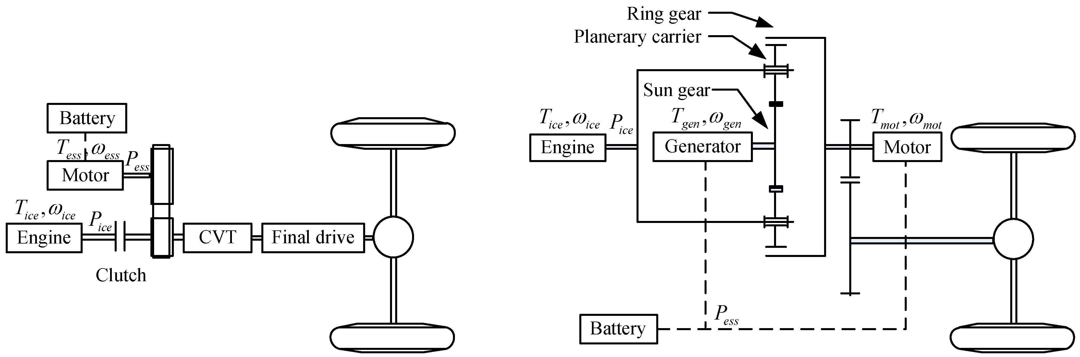
In general, the electromechanical coupling systems of HEVs are classified into three categories: torque coupling, speed coupling, and power coupling systems. The QPIS proposed in this paper is suitable for power-coupling HEVs, whose configurations are depicted in Figure 1, satisfying the assumptions as follows.

Figure 1. Schematic diagrams of HEVs. (a) HEV equipt with a CVT; (b) HEV equipt with a planetary gear mechanism.

Figure 1. Schematic diagrams of HEVs. (a) HEV equipt with a CVT; (b) HEV equipt with a planetary gear mechanism.

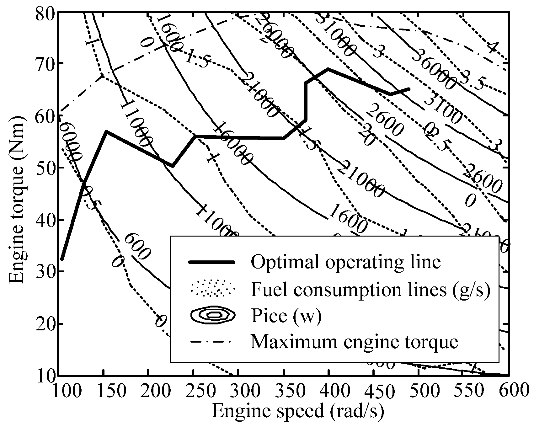
(a) A continuously-variable transmission (CVT) adopted in Figure 1a or a planetary gear mechanism adopted in Figure 1b (such as the Toyota Prius and Ford Escape Hybrid) makes it possible for the engine to always operate on an optimal operating line as the bold solid one plotted in Figure 2. Every engine operating point of optimal operating line is confined to a specific output torque and speed and has the minimum fuel consumption [32]. In other words, for a given engine power $P_{\text{ice}}$, we can determine an optimal engine operating point $\left[T_{\text{ice}}^{\text{*}},{\omega }_{\text{ice}}^{\text{*}}\right]$ based on this optimal operating line. Thus control variables of energy management for HEVs are reduced from the torque and speed to only the power.

(b) Through reasonably choosing battery capacity, the battery SOC mainly varies in a narrow region, for example, 0.6–0.8, so the charge-discharge characteristics of battery are almost invariable. In other words, the open-circuit voltage and equivalent internal resistance of battery can be regarded as constants [32].

Figure 2. Optimal operating line of the engine.

Figure 2. Optimal operating line of the engine.

(c) The motor driving system has sufficient capability of short-time overload (overtorque or overpower), adequate field-weaking range, and wide high-efficiency area. The motor efficiency is not sensitive to engine operating points.

(d) Because the dynamic response time of engine or motor is much shorter than that of vehicle accelerating or decelerating and battery charging or discharging, the dynamic process of engine and motor can be neglected and only static efficiency models need to be considered [22].

In this study, a pedal position is interpreted as a velocity demand $v^{*}$. The proposed algorithm can calculate the engine power $P_{\text{ice}}^{\text{*}}$ and motor power $P_{\text{ess}}^{\text{*}}$ based on current velocity, desired velocity $v^{*}$, current SOC, and desired SOC. For the vehicle in Figure 1a, the optimal operation point $\left[T_{\text{ice}}^{\text{*}},{\omega }_{\text{ice}}^{\text{*}}\right]$ can be determined by $P_{\text{ice}}^{\text{*}}$, then we can jointly regulate the engine throttle and transmission ratio of CVT to make the engine run on the optimal operating line and satisfy $T_{\text{ice}}^{\text{*}}\times {\omega }_{\text{ice}}^{\text{*}}=P_{\text{ice}}^{\text{*}}$. Meanwhile, the motor speed ${\omega }_{\text{ess}}^{\text{*}}$ is determined by the CVT ratio and $P_{\text{ess}}^{\text{*}}=T_{\text{ess}}^{\text{*}}\times {\omega }_{\text{ess}}^{\text{*}}$ can be satisfied by regulating the motor torque $T_{\text{ess}}^{\text{*}}$. For the vehicle in Figure 1b, the ring gear is connected to the final drive, so current vehicle velocity dictates the speed of the motor and ring gear. By jointly regulating the generator speed and engine throttle, the engine can run on the optimal operating line and satisfy $P_{\text{ice}}=P_{\text{ice}}^{\text{*}}$. At the same time, we can regulate the motor torque to ensure the sum of the motor and generator power is equal to $P_{\text{ess}}^{\text{*}}$. In the following, we take the hybrid system in Figure 1a as an example to derive the QPIS. The main parameters of the vehicle originated from ADVISOR are listed in Table 1.

Table 1. Vehicle parameters.

Vehicle unit	Parameter
Engine FC_SI41emis	Displacement: 1.0 L
	Maximum power: 41 kW @ 5700 rpm
	Maximum torque: 81 Nm @ 3477 rpm
Battery ESS_NIMH	Capacity: 6 Ah
	Voltage: 308 V
Motor MC_PRIUS_JPN	Maximum power: 31 kW
Transmission efficiency	0.71–0.93
Rotating mass coefficient	1.1
Frontal area	2.0 m2
Aerodynamic drag coefficient	0.335
Rolling resistance coefficient	0.009
Vehicle total mass	1287 kg

Table 1. Vehicle parameters.

Vehicle unit	Parameter
Engine FC_SI41emis	Displacement: 1.0 L
	Maximum power: 41 kW @ 5700 rpm
	Maximum torque: 81 Nm @ 3477 rpm
Battery ESS_NIMH	Capacity: 6 Ah
	Voltage: 308 V
Motor MC_PRIUS_JPN	Maximum power: 31 kW
Transmission efficiency	0.71–0.93
Rotating mass coefficient	1.1
Frontal area	2.0 m2
Aerodynamic drag coefficient	0.335
Rolling resistance coefficient	0.009
Vehicle total mass	1287 kg

2.1. Nonlinear HEV Model for Simulations

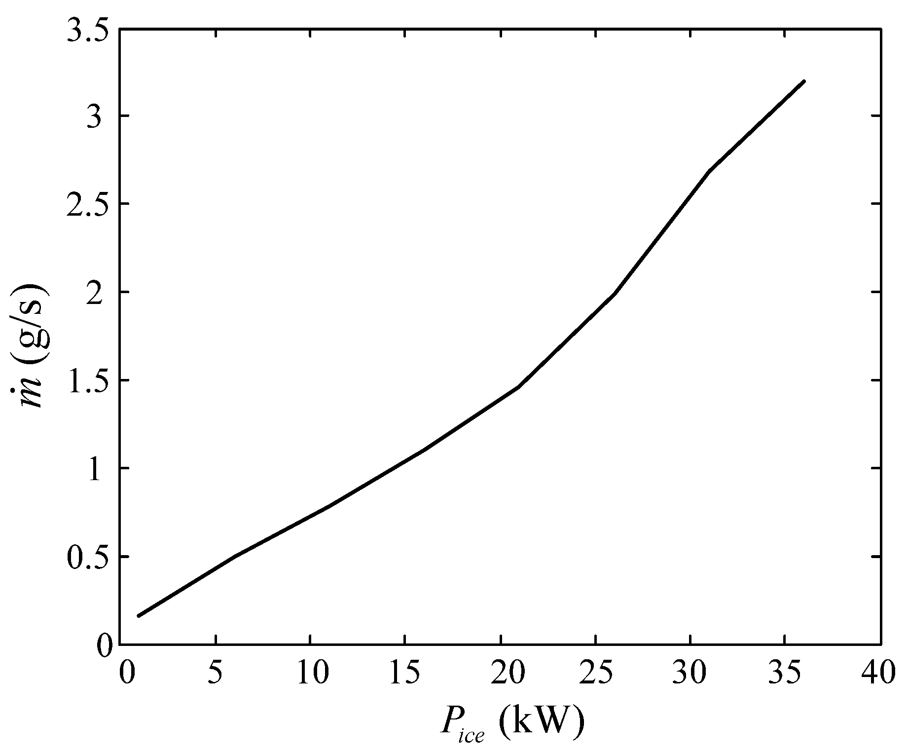
The MAP of Engine FC_SI41emis and its optimal operating line are shown in Figure 2. The corresponding optimal fuel consumption line is plotted in Figure 3, which shows the relation between $P_{\text{ice}}$ and the fuel consumption rate $\dot{m}$. The fuel consumption of control algorithms in simulations is the integral of $\dot{m}$ over the whole driving cycle.

Figure 3. Optimal fuel consumption line.

Figure 3. Optimal fuel consumption line.

If the vehicle is running at the velocity $v$, the driving force $F$ can be calculated by:

$$\delta m\frac{\text{d}v}{\text{d}t}+mg{f}_r\cos \theta +mg\sin \theta +\frac{1}{2}\rho C_D{A}_f{v}^2=F{\eta }_t^p$$

(1)

where $\delta$ is the rotating mass coefficient; $m$ is the vehicle total mass, including the passengers and cargo; $g$ is the gravitational acceleration constant; $f_r$ is the rolling resistance coefficient; $\theta$ is the road slope; $\rho$ is the air density; $C_D$ is the aerodynamic drag coefficient; $A_f$ is the vehicle frontal area, and ${\eta }_t$ is the transmission efficiency, which is the function of vehicle velocity, load torque and CVT ratio, $p=\{\begin{array}{ll}1,& P_{\text{req}}>0\\ -1,& P_{\text{req}}\le 0\end{array}$ and $P_{\text{req}}$ is the requested power, which satisfies:

$$P_{\text{req}}=P_{\text{ice}}+P_{\text{ess}}$$

(2)

where $P_{\text{ice}}$ is the engine power and $P_{\text{ess}}$ is the motor power.

Multiplying Equation (1) by $v$, we will get the vehicle dynamic model:

$$\frac{1}{2}\delta m\frac{\text{d}{v}^2}{\text{d}t}+mg{f}_{r}v\cos \theta +mgv\sin \theta +\frac{1}{2}\rho C_D{A}_f{v}^3=\left(P_{\text{ice}}+P_{\text{ess}}\right){\eta }_t^p$$

(3)

The energy storage system is a 6Ah Ni-MH battery. The battery power $P_{\text{bat}}$ satisfies:

$$\frac{\text{d}\left(E\cdot \text{SOC}\right)}{\text{d}t}=-\frac{V\left(V-\sqrt{V^2-4R{P}_{\text{bat}}}\right)}{2R}$$

(4)

where $E$ is the total energy of battery; $E\cdot \text{SOC}$ is the residual energy of battery; $V$ and $R$ are the open-circuit voltage and equivalent internal resistance, respectively [32].

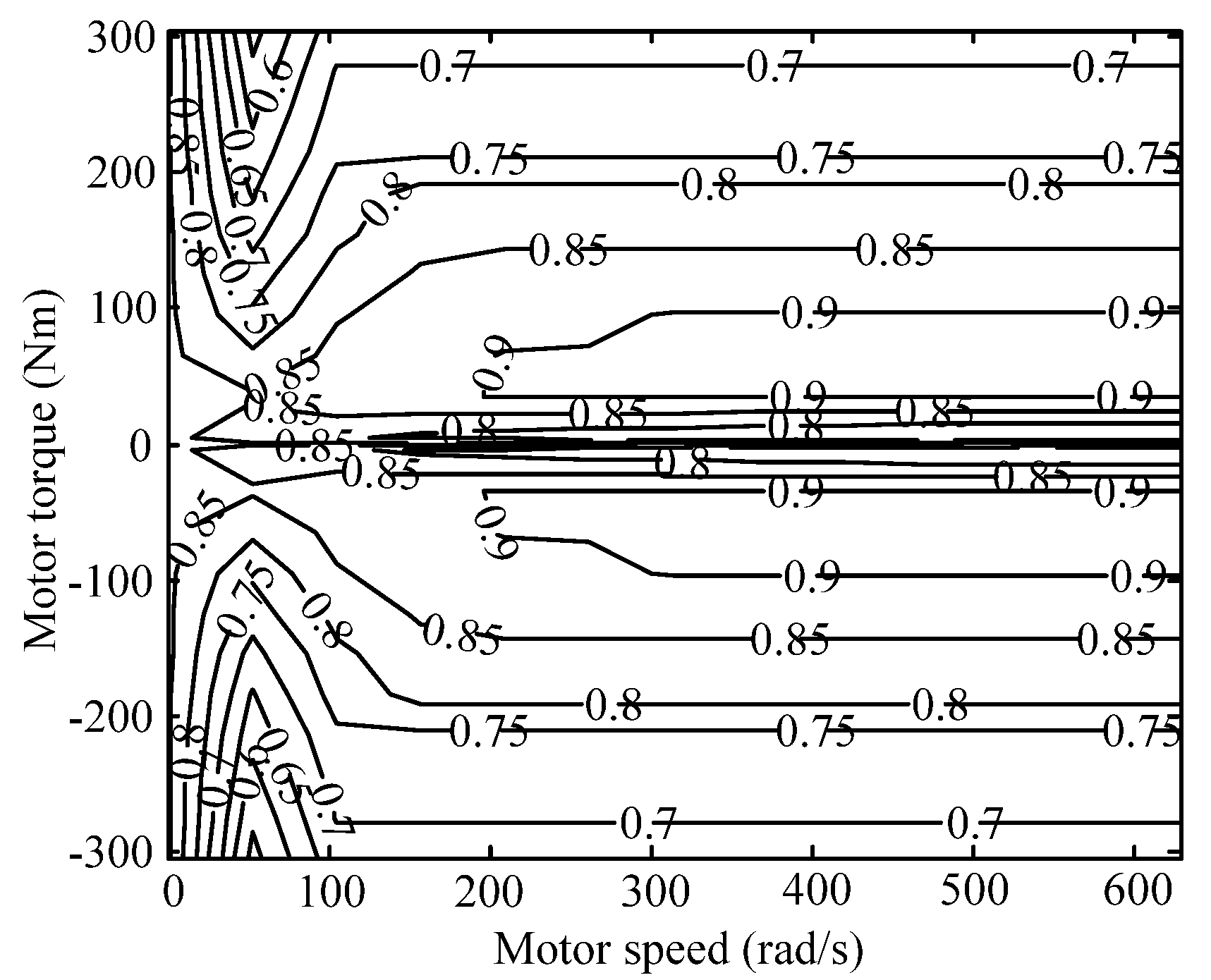
As assumptions stated above, a permanent magnet motor is selected, whose efficiency map is shown in Figure 4. The motor power $P_{\text{ess}}$ can be expressed as:

$$P_{\text{bat}}=P_{\text{ess}}/{\eta }_m^k$$

(5)

where ${\eta }_m$ is the motor efficiency, which is the function of motor torque and motor speed, $k=\{\begin{array}{ll}1,& P_{\text{bat}}>0\\ -1,& P_{bat}\le 0\end{array}$ ($P_{bat}>0$ indicates that the battery is discharging and $P_{\text{bat}}\le 0$ indicates that the battery is charging).

Figure 4. Efficiency map of the motor.

Figure 4. Efficiency map of the motor.

2.2. Linear HEV Model for QPIS

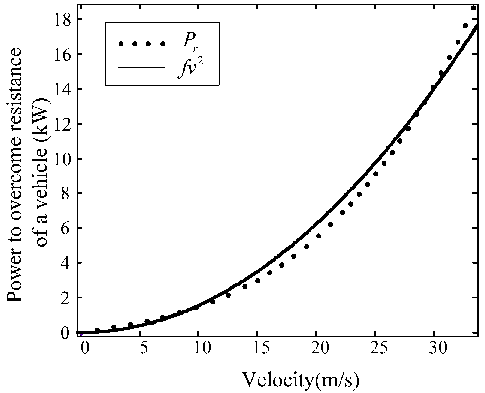
To utilize linear quadratic optimal control theory to derive control functions of QPIS, we should establish a linear model of HEV. The dot line shown in Figure 5 depicts the relationship between $v$ and the power to overcome resistance $P_r=mg{f}_{r}v\cos \theta +mgv\sin \theta +\frac{1}{2}\rho C_D{A}_f{v}^3$, when $\theta =0$. The correlation between $v$ and $P_r$ should be fitted as a parabola, $f{v}^2$ (the solid line, which is available in the involved power range), to obtain the linear model, so we can replace $P_r$ with $f{v}^2$ ($f=15.57$). In addition, ${\eta }_t$ should be replaced by average efficiency, ${\overline{\eta }}_t=0.862$. Then the vehicle dynamic model can be expressed as Equation (6) with $x_1=v^2$ as the state variable:

$$\frac{1}{2}\delta m\frac{\text{d}{v}^2}{\text{d}t}+f{v}^2=\left(P_{\text{ice}}+P_{\text{ess}}\right){\overline{\eta }}_t^p$$

(6)

Figure 5. Relationship between $P_r$ and $f{v}^2$.

Figure 5. Relationship between $P_r$ and $f{v}^2$.

For the battery, when the SOC changes within the interval [0.6,0.8] and $P_{\text{bat}}$ varies in the interval [−15 kW,0], the battery charging efficiency calculated by ${\left(P_{\text{bat}}/\left(V\left(V-\sqrt{V^2-4R{P}_{\text{bat}}}\right)/2R\right)\right)}^{-1}$ ranges in $\left[0.8988,1\right]$. When the SOC changes within the interval [0.6,0.8] and $P_{\text{bat}}$ varies in the interval [0,15 kW], the battery discharging efficiency calculated by $P_{\text{bat}}/\left(V\left(V-\sqrt{V^2-4R{P}_{\text{bat}}}\right)/2R\right)$ ranges in [1,0.7664]. Then the average efficiency of battery can be computed, i.e., ${\overline{\eta }}_{\text{bat}}^k=\{\begin{array}{ll}0.8976,& P_{\text{bat}}>0\\ \frac{1}{0.9459},& P_{\text{bat}}\le 0\end{array}$. For the motor, the efficiency map is symmetric about the horizontal axis as shown in Figure 4, based on which the average efficiency of motor is ${\overline{\eta }}_m=0.8$.

Thus, the linear relation between the state variable $x_2=E\cdot \text{SOC}$ and $P_{\text{ess}}$ is:

$$\frac{\text{d}\left(E\cdot \text{SOC}\right)}{\text{d}t}=-\frac{P_{\text{ess}}}{{\overline{\eta }}_{\text{bat}}^k{\overline{\eta }}_m^k}$$

(7)

In the above linearization process, the linear vehicle dynamic model (6) is obtained when $\theta =0$. However, in fact, vehicles usually run on slopes, which degrades the vehicle drivability and SOC sustainability. To overcome the influences caused by road slopes, two integral actions, $x_3={\displaystyle \int \left({\left(v^{*}\right)}^2-v^2\right)}\text{d}t$ and $x_4={\displaystyle \int E\cdot \left({\text{SOC}}^{*}-\text{SOC}\right)}\text{d}t$, are added to the HEV model as two extended state variables. As known from linear quadratic optimal control theory, the control law is the feedback of system states, so the control variables of QPIS contain not only the feedback of current states ($v$ and $E\cdot \text{SOC}$) but also the integrals of the deviations of actual states from commands ($v^{*}$ and $E\cdot {\text{SOC}}^{\text{*}}$). Such integral actions can eliminate the influences of various driving conditions on the control performance of QPIS, especially overcome the influences of road slopes effectively.

Selecting $\mathit{x}=\left[\begin{array}{c}{x}_1\\ \begin{array}{l}{x}_2\\ x_3\\ x_4\end{array}\end{array}\right]=\left[\begin{array}{c}{v}^2\\ E\cdot \text{SOC}\\ {\displaystyle \int \left({\left(v^{*}\right)}^2-v^2\right)}\text{d}t\\ {\displaystyle \int E\cdot \left({\text{SOC}}^{*}-\text{SOC}\right)}\text{d}t\end{array}\right]$ as state variables and $\mathit{u}=\left[\begin{array}{c}{u}_1\\ u_2\end{array}\right]=\left[\begin{array}{c}{P}_{\text{ice}}\\ P_{\text{ess}}\end{array}\right]$ as control variables, and combining Equations (6) and (7), we can establish the linear HEV system as:

$$\dot{\mathit{x}}=A\mathit{x}+B_u\mathit{u}+B_r{\mathit{z}}^{*}$$

(8)

where $A=\left[\begin{array}{cccc}-\frac{2f}{\delta m}& 0& 0& 0\\ 0& 0& 0& 0\\ -1& 0& 0& 0\\ 0& -1& 0& 0\end{array}\right]$, $B_u=\left[\begin{array}{cc}\frac{2{\overline{\eta }}_t^p}{\delta m}& \frac{2{\overline{\eta }}_t^p}{\delta m}\\ 0& -\frac{1}{{\overline{\eta }}_{\text{bat}}^k{\overline{\eta }}_m^k}\\ 0& 0\\ 0& 0\end{array}\right]$, and $B_r=\left[\begin{array}{cc}0& 0\\ 0& 0\\ 1& 0\\ 0& 1\end{array}\right]$ are the coefficient matrixes of the system; $z^{*}=\left[\begin{array}{c}{x}_1^{*}\\ x_2^{*}\end{array}\right]=\left[\begin{array}{c}{\left(v^{*}\right)}^2\\ E\cdot {\text{SOC}}^{*}\end{array}\right]$ are the commands; $v^{*}$ is the desired vehicle velocity decided by the pedal position, and ${\text{SOC}}^{*}$ is the desired battery SOC (a constant that the SOC changes around to efficiently use and protect the battery). It should be noted that the aim of linearizing the original nonlinear vehicle model is just to utilize linear quadratic optimal control theory to obtain the QPIS. The HEV model to be controlled by the strategies involved in the simulations is the same nonlinear one introduced in Section 2.1.

3. Power Management Strategy Based on Quadratic Performance Index

To compare with the proposed strategy in this paper, PMP is briefly introduced at first. In fact, applying PMP to solve the minimum fuel consumption problem of HEVs is to search for the motor power $P_{\text{ess}}\left(t\right)$ to minimize the fuel consumption under a specific driving cycle. Since the driving cycle is known previously, the requested power $P_{\text{req}}\left(t\right)$ can be calculated based on vehicle parameters when the vehicle is running along the vehicle velocity line of driving cycle. In this way, for the given $P_{\text{req}}\left(t\right)$, which satisfies the Equation (2), the above minimum fuel consumption control problem is to calculate $P_{\text{ess}}\left(t\right)$ to minimize the integral performance index as:

$$J={\displaystyle {\int }_{t_0}^{t_f}\dot{m}\left(P_{\text{ice}}\left(t\right)\right)\text{d}t}$$

(9)

where $\dot{m}\left(P_{\text{ice}}\right)$ is the fuel consumption rate of the engine when its output power is $P_{\text{ice}}$. The relationship between $\dot{m}\left(P_{\text{ice}}\right)$ and $P_{\text{ice}}$ is plotted in Figure 3 based on the assumption (a) in Section 2. Meanwhile, $P_{\text{ess}}\left(t\right)$ satisfies Equations (4) and (5), the terminal constraint condition:

$$\text{SOC}\left(t_f\right)=\text{SOC}\left(t_0\right)$$

(10)

and the maximum and minimum constraints of $P_{\text{ice}}$ and $P_{\text{ess}}$.

According to PMP, the necessary condition that the solution of above optimal control problem should satisfy is to minimize the Hamiltonian:

$$H=\dot{m}\left(P_{\text{req}}-P_{\text{ess}}\right)\text{+}\lambda \cdot \frac{\text{d}\left(E\cdot \text{SOC}\right)}{\text{d}t}=\dot{m}\left(P_{\text{req}}-P_{\text{ess}}\right)-\lambda \cdot \frac{V\left(V-\sqrt{V^2-4R{P}_{\text{ess}}/{\eta }_m^k}\right)}{2R}$$

(11)

for each sampling instant [32]. In Equation (11), $\lambda <0$ is called co-state and satisfies the co-state equation

$$\dot{\lambda }=-\frac{\partial H}{\partial \left(E\cdot \text{SOC}\right)}$$

(12)

Since $\dot{m}$ and $\frac{V\left(V-\sqrt{V^2-4R{P}_{\text{ess}}/{\eta }_m^k}\right)}{2R}$ are not the functions of SOC, (i.e., the assumption (b) in Section 2), $\lambda$ is a constant [32]. Known from the Introduction, $\lambda$ can be interpreted as an equivalent factor to equate the electrical usage of a battery to the virtual fuel consumption. Therefore, an empirical value of equivalent factor can be chosen as the initial co-state. For example, 30 kWh of battery energy corresponds to 10 L gasoline; then we can calculate the empirical value that equals −6.935 × 10⁻⁵ as the initial co-state. For a specific driving cycle and a set co-state, $P_{\text{ess}}\left(t\right)$ can be calculated by minimizing Equation (11) in its feasible range for each sampling instant $t$. If $\text{SOC}\left(t_f\right)$ of the battery controlled by $P_{\text{ess}}\left(t\right)$ satisfies $\left|\text{SOC}\left(t_f\right)-\text{SOC}\left(t_0\right)\right|\le 0.05$, $P_{\text{ess}}\left(t\right)$ is the result that we desire in this paper. If $\text{SOC}\left(t_f\right)-\text{SOC}\left(t_0\right)>0.05$ (or $\text{SOC}\left(t_f\right)-\text{SOC}\left(t_0\right)<-0.05$), a new co-state, whose absolute value is smaller (or greater) than the absolute value of empirical co-state, is chosen to repeat the above calculation process. Obviously, to achieve optimal fuel economy, $\lambda$ are different for different driving cycles. Moreover, $\dot{m}$ and $\frac{\text{d}\left(E\cdot \text{SOC}\right)}{\text{d}t}$ in Equation (11) are both nonlinear; thus, it is a relatively large calculation to minimize the Equation (11) in the feasible range of $P_{\text{ess}}\left(t\right)$ for each sampling instant $t$. In the following, an EMS is obtained based on the quadratic performance index to overcome the disadvantages of PMP with little loss in fuel economy.

3.1. Power-Split Strategy Based on Quadratic Performance Index

For the system (8), we try to find a linear state feedback control $\mathit{u}=L\mathit{x}$ to ensure the system stability. If ${\mathit{z}}^{*}=\left[\begin{array}{c}{x}_1^{*}\\ x_2^{*}\end{array}\right]=\left[\begin{array}{c}{\left(v^{*}\right)}^2\\ E\cdot {\text{SOC}}^{*}\end{array}\right]$ is set to be constant, after the dynamic regulation process is completed, the vehicle velocity is $\sqrt{x_1}=v^{\ast }$, the battery residual energy is $x_2=E\cdot {\text{SOC}}^{*}$, the engine power is $u_1=f{\left(v^{\ast }\right)}^2/{\eta }_t^p$, the motor power is $u_2=0$, and the corresponding outputs of the integral regulator, $x_3$ and $x_4$, are constant and satisfies ${\mathit{u}}_{ss}=L{\mathit{x}}_{ss}$. We define these steady states and control inputs as ${\mathit{x}}_{ss}$ and ${\mathit{u}}_{ss}$, the deviation of actual states from steady ones as $\tilde{\mathit{x}}=\mathit{x}-{\mathit{x}}_{ss}$, and the deviation of actual control inputs from steady ones as $\tilde{\mathit{u}}=\mathit{u}-{\mathit{u}}_{ss}$. Since $t\to \infty$, $\tilde{\mathit{x}}\to 0$, and $\tilde{\mathit{u}}\to 0$, the performance index about $\tilde{\mathit{x}}$ and $\tilde{\mathit{u}}$:

$$\tilde{J}=\frac{1}{2}{\displaystyle {\int }_{t_0}^{t_f}\left[{\tilde{\mathit{x}}}^{\text{T}}Q\tilde{\mathit{x}}+{\tilde{\mathit{u}}}^{\text{T}}R\tilde{\mathit{u}}\right]\text{d}t}$$

(13)

should be finite, and the solution to minimize the above quadratic performance index can be obtained based on the regulator theory of optimal control theory. The control law has the form of state feedback as:

$$\tilde{\mathit{u}}=L\left(t\right)\tilde{\mathit{x}}=-R^{-1}{B}_u^{\text{T}}K\left(t\right)\tilde{\mathit{x}}$$

(14)

where $K\left(t\right)=K{\left(t\right)}^{\text{T}}$ is the solution of differential Riccati equation; and $L\left(t\right)=-R^{-1}{B}_u^{\text{T}}K\left(t\right)$ is the state feedback matrix. Known from the quadratic optimal control theory, if $t_f$ is large enough, $K\left(t\right)$ convergences to its terminal value only when $t$ approaches $t_f$, and in the most time of $\left[t_0,t_f\right]$, $K\left(t\right)$ is constant and satisfies the algebraic Riccati equation:

$$KA+A^{T}K-K{B}_u{R}^{-1}{B}_u^{\text{T}}K+Q=0$$

(15)

In this way, $\tilde{\mathit{u}}=L\tilde{\mathit{x}}$ and ${\mathit{u}}_{ss}=L{\mathit{x}}_{ss}$, where $L=-R^{-1}{B}_u^{\text{T}}K$, the control variable to minimize $\tilde{J}$ is a form of state feedback:

$$\mathit{u}=\tilde{\mathit{u}}+{\mathit{u}}_{ss}=L\tilde{\mathit{x}}+L{\mathit{x}}_{ss}=L\mathit{x}$$

(16)

Additionally, the system stability can be ensured because $A+B_{u}L$ is a stable matrix based on linear quadratic optimal control theory.

For the system (8), the changes of $B_u$ in value caused by the energy flow direction (indicated by $p$ and $k$) lead to the variation of $K$. For the simplification of this algorithm, $B_u$ is rewritten as the product of two matrices:

$$B_u=\left[\begin{array}{cc}\frac{2{\overline{\eta }}_t^p}{\delta m}& \frac{2{\overline{\eta }}_t^p}{\delta m}\\ 0& -\frac{1}{{\overline{\eta }}_{\text{bat}}^k{\overline{\eta }}_m^k}\\ 0& 0\\ 0& 0\end{array}\right]=\left[\begin{array}{cc}\frac{2}{\delta m}& \frac{2}{\delta m}\\ 0& -1\\ 0& 0\\ 0& 0\end{array}\right]\left[\begin{array}{cc}{\overline{\eta }}_t^p& {\overline{\eta }}_t^p-\frac{1}{{\overline{\eta }}_{\text{bat}}^k{\overline{\eta }}_m^k}\\ 0& \frac{1}{{\overline{\eta }}_{\text{bat}}^k{\overline{\eta }}_m^k}\end{array}\right]$$

(17)

Setting ${B^{\prime }}_u=\left[\begin{array}{cc}\frac{2}{\delta m}& \frac{2}{\delta m}\\ 0& -1\\ 0& 0\\ 0& 0\end{array}\right]$, $\text{η}=\left[\begin{array}{cc}{\overline{\eta }}_t^p& {\overline{\eta }}_t^p-\frac{1}{{\overline{\eta }}_{\text{bat}}^k{\overline{\eta }}_m^k}\\ 0& \frac{1}{{\overline{\eta }}_{\text{bat}}^k{\overline{\eta }}_m^k}\end{array}\right]$ and ${\mathit{u}}^{\prime }=\text{η}\mathit{u}$ is the engine and motor power excluding the loss power of transmission, motor, and battery, the system (8) can be rewritten as:

$$\dot{\mathit{x}}=A\mathit{x}+{B^{\prime }}_u{\mathit{u}}^{\prime }+B_r{\mathit{z}}^{*}$$

(18)

where ${B^{\prime }}_u$ is constant so that the variation of $K$ caused by $B_u$ can be avoided.

Accordingly, the performance index is rewritten as:

$$\tilde{J}=\frac{1}{2}{\displaystyle {\int }_{t_0}^{t_f}\left[{\tilde{\mathit{x}}}^{\text{T}}Q\tilde{\mathit{x}}+{{\tilde{\mathit{u}}}^{\prime }}^{\text{T}}{R}^{\prime }{\tilde{\mathit{u}}}^{\prime }\right]dt}$$

(19)

where $Q=\left[\begin{array}{cccc}{\gamma }_1& 0& 0& 0\\ 0& {\gamma }_2& 0& 0\\ 0& 0& {\gamma }_3& 0\\ 0& 0& 0& {\gamma }_4\end{array}\right]\ge 0$ and $R^{\prime }=\left[\begin{array}{cc}{\gamma }_5& 0\\ 0& {\gamma }_6\end{array}\right]>0$ are the matrixes of weight coefficients. We can quicken the regulating process of state and control variables by increasing the corresponding weight coefficient of the deviation term in $\tilde{J}$. The calibration of weight coefficients needs to ensure vehicle drivability, prevent large fluctuations of SOC, cut peaks and fill valleys of engine power, and smooth the engine power to indirectly reduce fuel consumption.

For the optimal control problem of the system (18) and performance index (19), the solution has the form of Equation (16):

$${\mathit{u}}^{\prime }=L^{\prime }\mathit{x}$$

(20)

where $L^{\prime }=-{R^{\prime }}^{-1}{B^{\prime }}_u^{\text{T}}{K}^{\prime }$ is the matrix of state feedback and $K^{\prime }$ satisfies:

$$K^{\prime }A+A^T{K}^{\prime }-K^{\prime }{B^{\prime }}_u{R^{\prime }}^{-1}{B^{\prime }}_u^{\text{T}}{K}^{\prime }+Q=0$$

(21)

Then, the engine power and motor power can be calculated by:

$$\mathit{u}={\text{η}}^{-1}{\mathit{u}}^{\prime }=-{\text{η}}^{-1}{R^{\prime }}^{-1}{B^{\prime }}_u^{\text{T}}{K}^{\prime }\mathit{x}$$

(22)

where $\text{η}=\left[\begin{array}{cc}{\overline{\eta }}_t^p& {\overline{\eta }}_t^p-\frac{1}{{\overline{\eta }}_{\text{bat}}^k{\overline{\eta }}_m^k}\\ 0& \frac{1}{{\overline{\eta }}_{\text{bat}}^k{\overline{\eta }}_m^k}\end{array}\right]$ changes with $p$ and $k$, based on $P_{\text{req}}$ and $P_{\text{bat}}$, respectively, i.e., $p=\{\begin{array}{ll}1,& P_{\text{req}}>0\\ -1,& P_{\text{req}}\le 0\end{array}$ and $k=\{\begin{array}{ll}1,& P_{\text{bat}}>0\\ -1,& P_{\text{bat}}\le 0\end{array}$.

3.2. Two Control Modes

To further improve the fuel economy, two rules are designed to switch control modes (electric mode and hybrid mode) based on $P_{\text{req}}$ for avoiding inefficient engine operation. The selection of a switch point between the two control modes is combined with engine characteristics, vehicle parameters, and the principle of benefiting fuel economy. In this paper, the switch point is $P_{\text{req}}=P_0$, which is decided by comparing the energy conversion efficiency of a vehicle propelled separately by an engine and a motor. That is, when $P_{\text{req}}=P_0$, the efficiency of vehicle propelled solely by an engine is equal to the product of the efficiency of a vehicle propelled solely by a motor and the efficiency of the battery charged by an engine [38]. The two control modes are realized by choosing different weight coefficients of the quadratic performance index as follows:

(1) If $P_{\text{req}}\le P_0$: the battery should provide the total driving power to avoid inefficient engine operation or recover the braking energy that will be stored in the battery. Thus, we should set ${\gamma }_5\to \infty$ to make $P_{\text{ice}}$ approach to zero, and ${\gamma }_2=0$, ${\gamma }_4=0$ to temporarily not consider the constraint of SOC unless SOC reaches the maximum or minimum value.

(2) If $P_{\text{req}}>P_0$: the engine and battery should provide requested power together. The battery shares the driving energy to restrain fluctuations of $P_{\text{ice}}$. Now the constraint of SOC should be necessarily involved in the performance index for battery energy sustainability.

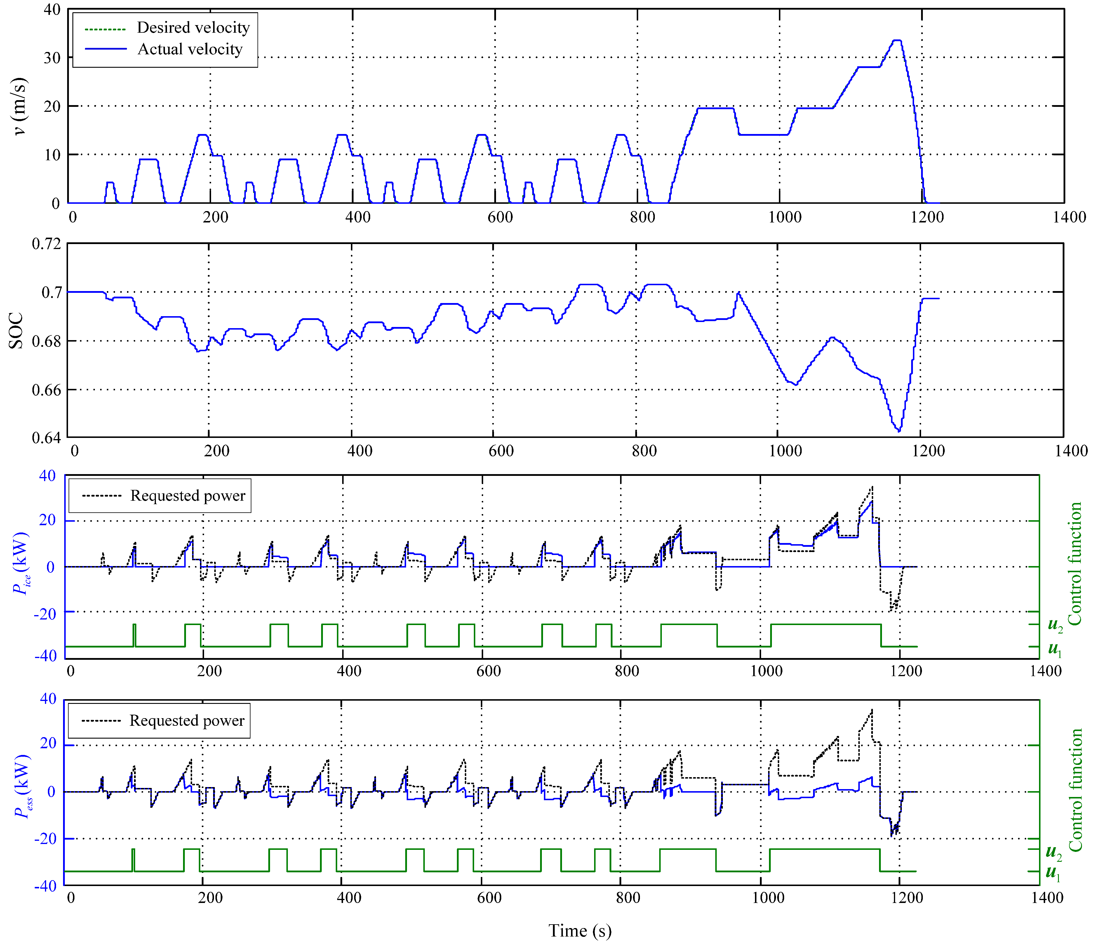
In general, the weight coefficients of two control modes can be calibrated by a test, where the desired SOC is 0.7 and the desired vehicle velocity line is shown in Figure 6. In the calibration, to tune the weight coefficients of $Q$ is similar to design a proportional integral (PI) controller: ${\gamma }_1$ and ${\gamma }_2$ correspond to proportional gains, ${\gamma }_3$ and ${\gamma }_4$ correspond to integral gains. In other words, increasing ${\gamma }_1$ and ${\gamma }_3$ results in faster response and smaller tracking errors of $v$, but paying the price of larger fluctuations of SOC and more power provided by the engine and motor that may exceed their feasible bounds. Similarly, increasing ${\gamma }_2$ and ${\gamma }_4$ quickens the response of SOC and maintains SOC nearer to 0.7 with a little influence on trajectories of $v$, $P_{\text{ice}}$ and $P_{\text{ess}}$, but weakens the buffering effect of the battery. Additionally, the fluctuations ranges of $P_{\text{ice}}$ (or $P_{\text{ess}}$) can be restricted within the feasible bounds by appropriately increasing ${\gamma }_5$ (or ${\gamma }_6$) with a slight increment of tracking errors of $v$. According to the above changing laws about the control effect over weight coefficients, we can tune the weight coefficients of two control modes by compromising between the tracking errors of states and fluctuation ranges of control variables until obtaining a relatively better result of vehicle velocity error, final SOC, and fuel economy. In this paper, the calibrated weight coefficients and corresponding $K^{\prime }$ and $L^{\prime }$ are given in Table 2. The test results with above weight coefficients are shown in Figure 6.

Table 2. Weight coefficients and state feedback matrixes of two rules.

Operational condition	Weight coefficients	K′	L′
$P_{req}\le P_0$	$\begin{array}{l}{Q}_1=\left[\begin{array}{cccc}{10}^9& 0& 0& 0\\ 0& 0& 0& 0\\ 0& 0& 4\times {10}^{10}& 0\\ 0& 0& 0& 0\end{array}\right]\\ {R^{\prime }}_1=\left[\begin{array}{cc}{10}^{20}& 0\\ 0& 40\end{array}\right]\end{array}$	${K^{\prime }}_1=\left[\begin{array}{cccc}2.36\times {10}^8& 0& -8.95\times {10}^8& 0\\ 0& 0& 0& 0\\ -8.95\times {10}^8& 0& 1.06\times {10}^{10}& 0\\ 0& 0& 0& 0\end{array}\right]$	${L^{\prime }}_1=\left[\begin{array}{cccc}0& 0& 0& 0\\ -8337.19& 0& 3.16\times {10}^4& 0\end{array}\right]$
$P_{req}>P_0$	$\begin{array}{l}{Q}_2=\left[\begin{array}{cccc}{10}^9& 0& 0& 0\\ 0& {10}^{-8}& 0& 0\\ 0& 0& 4\times {10}^{10}& 0\\ 0& 0& 0& 5\times {10}^{-7}\end{array}\right]\\ {R^{\prime }}_2=\left[\begin{array}{cc}80& 0\\ 0& 80\end{array}\right]\end{array}$	${K^{\prime }}_2=\left[\begin{array}{cccc}2.36\times {10}^8& 598.77& -8.95\times {10}^8& -3.17\\ 598.77& 1.69& -16.32& -0.0089\\ -8.95\times {10}^8& -16.32& 1.06\times {10}^{10}& 0.10\\ -3.17& -0.0089& 0.10& 9\times {10}^{-5}\end{array}\right]$	${L^{\prime }}_2=\left[\begin{array}{cccc}-4172.34& -0.01& 1.58\times {10}^4& 5.59\times {10}^{-5}\\ -4164.85& 0.01& 1.58\times {10}^4& -5.59\times {10}^{-5}\end{array}\right]$

Table 2. Weight coefficients and state feedback matrixes of two rules.

Operational condition	Weight coefficients	K′	L′
$P_{req}\le P_0$	$\begin{array}{l}{Q}_1=\left[\begin{array}{cccc}{10}^9& 0& 0& 0\\ 0& 0& 0& 0\\ 0& 0& 4\times {10}^{10}& 0\\ 0& 0& 0& 0\end{array}\right]\\ {R^{\prime }}_1=\left[\begin{array}{cc}{10}^{20}& 0\\ 0& 40\end{array}\right]\end{array}$	${K^{\prime }}_1=\left[\begin{array}{cccc}2.36\times {10}^8& 0& -8.95\times {10}^8& 0\\ 0& 0& 0& 0\\ -8.95\times {10}^8& 0& 1.06\times {10}^{10}& 0\\ 0& 0& 0& 0\end{array}\right]$	${L^{\prime }}_1=\left[\begin{array}{cccc}0& 0& 0& 0\\ -8337.19& 0& 3.16\times {10}^4& 0\end{array}\right]$
$P_{req}>P_0$	$\begin{array}{l}{Q}_2=\left[\begin{array}{cccc}{10}^9& 0& 0& 0\\ 0& {10}^{-8}& 0& 0\\ 0& 0& 4\times {10}^{10}& 0\\ 0& 0& 0& 5\times {10}^{-7}\end{array}\right]\\ {R^{\prime }}_2=\left[\begin{array}{cc}80& 0\\ 0& 80\end{array}\right]\end{array}$	${K^{\prime }}_2=\left[\begin{array}{cccc}2.36\times {10}^8& 598.77& -8.95\times {10}^8& -3.17\\ 598.77& 1.69& -16.32& -0.0089\\ -8.95\times {10}^8& -16.32& 1.06\times {10}^{10}& 0.10\\ -3.17& -0.0089& 0.10& 9\times {10}^{-5}\end{array}\right]$	${L^{\prime }}_2=\left[\begin{array}{cccc}-4172.34& -0.01& 1.58\times {10}^4& 5.59\times {10}^{-5}\\ -4164.85& 0.01& 1.58\times {10}^4& -5.59\times {10}^{-5}\end{array}\right]$

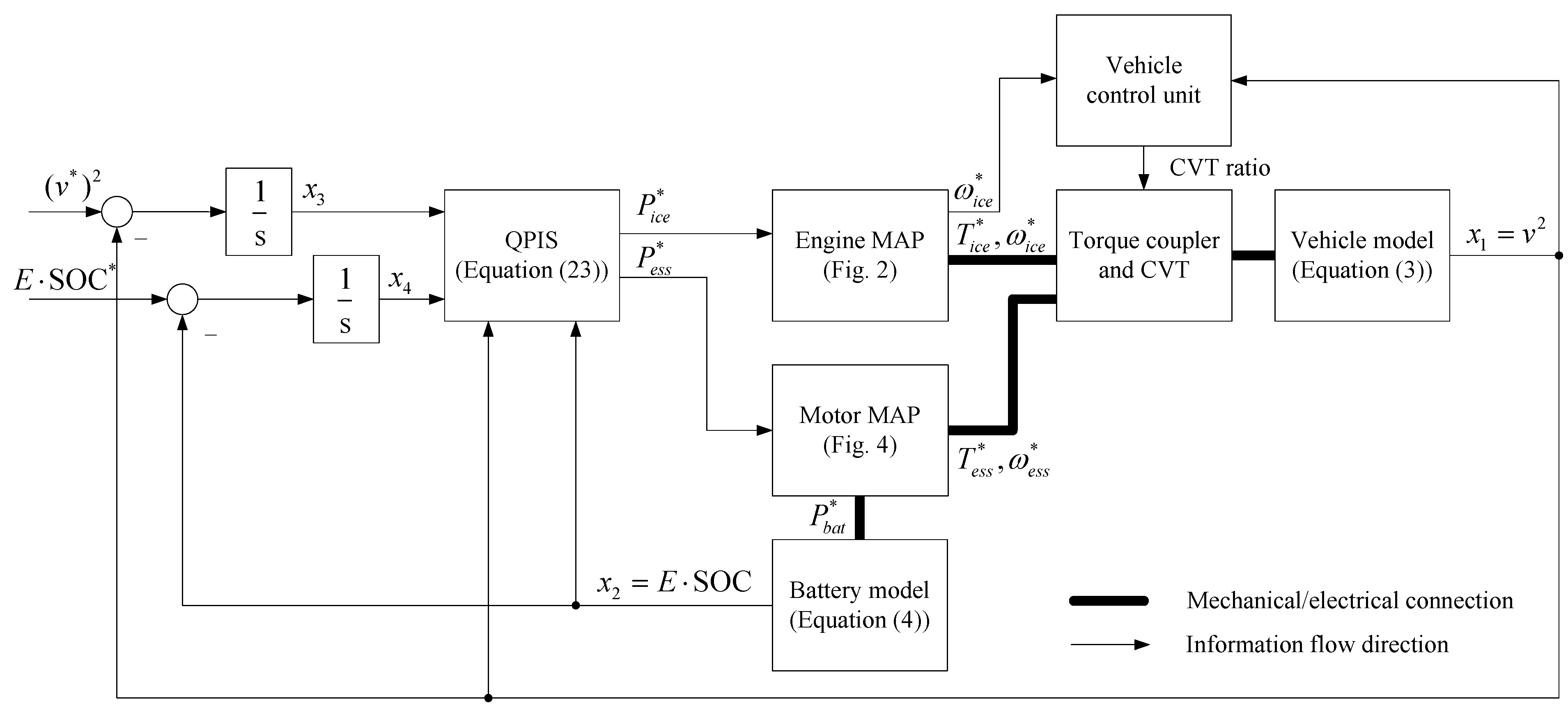
Actually, the more the detailed operational conditions are divided, the better the control effect of QPIS is obtained, but much more complex algorithms are needed, which will weaken the adaptability of QPIS. Eventually, the concrete form of QPIS is:

$$\{\begin{array}{ll}{\mathit{u}}_1=-{\text{η}}^{-1}{R^{\prime }}_1^{-1}{B^{\prime }}_u^{\text{T}}{K^{\prime }}_1\mathit{x},& P_{\text{req}}\le P_0\\ {\mathit{u}}_2=-{\text{η}}^{-1}{R^{\prime }}_2^{-1}{B^{\prime }}_u^{\text{T}}{K^{\prime }}_2\mathit{x},& P_{\text{req}}>P_0\end{array}$$

(23)

The control system of QPIS is shown in Figure 7. It can be observed that the control variables of QPIS are simple linear functions of current system states $\mathit{x}$ without future driving conditions. This interesting feature makes QPIS simply structured and particularly suitable for real-time optimization control. Furthermore, ${\mathit{u}}_1$, and ${\mathit{u}}_2$ are switched based on $P_{\text{req}}$, which is the sum of $P_{\text{ice}}$ and $P_{\text{ess}}$ calculated by QPIS. To avoid frequent switches of control functions at switch points, we necessarily add a hysteresis loop when $P_{\text{req}}=P_0$, of which the switch on and off points are $P_{on}=8\text{\hspace{0.17em}kW}$ and $P_{off}=2\text{\hspace{0.17em}kW}$, respectively, and the engine power and motor power of ${\mathit{u}}_1$ and ${\mathit{u}}_2$ are limited in their respective feasible ranges.

Figure 6. Test results of calibrated weight coefficients.

Figure 6. Test results of calibrated weight coefficients.

Figure 7. Control system diagram of QPIS.

Figure 7. Control system diagram of QPIS.

4. Simulation Results and Discussion

To verify the control performance of proposed QPIS, simulations under different driving cycles, road slopes, and vehicle total masses are conducted in ADVISOR, where the units are redesigned to make ADVISOR, which is a simulator combined with forward and backward approaches, suitable for forward simulation.

4.1. Various Driving Cycle

During the simulations, the weight coefficients of QPIS are the same ones given in Table 2. The initial and desired SOC are set to 0.7. Figure 8 depicts the trajectories of vehicle velocity, battery SOC, engine power and motor power obtained from QPIS under the NEDC cycle. It is found that the desired velocity trajectory is properly tracked with a small average error (0.064 m/s). The SOC trajectory stays near 0.7 with the deviation within 0.06. When $P_{\text{req}}$ is increasing, but less than $P_{\text{on}}$, the control function is ${\mathit{u}}_1$. If $P_{\text{req}}$ continues to increase and becomes greater than $P_{\text{on}}$, the control function is switched to ${\mathit{u}}_2$. In reverse, if $P_{\text{req}}$ decreases, the points to switch control functions are $P_{\text{off}}$. Throughout the driving cycle, the average value of $P_{\text{ess}}$ is about zero and the battery as an energy buffer effectively recycles the braking energy and restrains large fluctuations of $P_{\text{ice}}$.

To confirm that QPIS is independent of driving cycles, more simulations are performed under five other driving cycles. The simulation results of QPIS over six driving cycles, compared with the conventional vehicles, the default energy management strategy (DEMS) in ADVISOR and PMP are summarized in Table 3, where FC_cv is the fuel consumption of conventional cars. It is observed that $\text{SOC}\left(t_f\right)$ of DEMS and QPIS are unequal to $\text{SOC}\left(t_0\right)$. To compare the DEMS and QPIS with PMP, the deviation of $\text{SOC}\left(t_f\right)$ from $\text{SOC}\left(t_0\right)$ is converted to virtual fuel consumption by an equivalent factor $s$, which can be calculated by:

$$s=\frac{E}{D_f{Q}_f{\overline{\eta }}_e{\overline{\eta }}_m{\overline{\eta }}_{cd}}$$

(24)

where $E$ is the total energy of battery; $D_f$ is the fuel density; $Q_f$ is the low heating value; ${\overline{\eta }}_e$ is the average efficiency of engine used to charge the battery; ${\overline{\eta }}_m$ is the average efficiency of motor; and ${\overline{\eta }}_{cd}$ is the average of the battery charging and discharging efficiency. The results of fuel consumption (FC) in Table 3 contain the converted fuel consumption. The DEMS, which is the electric assistant control strategy based on predefined rules in ADVISOR, determines the control mode (including motor regenerating, motor only, engine only, and hybrid mode) based on predefined threshold values, as well as actual states and driving commands. It is suitable for real-time control, but with limited fuel economy.

Figure 8. Simulation results of QPIS over NEDC cycle in ADVISOR.

Figure 8. Simulation results of QPIS over NEDC cycle in ADVISOR.

Table 3. Simulation results of DEMS, PMP, and QPIS over various driving cycles in ADVISOR.

Driving cycle	FCcv (L/100 km)	DEMS		PMP			QPIS
		FC (L/100 km)	SOC (tf)	FC (L/100 km)	SOC (tf)	λ(g/J)	FC (L/100 km)	SOC (tf)
CSHVR	6.9956	5.1110	0.6421	3.4589	0.6989	−6.5929 × 10−5	3.6588	0.7017
UDDS	6.2529	5.2505	0.6423	3.8370	0.6935	−6.4840 × 10−5	3.8616	0.7184
WVUINTER	4.9847	4.5921	0.6633	3.9466	0.6844	−7.0056× 10−5	4.1855	0.6905
FTP	6.1682	5.1168	0.6601	3.8318	0.6998	−6.4466 × 10−5	3.9549	0.6853
NEDC	6.3946	5.3694	0.6667	4.0313	0.6867	−6.8726 × 10−5	4.1185	0.6975
INDIA_URBAN	6.5888	5.2862	0.6401	3.4747	0.6950	−6.7667 × 10−5	3.5842	0.7220

Table 3. Simulation results of DEMS, PMP, and QPIS over various driving cycles in ADVISOR.

Driving cycle	FCcv (L/100 km)	DEMS		PMP			QPIS
		FC (L/100 km)	SOC (tf)	FC (L/100 km)	SOC (tf)	λ(g/J)	FC (L/100 km)	SOC (tf)
CSHVR	6.9956	5.1110	0.6421	3.4589	0.6989	−6.5929 × 10−5	3.6588	0.7017
UDDS	6.2529	5.2505	0.6423	3.8370	0.6935	−6.4840 × 10−5	3.8616	0.7184
WVUINTER	4.9847	4.5921	0.6633	3.9466	0.6844	−7.0056× 10−5	4.1855	0.6905
FTP	6.1682	5.1168	0.6601	3.8318	0.6998	−6.4466 × 10−5	3.9549	0.6853
NEDC	6.3946	5.3694	0.6667	4.0313	0.6867	−6.8726 × 10−5	4.1185	0.6975
INDIA_URBAN	6.5888	5.2862	0.6401	3.4747	0.6950	−6.7667 × 10−5	3.5842	0.7220

It is amazingly found in Table 3 that even if driving cycles are changed, the control effect of QPIS with the same group of weight coefficients remains as excellent as the results under NEDC. Compared to conventional cars, the three EMSes significantly reduce the fuel consumption. Especially, the QPIS and PMP achieve higher fuel economy than DEMS. More importantly, the fuel consumption improvement of QPIS over six driving cycles is quite close (just slightly lower, i.e., less than 4.8% at worst and 0.4% at best) to that of PMP. It is demonstrated that QPIS, which inherits the advantages of real-time performance of DEMS and the improvement in fuel economy of PMP, can be applied to the power assignment for HEVs even if the future driving cycle is unknown.

4.2. Various Road Slopes and Vehicle Total Masses

The influences of $\theta$ and $m$ on the control effect of QPIS are involved in this section because vehicles usually run on slopes and the vehicle total mass may change in practice. In ADVISOR, $\theta$ can be easily added to a driving cycle as a function of distance and $m$ can be easily changed by setting the vehicle parameter. Table 4 and Table 5 show the results of DEMS, QPIS, and PMP when the HEV runs on UDDS cycle with different $\theta$ and $m$, respectively. It is found that the battery SOC is maintained around 0.7 with a little difference of the final value less than 0.06. The fuel economy of QPIS and PMP are still close and much higher than that of DEMS. It is indicated that the QPIS have good adaptability to road slopes and vehicle total masses.

Table 4. Simulation results of PMP and QPIS under UDDS cycle added different road slopes with the driving distance from 0 to 500 m.

tanθ (%)	FCcv (L/100 km)	DEMS		PMP			QPIS
		FC (L/100 km)	SOC (tf)	FC (L/100 km)	SOC (tf)	λ (g/J)	FC (L/100 km)	SOC (tf)
0	6.2529	5.2505	0.6423	3.8370	0.6935	−6.4840 × 10−5	3.8616	0.7184
5	6.4773	5.4736	0.6458	4.0754	0.7058	−6.5332 × 10−5	4.1784	0.7176
10	6.8242	5.7475	0.6473	4.3187	0.7096	−6.5816 × 10−5	4.4947	0.7108

Table 4. Simulation results of PMP and QPIS under UDDS cycle added different road slopes with the driving distance from 0 to 500 m.

tanθ (%)	FCcv (L/100 km)	DEMS		PMP			QPIS
		FC (L/100 km)	SOC (tf)	FC (L/100 km)	SOC (tf)	λ (g/J)	FC (L/100 km)	SOC (tf)
0	6.2529	5.2505	0.6423	3.8370	0.6935	−6.4840 × 10−5	3.8616	0.7184
5	6.4773	5.4736	0.6458	4.0754	0.7058	−6.5332 × 10−5	4.1784	0.7176
10	6.8242	5.7475	0.6473	4.3187	0.7096	−6.5816 × 10−5	4.4947	0.7108

Table 5. Simulation results of PMP and QPIS under UDDS cycle with different vehicle total mass.

m (kg)	FCcv (L/100 km)	DEMS		PMP			QPIS
		FC (L/100 km)	SOC (tf)	FC (L/100 km)	SOC (tf)	λ (g/J)	FC (L/100 km)	SOC (tf)
1287	6.2529	5.2505	0.6423	3.8370	0.6935	−6.4840 × 10−5	3.8616	0.7184
1487	6.7623	5.7164	0.6485	4.1197	0.7006	−6.3367 × 10−5	4.1955	0.7049
1687	7.3431	6.1806	0.6528	4.4033	0.7151	−6.2239 × 10−5	4.5818	0.7061

Table 5. Simulation results of PMP and QPIS under UDDS cycle with different vehicle total mass.

m (kg)	FCcv (L/100 km)	DEMS		PMP			QPIS
		FC (L/100 km)	SOC (tf)	FC (L/100 km)	SOC (tf)	λ (g/J)	FC (L/100 km)	SOC (tf)
1287	6.2529	5.2505	0.6423	3.8370	0.6935	−6.4840 × 10−5	3.8616	0.7184
1487	6.7623	5.7164	0.6485	4.1197	0.7006	−6.3367 × 10−5	4.1955	0.7049
1687	7.3431	6.1806	0.6528	4.4033	0.7151	−6.2239 × 10−5	4.5818	0.7061

5. Conclusions

Hybrid electric vehicles can effectively reduce fuel consumption because they adopt an engine and motor to propel the vehicle together and cancel the engine idling. However, the fuel-saving performance is directly related to EMSes. In theory, the optimal control must look ahead into the future and back into the past. Therefore, the theory-based strategy of HEVs can only achieve sub-optimal control under the condition that the future driving cycle is unknown. As stated in the Introduction, many efforts have been made to solve this problem, such as recognizing driving cycles, predicting driving conditions, and collecting information of future driving conditions by a transportation information system. However, such methods have complex algorithms or a high cost. In this paper, we consider the energy management problem of HEVs from a new perspective and propose a power-split strategy based on a quadratic performance index by approximations in theory. The proposed strategy has a negligible amount of calculation and does not depend on future driving cycles; especially, its fuel economy is very close to the PMP-based optimal control. Simulation results over six driving cycles in ADVISOR validate the above advantages of the proposed strategy, which is worth deeper research.