Echo State Network with Bayesian Regularization for Forecasting Short-Term Power Production of Small Hydropower Plants

Abstract

As a novel recurrent neural network (RNN), an echo state network (ESN) that utilizes a reservoir with many randomly connected internal units and only trains the readout, avoids increased complexity of training procedures faced by traditional RNN. The ESN can cope with complex nonlinear systems because of its dynamical properties and has been applied in hydrological forecasting and load forecasting. Due to the linear regression algorithm usually adopted by generic ESN to train the output weights, an ill-conditioned solution might occur, degrading the generalization ability of the ESN. In this study, the ESN with Bayesian regularization (BESN) is proposed for short-term power production forecasting of small hydropower (SHP) plants. According to the Bayesian theory, the weights distribution in space is considered and the optimal output weights are obtained by maximizing the posterior probabilistic distribution. The evidence procedure is employed to gain optimal hyperparameters for the BESN model. The recorded data obtained from the SHP plants in two different counties, located in Yunnan Province, China, are utilized to validate the proposed model. For comparison, the feed-forward neural networks with Levenberg-Marquardt algorithm (LM-FNN) and the generic ESN are also employed. The results indicate that BESN outperforms both LM-FNN and ESN.

1. Introduction

Small hydropower (SHP) is officially defined as a hydropower plant with installed capacity not greater than 50 MW in China, higher than most countries in the world [1,2]. China has extremely rich SHP resources, which are widely distributed over more than 1700 mountainous counties. SHP plays an important role in China’s rural electricity supply, because approximately half of the territories, one third of the country’s and a quarter of the total population, are dependent upon SHP for rural electricity supply. Nowadays, SHP is the fourth largest power supply behind thermal power, large and medium-sized hydropower and wind power.

In recent decades, a large number of SHP plants in southwest China, where there are rich hydropower resources, have been quickly developed and constructed, in order to meet local power demands, promote local economic development and improve their living conditions. Due to a lack of unified planning, SHP plants have been in disordered development and management for a long time. The power production of SHP plants are ruleless, so that they, to some extent, influence safe and stable operation of the power grid. Therefore, it is vital as well as necessary to strengthen SHP plants’ access to a proper power grid and management, in order to enhance the level of refined management for a power grid. However, one of the main tasks is to accurately forecast short-term power production of SHP plants.

Forecasting short-term power production for each kind of renewable power plant is a key matter for the power system, since such short-term forecasting is an essential tool for ensuring power supply, planning of reserve plants, or inter-power-systems electric energy transactions, or coordination with large and medium-sized hydropower plants, or helping to solve power network congestion problems [3]. However, it is not an easy task to get a satisfactory forecasting result, because of a lack of enough information since most SHP plants are located in small remote rivers with a shortage of hydrologic stations and their management are weak because of being without supervision for a long time. To gain better forecasting results is such a complex and challenging task that only a few researchers have made their efforts in short-term power production forecasting for SHP plants and have obtained some achievements at present. Monteiro et al. [3] presented an original short-term forecasting model for hourly average electric power production of SHP plants, which had been successfully applied in Portugal, achieving satisfactory results for 130 SHP plants. Li et al. [4] presented a support vector machine (SVM) prediction model with genetic algorithm (GA) optimizing its three parameters, which had been applied for forecasting short-term power production of SHP plants. Due to a lack of existing mature theory and methodologies for predicting short-term power production of SHP plants, some new or existing prediction technology used in other fields, should be investigated to develop forecasting models with improved accuracy for making better alternatives to solve these mentioned problems.

Echo state network (ESN) proposed by Jaeger [5] and Jaeger and Haas [6], and referred to as Reservoir Computing (RC), is a novel recurrent neural network (RNN), which mainly includes a fixed dynamical reservoir of randomly connected neurons in the hidden layer, and needs only one-step linear training for readouts. In recent years, a number of applications of ESN in streamflow forecasting [7,8,9] for hydropower plant and load forecasting [10,11,12] for power system have been revealed in the literature. The results indicate that ESN not only benefits from some feedbacks like other RNNs that enable them to model any complex dynamic behavior, but also gains a sparsely interconnected reservoir of neurons leading to a very fast and simple training procedure, unlike the complicated and time consuming training process of other RNNs without reservoir. Although the generic ESN model has shown good performance in applications, ill-conditioned solutions that deteriorate the generalization ability of ESN sometimes occur due to its usually adopted linear regression algorithm. To overcome these shortcomings, some improvements have been presented. Jaeger added noise to the reservoir to improve the stability in networks with output feedback [13], but the model accuracy was still impaired to some extent. Shi and Han [14] used a support vector machine as a regularization method to improve the ESN model performance. Although this method could achieve better forecast results, the regularization parameter was hard to determine and the cross-validation process was time-consuming. Wyffels et al. [9] utilized the ridge regression algorithm to obtain the optimal output weights, however, it is hard to determine the ridge parameter. The Bayesian theory that is usually used as parameter regularization algorithm to optimize the parameters of forward neural network (FNN), has begun to be employed to optimize the output weights of ENN. Liu et al. [15] investigated Bayesian regularization with ESN (BESN) via maximizing the posterior probability density of the weights to forecast the short term flow for the steam system in the steel industry. Li et al. [16] presented a robust ENN for chaotic time series prediction, which inherited the basic idea of ESN learning in a Bayesian framework, but replaced the commonly used Gaussian distribution with a Laplace one, and substantiated the model by means of simulations with four examples. To the best of our knowledge, the BESN has not yet been applied in short-term power energy production forecasting for SHP plants.

In this paper, the BESN model is proposed for one-day ahead power production forecasting of SHP plants. The optimal output weights are obtained via maximization of the posterior probability density of the output weights. For comparison, the generic ESN and LM-FNN models are also employed. The LM-FNN model comprises FNN with three layered architecture and Levenberg-Marquardt (LM) algorithm, and its weight and bias values are updated by using LM. The daily power production data of SHP plants derived from two different counties in Yunnan Province, China, are employed to test the models.

2. Bayesian Echo State Network (BESN) for Forecasting Power Production

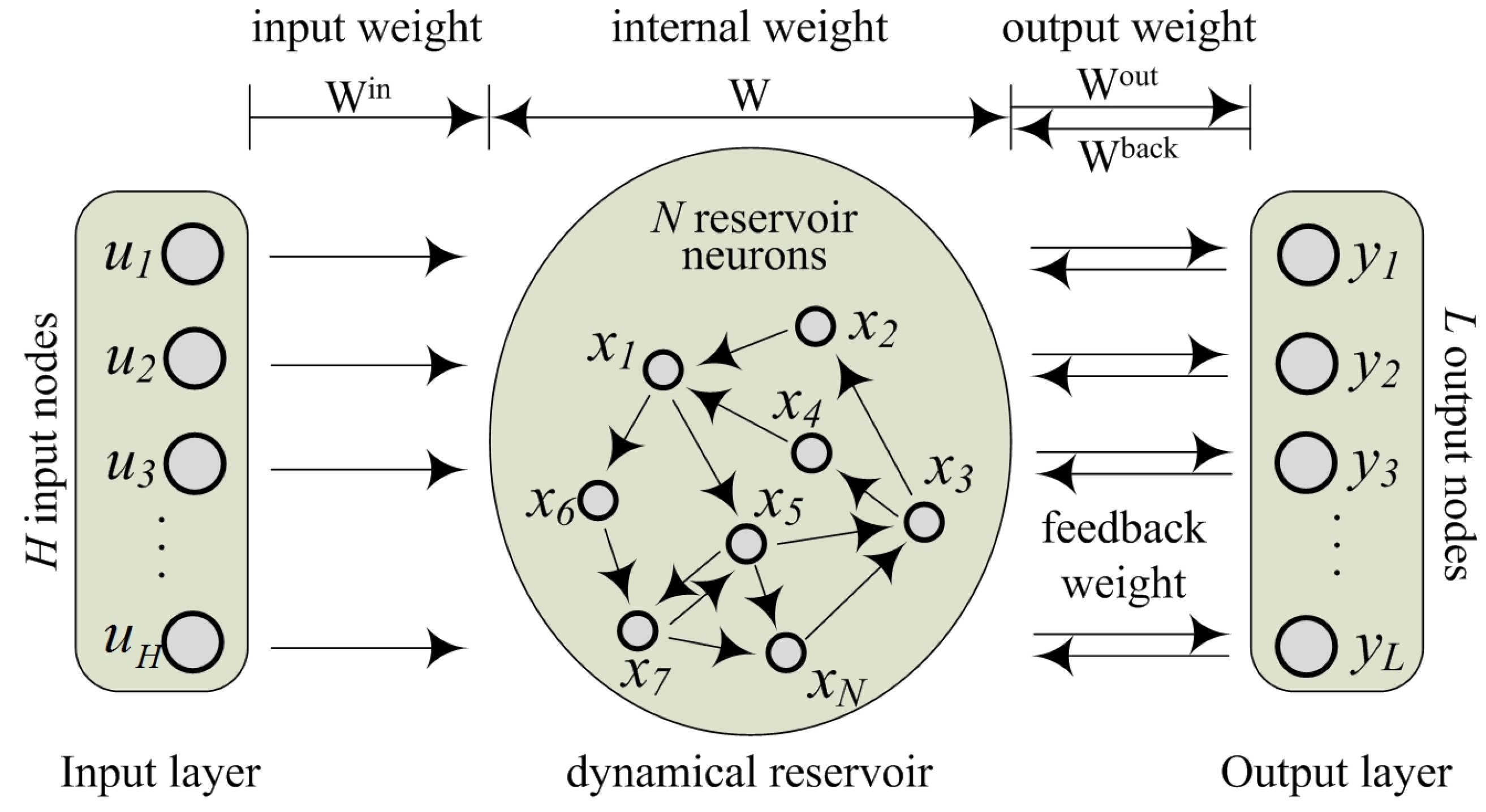
2.1. Echo State Network (ESN)

The generic ESN contains an input layer, a dynamical reservoir (DR) and an output layer, as illustrated in Figure 1. The DR is comprised of large sparsely and randomly connected neurons. Assuming the ESN includes H input nodes, N reservoir neurons and L output nodes, the status update of ESN reservoirs and readout can be expressed as Equations (1) and (2):

$$x(k)=f(W^{in}u(k)+Wx(k-1)+W^{back}y(k-1))$$

(1)

$$y(k)=f^{out}(W^{out}(u(k),x(k)))$$

(2)

where H is the number of input nodes; N is the number of neurons in the DR; and L is the number of the output nodes. At the kth step, $u(k)={[u_1(k),u_2(k),\dots ,u_H(k)]}^T$ is the input vector, $x(k)={[x_1(k),x_2(k),\dots ,x_N(k)]}^T$ is the states of DR, and $y(k)={[y_1(k),y_2(k),\dots ,y_L(k)]}^T$ is the output vector. $W^{in}$ is the input weight matrix representing the connectivity between input layer and reservoir neurons; $W$ is the weight matrix among the internal reservoir units. In order to provide sufficient memory capabilities, $W$ is a sparse matrix whose connectivity level keeps about 1%–5% and the spectral radius is less than 1; $W^{back}$ denotes the feedback weight matrix between output layer and reservoir neurons; $W^{out}$ denotes the output weight matrix. $f(\cdot )$ denotes the activation function of the internal neurons, and $f^{out}(\cdot )$ denotes the activation function of the output nodes. Once the input weight matrix $W^{in}$, internal weight matrix $W$ and feedback weight matrix $W^{back}$ are initialized, their values are not changed during the process of learning and testing and only the output weight matrix $W^{out}$ are trainable by the samples data set during the training process.

Therefore, the key of modeling an ESN is mainly about calculation of the output weight matrix. The linear regression algorithm is usually employed in order to obtain $W^{out}$.

$$W^{out}=M^{-1}T$$

(3)

where $M={[x{(T_0)}^T,x{(T_0+1)}^T,\cdots ,x{(T)}^T]}^T$ is the input and reservoir states matrix and $T={[y(T_0),y(T_0+1),\cdots ,y(T)]}^T$ is the teacher collection matrix. $T_0(T_0<T)$ is the initial time of the network.

The unstable solutions (3) sometimes occur due to the linear regression algorithm adopted to train the parameters. Through many experiments, the output weights can be of the order of 1 × 10⁸ or higher while very large values imply a lack of generalization capabilities [13]. Hence, the determination of the ESN output weights should be improved.

Figure 1. The architecture of standard Echo State Network (ESN).

Figure 1. The architecture of standard Echo State Network (ESN).

2.2. Bayesian Echo State Network (BESN)

For the given input, state of DR $x$ and desired output $t$, the error sum of squares $E_D=\frac{1}{2}{\displaystyle \sum _{i=1}^n{(f(z_i;W^{out})-t_i)}^2}$ is selected as the performance evaluation function. In this paper, the regularization item $E_W=\frac{1}{2}{\displaystyle \sum _{i=1}^L{(W^{out})}^2}$ is introduced into the performance evaluation function on the basis of regularization technique. Hence, the error function can be obtained as follows:

$$F(W^{out})=\text{β}{E}_D+\text{α}{E}_W$$

(4)

where α and β are the hyper-parameters. n is the size of data sample.

In the training process, the sample data, indicated as $\{(u_i,t_i)|i=1,\cdots ,T\}$, are trained. After settling the input u, state of DR x and desired output t, we can get a series of data pairs $\{(z_i,t_i)|i=1,\cdots ,n\}$. Then the output weight matrix is estimated by Bayesian method.

Bayesian theory focuses on the probability distribution of weight in the weight space [17]. The conventional learning process is started with a suitable prior probability distribution of the output weights $p(W^{out})$, before the observed data is obtained. Given the sample set, Bayes’ theorem is used for writing an expression of the posterior probability distribution for the output weights as follows:

$$p(W^{out}|D)=\frac{p(D|W^{out})p(W^{out})}{p(D)}$$

(5)

where $p(D|W^{out})$ is likelihood function; the denominator $p(D)$ is a normalization factor.

Suppose that $p(W^{out})$ obeys the common Gaussian distribution. Similarly, the likelihood function can be expressed in terms of error function $E_D$, and the posterior probability distribution of weights can be obtained in the form by:

$$p(W^{out}|D)=\frac{1}{Z_M(\text{α},\text{β})}\exp (-\text{β}{E}_D-\text{α}{E}_W)=\frac{1}{Z_M}\exp [-F(W^{out})]$$

(6)

where $Z_M(\text{α},\text{β})$ is not related to $W^{out}$. Therefore, the optimal output network weights can be trained by minimizing the error function $F(W^{out})$ or maximizing the posterior distribution $p(W^{out}|D)$. More details of Bayesian theory can be found in [18,19].

2.3. Hyper-Parameters Selection

The BESN has two hyper-parameters, of which α controls the prior distribution of output weight, and β controls the distribution of likelihood function. On the basis of Laplace approximation [19], the posterior probability distribution of network output weights can be approximately written as $p(w|D)=p(w|{\text{α}}^{*},{\text{β}}^{*},D)$, where ${\text{α}}^{*}$ and ${\text{β}}^{*}$ are the optimal values. So ${\text{α}}^{*}$ and ${\text{β}}^{*}$ are needed to obtain in order to maximize the posterior probability of output weights. According to [19,20,21], the optimal values of the hyper-parameters are:

$$\begin{array}{l}{\text{α}}^{*}=\frac{\text{γ}}{2E_W}\\ {\text{β}}^{*}=\frac{n-\text{γ}}{2E_D}\end{array}$$

(7)

where $\text{γ}={\displaystyle \sum _{i=1}^L\frac{{\text{λ}}_i}{{\text{λ}}_i+\text{α}}}$ and ${\text{λ}}_i$ is the eigenvalue of the Hessian matrix of the error function $E_D$.

2.4. Forecasting Steps of Power Production for SHP Plants

The forecasting steps for the power production of SHP plants by using the proposed BESN model are summarized as follows.

Step 1: Set the structure of the BESN model and initialize the weights $W^{in}$, $W$ and $W^{back}$.

Step 2: According to the sample data and Equation (1), calculate the states of DR.

Step 3: Initialize the hyper-parameters α and β, and the output weights $W^{out}$ of BESN.

Step 4: Compute the error function $F(W^{out})$ based on the hyper-parameters $\text{α}$ and $\text{β}$, and the output weights $W^{out}$.

Step 5: Optimize the output weight matrix via minimizing $F(W^{out})$ by using the Levenberg-Marquardt algorithm.

Step 6: Calculate $E_W$ and $E_D$ by using the current output weights $W^{out}$, and update the hyper-parameters α and β using Equation (7).

Step 7: Check whether the process of network training is completed or not. If completed, go to step 8; otherwise, go back to step 4.

Step 8: With the optimal output weights $W^{out}$ of BESN, the prediction procedure can be carried out by using Equations (1) and (2).

3. Overall Analysis and Study Area

3.1. Overall Analysis

At the end of 2013, China had more than 45,000 SHP plants with a total installed capacity of more than 68 GW with an annual generation over 200 TWh [1]. Most of the SHP plants are considered as “run-of-the-river” type, which have little or no reservoir regulation capacity. Their power production is mainly affected by natural factors, such as rainfall and inflow. For various reasons, not all of the necessary information, such as inflow for each SHP plant, can be obtained for forecasting short-term power production. Furthermore, due to numerous plants, even though the forecasting model could be established for only a single plant once and thus carried out one by one, the prediction workload would become very large, not to mention that the forecasting accuracy, which might not be able to meet the requirements.

In addition, all of the SHP plants in the same region are similar in terms of their hydrological and meteorological conditions, and their power generation processes are almost the same. Meanwhile, the power production of most of the plants in the same region can be transferred to the main power grid via the same transmission line, since each plant is integrated by different voltage levels. In other words, this influences the safe and stable operation of the power grid for all SHP plants within this region.

Therefore, in this paper, all of the SHP plants in the same region are selected and considered as a whole to establish a forecasting model. Considering successively putting into operation of SHP plants or hydro units, it is difficult to get satisfactory forecasting results, because the installed capacity in the single plant or the same region may vary from one day to another. To overcome this disadvantage, the installed capacity utilization hours are used as an indicator to denote power production of SHP plants in the region [4].

3.2. Study Area and Data

The Yunnan province, located in southwestern China, is extremely rich in hydropower resources. By the end of October, 2014, the number of SHP plants in Yunnan had reached 1595, with an installed capacity of 9168.59 MW, mainly distributed in the Dehong, Baoshan and Lincang regions in the southwest of the province, the Diqing and Nujiang regions in the northwest, and the Honghe and Wenshan regions in the south and southeast. At the same time, some large and medium-sized hydropower stations also exist in these regions. The SHP plants must share the same transmission resources with them to deliver and transmit power production. Due to lack of sufficient transmission capability, network congestion is likely to occur during the flood season. The two counties, Gongshan county and Zhenkang county, which are in Nujiang region and Lincang region respectively, are selected as study areas in this paper. At the end of October 2014, the Gongshan county had 12 SHP plants, with an installed capacity of 245.2 MW and Zhenkang county has 13 small hydropower plants with an installed capacity of 142.82 MW. The annual average temperature and annual average rainfall in Gongshan county are 16 °C and 2700–4700 mm, respectively, while 18.7 °C and 1625.4 mm in Zhenkang county.

In the present study, the daily observed data, including power production and rainfall, for 1280 days (from 1 May 2011 to 31 October 2014) are derived from both counties for this purpose, out of which 1219 days (from 1 May 2011 to 31 August 2014) are used for training and the rest are used for testing.

4. Application

4.1. Input Determination

Reasonably selecting input parameters may be helpful to capture the nonlinear features underlying the process and lead to good model performance. Considering the similarity of meteorological conditions in the same region over a period of a few days, the daily power production of SHP plants for a particular day should be near to the values of the day before and a few days hereafter. At the same time, since most of SHP plants are run-of-the-river plant with little or no reservoir regulation capacity, their power production is mainly influenced by rainfall on the current day or previous day. Therefore, to detect the proposed BESN model performance for forecasting power production of SHP plants in the two counties, all sub-series derived from the following five combinations: (i) G_t, G_t−1 and R_t, (ii) G_t, G_t−1, G_t−2 and R_t (iii) G_t, G_t−1, G_t−2, G_t−3 and R_t (iv) G_t, G_t−1, G_t−2, G_t−3 and R_t, $R_{t-1}$ (v) G_t, G_t−1, G_t−2, G_t−3, G_t−4 and R_t, R_t−1 are considered as inputs. G_t and R_t are power production and rainfall at day t, respectively. For a comparative purpose, the same input combinations are selected as inputs for LM-FNN and ESN. All the models employed in this study are implemented as Matlab codes.

In this paper, the following two statistical measures, root mean squared error (RMSE) and mean absolute percentage error (MAPE) given in Equations (14) and (15), are employed to evaluate the accuracy of forecasting results.

$$RMSE=\sqrt{\frac{1}{n}{\displaystyle \sum _{d=1}^n{\left(Energ{y}_d-Energ{y}_d^{*}\right)}^2}}$$

(8)

$$MAPE=\frac{1}{n}{\displaystyle \sum _{d=1}^n\left|\frac{Energ{y}_d^{*}-Energ{y}_d}{Energ{y}_d^{*}}\right|}\times 100$$

(9)

where $n$ is the total number of observed data, and $Energ{y}_d^{*}$ and $Energ{y}_d$ are, respectively, observed and forecasted value at day $d$.

4.2. Model Development

The feed-forward neural networks (FNN) is usually employed in hydrological forecasting, and many applications show that three layered FNN can yield satisfactory forecast results [22,23,24,25,26,27]. In this study, the LM-FNN with three layered architecture is selected as a benchmark model, for which the weight and bias values are updated by using Levenberg-Marquardt (LM) algorithm [28,29]. The primary task of establishing a LM-FNN model is to find an appropriate architecture that captures the relationship between the input and output variables. The main task of determining the appropriate architecture of the LM-FNN model is to confirm the number of nodes in the hidden layer because of the input combinations and the output being determined. The best hidden nodes number can be selected by varying the number from 3–15 by using the trial and error method. In addition, the number of iterations is used as convergence criteria, which is set as 1000.

For each LM-FNN model using the different input combinations mentioned, five training experiments with varied hidden nodes number are carried out and the best one according to their training performances is selected. The performance statistics of LM-FNN model of the SHP plants in the two counties are given in Table 1 and Table 2. The results clearly indicate that the most appropriate architectures of the LM-FNN for Gongshan county and Zhenkang county are (3, 8, 1) and (3, 7, 1), respectively.

Table 1. Performance statistics of Levenberg-Marquardt algorithm (LM-FNN) models for Gongshan county.

Model Inputs	Model Architecture	Calibration		Validation
		RMSE	MAPE	RMSE	MAPE
(i) Gt, Gt−1 and Rt	(3, 8, 1)	62.37	9.76	83.70	4.76
(ii) Gt, Gt−1, Gt−2 and Rt	(4, 7, 1)	65.34	10.09	87.48	4.97
(iii) Gt, Gt−1, Gt−2, Gt−3 and Rt	(5, 7, 1)	67.94	10.54	90.79	5.11
(iv) Gt, Gt−1, Gt−2, Gt−3 and Rt, Rt−1	(6, 8, 1)	66.38	10.41	88.01	4.96
(v) Gt, Gt−1, Gt−2, Gt−3, Gt−4 and Rt, Rt−1	(7, 9, 1)	70.43	11.19	90.53	5.10

Table 1. Performance statistics of Levenberg-Marquardt algorithm (LM-FNN) models for Gongshan county.

Model Inputs	Model Architecture	Calibration		Validation
		RMSE	MAPE	RMSE	MAPE
(i) Gt, Gt−1 and Rt	(3, 8, 1)	62.37	9.76	83.70	4.76
(ii) Gt, Gt−1, Gt−2 and Rt	(4, 7, 1)	65.34	10.09	87.48	4.97
(iii) Gt, Gt−1, Gt−2, Gt−3 and Rt	(5, 7, 1)	67.94	10.54	90.79	5.11
(iv) Gt, Gt−1, Gt−2, Gt−3 and Rt, Rt−1	(6, 8, 1)	66.38	10.41	88.01	4.96
(v) Gt, Gt−1, Gt−2, Gt−3, Gt−4 and Rt, Rt−1	(7, 9, 1)	70.43	11.19	90.53	5.10

Table 2. Performance statistics of LM-FNN models for Zhenkang county.

Model Inputs	Model Architecture	Calibration		Validation
		RMSE	MAPE	RMSE	MAPE
(i) Gt, Gt−1 and Rt	(3, 7, 1)	108.78	7.94	88.91	3.84
(ii) Gt, Gt−1, Gt−2 and Rt	(4, 5, 1)	111.92	8.08	84.03	3.97
(iii) Gt, Gt−1, Gt−2, Gt−3 and Rt	(5, 9, 1)	113.59	7.58	95.69	4.59
(iv) Gt, Gt−1, Gt−2, Gt−3 and Rt, Rt−1	(6, 8, 1)	116.16	7.78	94.54	4.04
(v) Gt, Gt−1, Gt−2, Gt−3, Gt−4 and Rt, Rt−1	(7, 9, 1)	124.95	8.55	106.39	4.72

Table 2. Performance statistics of LM-FNN models for Zhenkang county.

Model Inputs	Model Architecture	Calibration		Validation
		RMSE	MAPE	RMSE	MAPE
(i) Gt, Gt−1 and Rt	(3, 7, 1)	108.78	7.94	88.91	3.84
(ii) Gt, Gt−1, Gt−2 and Rt	(4, 5, 1)	111.92	8.08	84.03	3.97
(iii) Gt, Gt−1, Gt−2, Gt−3 and Rt	(5, 9, 1)	113.59	7.58	95.69	4.59
(iv) Gt, Gt−1, Gt−2, Gt−3 and Rt, Rt−1	(6, 8, 1)	116.16	7.78	94.54	4.04
(v) Gt, Gt−1, Gt−2, Gt−3, Gt−4 and Rt, Rt−1	(7, 9, 1)	124.95	8.55	106.39	4.72

The input weight Wⁱⁿ, w and W^back of the generic ESN model are randomly generated. On the basis of experiment, the number of neurons in the DR, sparse interconnectivity of DR and spectral radius of W are set as 100, 5% and 0.85, respectively. Hence, W is the 100 × 100 reservoir weight matrix and W^back is the 100 × 1 output feedback matrix. The BESN model employs the same network architecture of the generic ESN model, and its network parameters are similar to the proposed ESN model. However, the initial value of hyper-parameters is empirically set as α = 5 and β = 2.

The performance statistics of the ESN and BESN models in the two counties are given in Table 3 and Table 4. From the results, it can be easily seen that the most appropriate input combination of the ESN and BESN models for Gongshan county are (iii) and (i), respectively. For Zhenkang county, the most appropriate input combination are (ii) and (i), respectively. Thus, for the BESN models for the two counties, Wⁱⁿ is the 100 × 3 input weight matrix and W^out is the 1 × 103 output weight matrix. However, for the ESN models for Gongshan county and Zhenkang county, Wⁱⁿ are the 100 × 5 and 100 × 4 input weight matrix, and W^out are the 1 × 105 and 1 × 104 output weight matrix, respectively.

Table 3. Performance statistics of echo state network (ESN) and ESN with Bayesian regularization (BESN) models for Gongshan county.

Model Inputs	ESN				BESN
	Calibration		Validation		Calibration		Validation
	RMSE	MAPE	RMSE	MAPE	RMSE	MAPE	RMSE	MAPE
(i) Gt, Gt−1 and Rt	54.57	4.55	38.99	1.95	38.22	3.58	28.86	1.46
(ii) Gt, Gt−1, Gt−2 and Rt	56.43	5.08	41.79	2.01	39.15	3.66	29.39	1.47
(iii) Gt, Gt−1, Gt−2, Gt−3 and Rt	53.89	4.98	38.70	1.96	40.28	3.86	29.25	1.46
(iv) Gt, Gt−1, Gt−2, Gt−3 and Rt, Rt−1	56.63	5.23	39.19	2.02	39.20	3.89	30.78	1.56
(v) Gt, Gt−1, Gt−2, Gt−3, Gt−4 and Rt, Rt−1	55.56	4.97	41.12	2.01	40.08	3.69	30.86	1.57

Table 3. Performance statistics of echo state network (ESN) and ESN with Bayesian regularization (BESN) models for Gongshan county.

Model Inputs	ESN				BESN
	Calibration		Validation		Calibration		Validation
	RMSE	MAPE	RMSE	MAPE	RMSE	MAPE	RMSE	MAPE
(i) Gt, Gt−1 and Rt	54.57	4.55	38.99	1.95	38.22	3.58	28.86	1.46
(ii) Gt, Gt−1, Gt−2 and Rt	56.43	5.08	41.79	2.01	39.15	3.66	29.39	1.47
(iii) Gt, Gt−1, Gt−2, Gt−3 and Rt	53.89	4.98	38.70	1.96	40.28	3.86	29.25	1.46
(iv) Gt, Gt−1, Gt−2, Gt−3 and Rt, Rt−1	56.63	5.23	39.19	2.02	39.20	3.89	30.78	1.56
(v) Gt, Gt−1, Gt−2, Gt−3, Gt−4 and Rt, Rt−1	55.56	4.97	41.12	2.01	40.08	3.69	30.86	1.57

Table 4. Performance statistics of ESN and BESN models for Zhenkang county.

Model Inputs	ESN				BESN
	Calibration		Validation		Calibration		Validation
	RMSE	MAPE	RMSE	MAPE	RMSE	MAPE	RMSE	MAPE
(i) Gt, Gt−1 and Rt	121.44	6.81	82.39	3.56	74.03	5.60	49.50	2.49
(ii) Gt, Gt−1, Gt−2 and Rt	124.26	6.50	69.06	3.31	78.98	5.68	52.68	2.68
(iii) Gt, Gt−1, Gt−2, Gt−3 and Rt	125.01	7.21	74.72	3.39	80.92	5.94	55.20	2.82
(iv) Gt, Gt−1, Gt−2, Gt−3 and Rt, Rt−1	125.98	6.84	74.12	3.50	78.51	5.78	53.28	2.72
(v) Gt, Gt−1, Gt−2, Gt−3, Gt−4 and Rt, Rt−1	126.83	6.58	94.78	4.40	80.51	5.86	56.57	2.90

Table 4. Performance statistics of ESN and BESN models for Zhenkang county.

Model Inputs	ESN				BESN
	Calibration		Validation		Calibration		Validation
	RMSE	MAPE	RMSE	MAPE	RMSE	MAPE	RMSE	MAPE
(i) Gt, Gt−1 and Rt	121.44	6.81	82.39	3.56	74.03	5.60	49.50	2.49
(ii) Gt, Gt−1, Gt−2 and Rt	124.26	6.50	69.06	3.31	78.98	5.68	52.68	2.68
(iii) Gt, Gt−1, Gt−2, Gt−3 and Rt	125.01	7.21	74.72	3.39	80.92	5.94	55.20	2.82
(iv) Gt, Gt−1, Gt−2, Gt−3 and Rt, Rt−1	125.98	6.84	74.12	3.50	78.51	5.78	53.28	2.72
(v) Gt, Gt−1, Gt−2, Gt−3, Gt−4 and Rt, Rt−1	126.83	6.58	94.78	4.40	80.51	5.86	56.57	2.90

4.3. Results and Discussion

In this study, in order to evaluate the model performance for forecasting short-term power production of the SHP plants, the daily power production time series data are derived from two study sites in different counties. Meanwhile, the two statistical measures are employed to evaluate the model performance.

For Gongshan county and Zhenkang county, the model RMSE and MAPE statistics for the calibration and validation period are summarized in Table 5 and Table 6, respectively. The results shown both in Table 5 and Table 6 reveal that the BESN model is superior to the ESN model and the LM-FNN model in respect of all the two measures, not only in the calibration period but also in validation period. In the validation period, the BESN model improved the ESN model with a 25.4% and 25.5% reduction for Gongshan county and a 28.3% and 12.4% reduction for Zhenkang county in RMSE and MAPE values, respectively. Meanwhile, the values of these two measures of the BESN forecast are near to 1/3 than the LM-FNN model. In the comparison between the ESN and LM-FNN model in the calibration and validation period, the ESN model obtains much better values in RMSE and MAPE than the LM-FNN model for Gongshan county. For Zhenkang county, the ESN model obtains better RMSE and MAPE values than the LM-FNN in validation, while the LM-FNN model obtains better RMSE value than the ESN in calibration.

Table 5. Model statistics over the calibration and validation period for Gongshan county.

Model	Model Inputs	Calibration		Validation
		RMSE	MAPE	RMSE	MAPE
LM-FNN	(i) Gt, Gt−1 and Rt	62.37	9.76	83.70	4.76
ESN	(iii) Gt, Gt−1, Gt−2, Gt−3 and Rt	53.89	4.98	38.70	1.96
BESN	(i) Gt, Gt−1 and Rt	38.22	3.58	28.86	1.46

Table 5. Model statistics over the calibration and validation period for Gongshan county.

Model	Model Inputs	Calibration		Validation
		RMSE	MAPE	RMSE	MAPE
LM-FNN	(i) Gt, Gt−1 and Rt	62.37	9.76	83.70	4.76
ESN	(iii) Gt, Gt−1, Gt−2, Gt−3 and Rt	53.89	4.98	38.70	1.96
BESN	(i) Gt, Gt−1 and Rt	38.22	3.58	28.86	1.46

Table 6. Model statistics over the calibration and validation period for Zhenkang county.

Model	Model Inputs	Calibration		Validation
		RMSE	MAPE	RMSE	MAPE
LM-FNN	(i) Gt, Gt−1 and Rt	108.78	7.94	88.91	3.84
ESN	(ii) Gt, Gt−1, Gt−2 and Rt	124.26	6.50	69.06	3.31
BESN	(i) Gt, Gt−1 and Rt	74.03	5.60	49.50	2.49

Table 6. Model statistics over the calibration and validation period for Zhenkang county.

Model	Model Inputs	Calibration		Validation
		RMSE	MAPE	RMSE	MAPE
LM-FNN	(i) Gt, Gt−1 and Rt	108.78	7.94	88.91	3.84
ESN	(ii) Gt, Gt−1, Gt−2 and Rt	124.26	6.50	69.06	3.31
BESN	(i) Gt, Gt−1 and Rt	74.03	5.60	49.50	2.49

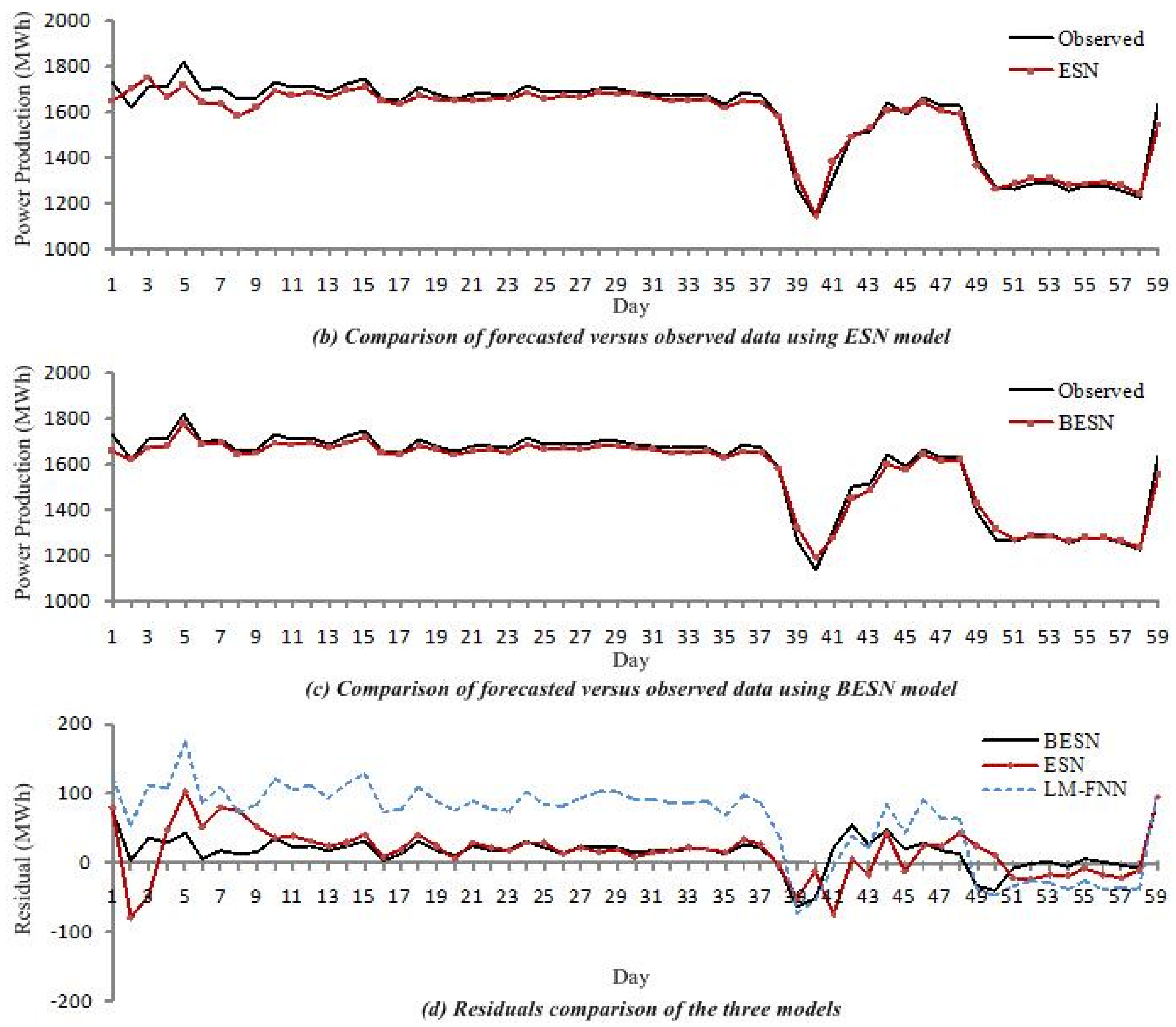
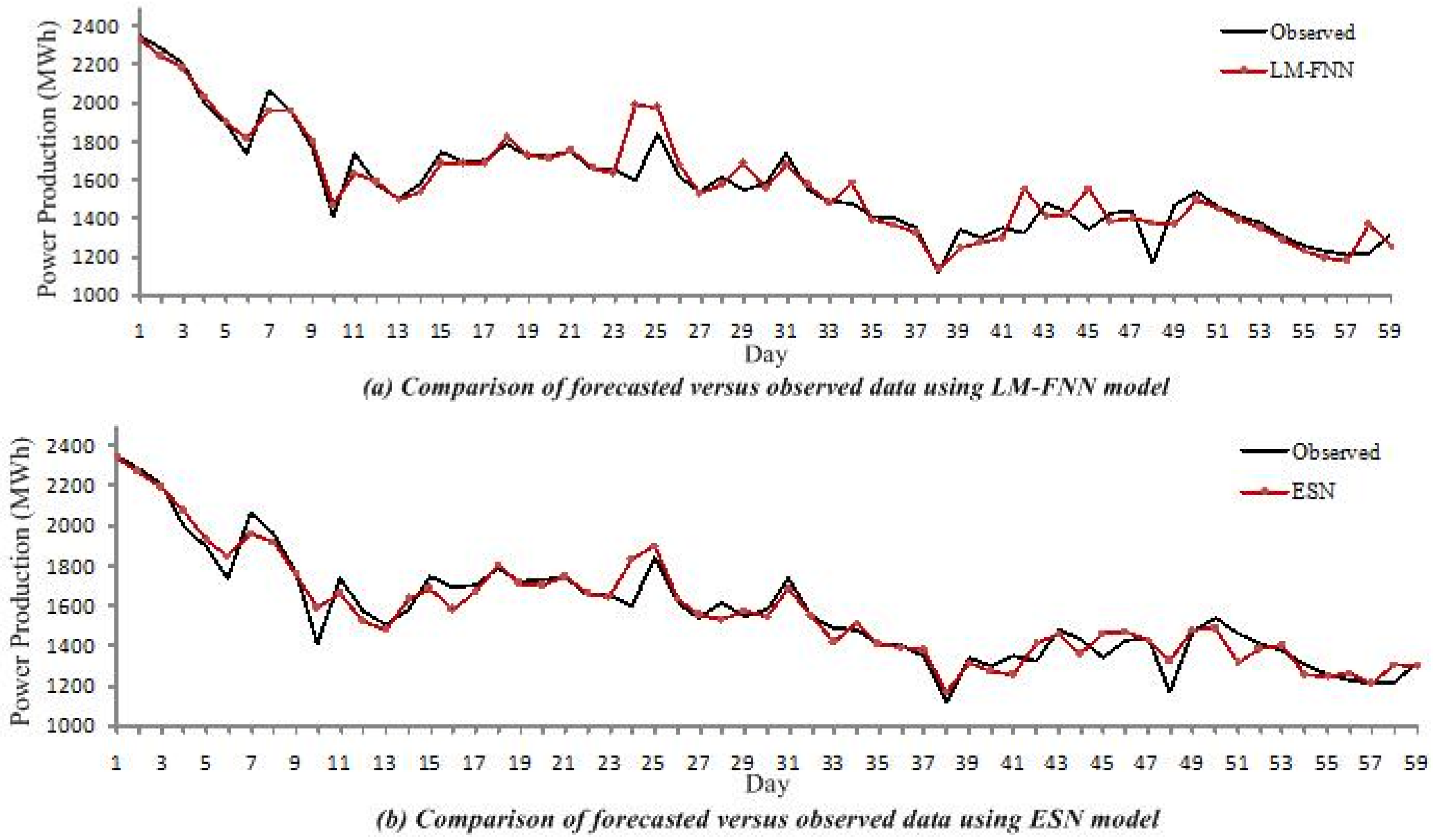
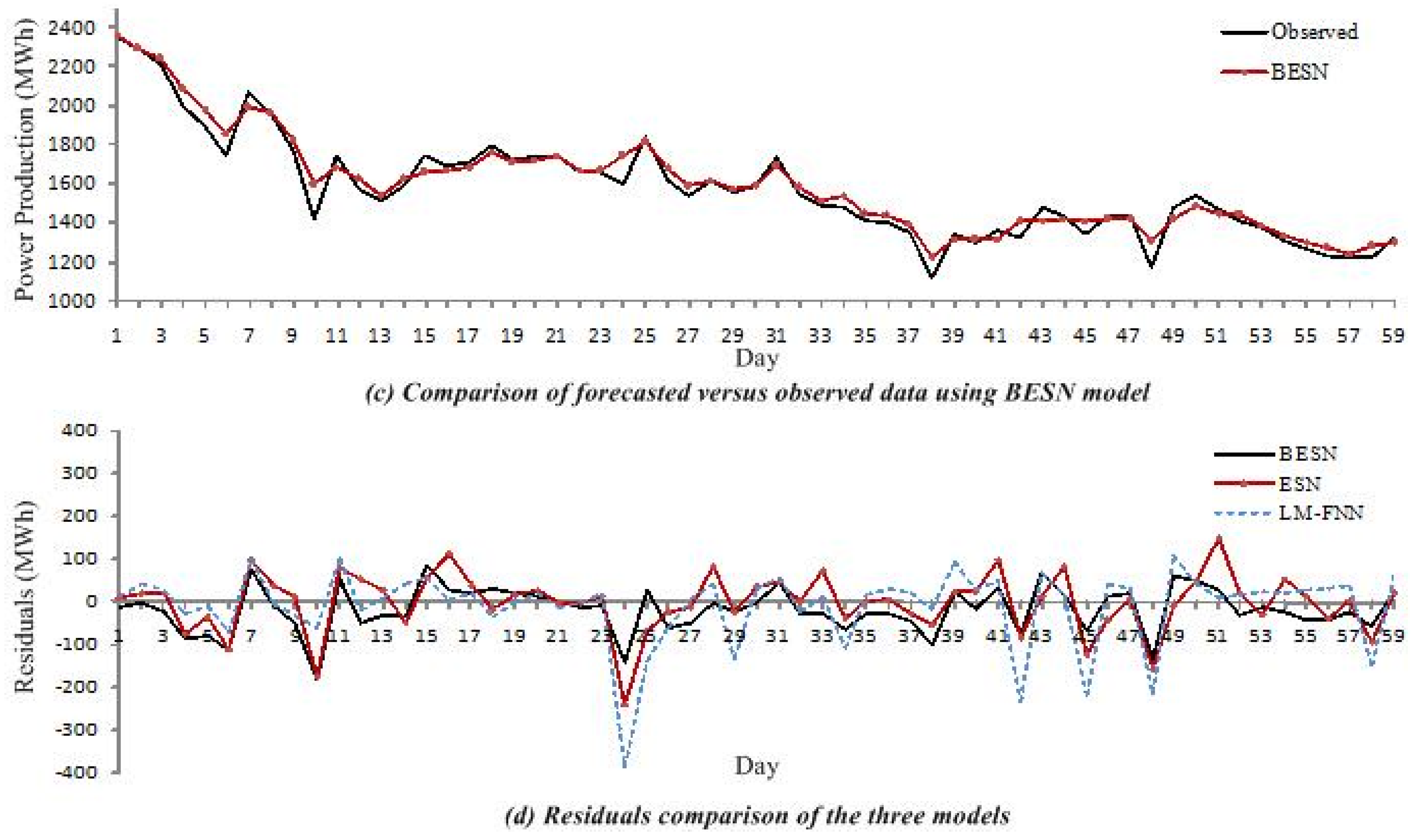
The comparison of forecasted versus observed data using BESN, ESN and LM-FNN model for Gongshan county and Zhenkang county are shown in Figure 2 and Figure 3, respectively. It can be easily seen that the forecast curve shape of the three models is similar to observed curve and the BESN model performs much better than both ESN and LM-FNN. Especially, at most of the inflection points, the BESN model shows better forecasting performance. From Figure 2, the LM-FNN model forecasts the maximum power production as 1641.69 MWh instead of observed 1815.24 MWh for Gongshan county, with an underestimation of 9.56%. The ESN model forecast the maximum power production as 1713.44 MWh with an overestimation of 5.61%; however, the BESN forecast the maximum power production as 1771.65 MWh with an overestimation of 2.40%. The same is true with Zhenkang county from Figure 3. Therefore, it can be concluded that the BESN model obtains slightly better forecast precision than the ESN model both at the inflection points and in the remaining part of the time series, while the BESN and ESN model obtain much better forecast precision than the LM-FNN model.

Figure 2. Comparison of forecasted versus observed data using LM-FNN, ESN and BESN model for Gongshan county.

Figure 2. Comparison of forecasted versus observed data using LM-FNN, ESN and BESN model for Gongshan county.

Figure 3. Comparison of forecasted versus observed data using LM-FNN, ESN and BESN model for Zhenkang county.

Figure 3. Comparison of forecasted versus observed data using LM-FNN, ESN and BESN model for Zhenkang county.

5. Conclusions

In the present study, the BESN model based on the echo state network with Bayesian regularization has been developed for forecasting short-term power production of SHP plants. The daily power production data derived from the Gongshan and Zhenkang counties in the Yunnan province, China, were employed to evaluate model performance of the BESN. In order to better assess the BESN model performance, the ESN and LM-FNN models were employed in a comparative manner. For all three models, the input determination was experientially based on five input combinations, because of the similarity of meteorological conditions a few days before and after the chosen day. The most appropriate input combination of the LM-FNN and BESN model was input (i) for each county; the ESN model was input (iii) and (ii) for the Gongshan and Zhenkang counties, respectively. Thereafter, the three models were constructed and their performances compared. The results demonstrate that the ESN model performs slightly better than the LM-FNN. Further, the BESN model obtained a more accurate forecast precision than both the ESN and LM-FNN models.

From the discussion above, we may safely draw a conclusion that the BESN model is a feasible tool for forecasting short-term power production of SHP plants, because its forecast precision could meet the dispatching operation requirement of a power system, which requires accuracies higher than 90%. As is well known, there are many classical and mature forecasting models that have been applied in hydrological prediction and these models warrant further study in the future.