Forecasting China’s Annual Biofuel Production Using an Improved Grey Model

Abstract

Biofuel production in China suffers from many uncertainties due to concerns about the government’s support policy and supply of biofuel raw material. Predicting biofuel production is critical to the development of this energy industry. Depending on the biofuel’s characteristics, we improve the prediction precision of the conventional prediction method by creating a dynamic fuzzy grey–Markov prediction model. Our model divides random time series decomposition into a change trend sequence and a fluctuation sequence. It comprises two improvements. We overcome the problem of considering the status of future time from a static angle in the traditional grey model by using the grey equal dimension new information and equal dimension increasing models to create a dynamic grey prediction model. To resolve the influence of random fluctuation data and weak anti-interference ability in the Markov chain model, we improve the traditional grey–Markov model with classification of states using the fuzzy set theory. Finally, we use real data to test the dynamic fuzzy prediction model. The results prove that the model can effectively improve the accuracy of forecast data and can be applied to predict biofuel production. However, there are still some defects in our model. The modeling approach used here predicts biofuel production levels based upon past production levels dictated by economics, governmental policies, and technological developments but none of which can be forecast accurately based upon past events.

1. Introduction

China’s biofuel industry has developed rapidly in recent years. On the one hand, China’s oil consumption is growing very fast, and China has overtaken the U.S. as the world’s largest oil importer [1]. From 2002 to 2013, China’s oil consumption increased sharply and was close to 500 million tons in 2013, with its overseas oil dependence ratio increasing to 58.8% [2]. By 2035, China is likely to account for about 15% of global oil consumption, which means that it is likely to record the world’s highest increase in oil imports in the coming decades [3]. Moreover, China’s domestic oil demand is projected to increase to 650,750 million tons and 750,750 million tons by 2030 and 2050, respectively [4]. Biofuels are increasingly considered as very important in addressing energy security problems, poverty reduction, and decreasing dependency on fossil fuels [5,6,7]. On the other hand, China has become the world’s top carbon dioxide (CO₂) producer [8]. With air pollution becoming an increasingly serious issue in China, the use of biofuels, which are essentially novel types of sustainable fuels, has attracted much attention as a way to reduce China’s smog and carbon emissions [5,6,7,8,9]. During the 2014, Asia-Pacific Economic Cooperation (APEC) Meeting in Beijing, Chinese President Xi Jinping and U.S. President Barack Obama jointly issued the China–U.S. Joint Statement on Climate Change. President Obama promised to reduce the U.S.’ carbon emissions by 26% to 28% by 2025 [10]. To achieve this goal, the global demand for biofuels in road transport is expected to rise from 32.4 billion gallons in 2013 to 51.1 billion gallons in 2022, a growth of nearly 60%. The Chinese government has been actively promoting the uptake of biofuels since 2000, recognizing them as a key strategic measure in addressing the challenges of climate change and energy security [11]. In 2010, China’s biofuels industry was listed as one of the national strategic emerging industries. According to the long-term development prospects of renewable energy, by 2020, biofuels could account for 15% of transportation energy consumption, with biofuels substituting 10% of conventional fuels [12]. Keeping these factors in mind and given the rise in China’s overall biofuel production from 2003 to 2012, it is important to devise accurate methods to see whether the production can actually achieve the long-term development of renewable energy.

2. Literature Review

2.1. Predicting Biofuel Production

A debate is now focused on the impact of meeting the 2020 carbon emission reduction targets. Some existing studies have analyzed this issue. For example, Chang et al. [13] conducted an assessment of potential technology pathways to achieve this goal and concluded that China can potentially satisfy its biofuel production target by 2020 from a technology perspective alone. Qiu et al. [14] argued that China’s target of producing 10 million tons of ethanol fuel by 2020 appears to be prudent and should cause no major disturbances to China’s food security. Tian et al. [15] claimed that if reserved land resources are explored with substitute planting and unit area yield improvements; bioethanol fuel production can meet the goal set for 2020. Wu [16], however, concluded that in the current scenario, China’s bioethanol production cannot meet domestic demand and that there is a huge gap between supply and demand. They opined that China has a long way to go before meeting its goal of producing 10 million tons of bioethanol fuel by 2020.

2.2. Problems with Predicting Production

Generally, the past literature has adopted traditional methods such as linear regression [17], expert systems [18], neural networks [19,20], and Markov prediction and factor analysis [21] for yield prediction. However, the biofuels system is a complex system, which is easily affected by various factors such as the economy, resources, and social issues. Traditional methods face the problems of sample shortages and difficult and voluminous calculations for production forecasting. Therefore, the traditional methods are not suitable for predicting biofuel production.

The grey system theory was devised by Deng [22,23] in the 1980s as an effective method to deal with the problems posed by small samples, poor information, and uncertainty. Grey prediction [24] is a prediction method based on the grey system theory, the basic idea being to accumulate the randomness and uncertainty of irregular historical data and then generate the law of exponential sequence followed by the establishment of the forecast model or the grey differential equation. To date, the grey forecasting model GM (1,1) has been widely used in many fields, such as energy production [25,26], electricity consumption, gas consumption [27,28], CO₂ emissions prediction, coal production [29], and photoelectric output [30], because it requires less data and offers certain advantages, including easy computation and high prediction accuracy. Like other mathematical models, the grey model should be used within its application range to avoid producing large errors. An improved GM (1,1) model, as described below, can not only enhance the accuracy of the prediction model but also increase its application potential.

In recent years, Truong and Ahn [31] modified the grey model to create the first-order one-variable modified grey model MGM (1,1) to predict wave parameters effectively. Liu et al. [32] developed an optimization model by improving the grey model and enhancing prediction accuracy after referring to initial and background values. Xie and Liu [33] proposed a novel discrete grey forecasting model, termed the DGM model, which increased the tendency catching ability of the model. Tien [34] proposed a new grey prediction model, called the first entry grey model or FGM (1,1), which inserted an arbitrary number n before the original series to extract messages from the first entry to forecast future data. Li et al. [35] proposed the trend and potency tracking method (TPTM) to construct a new optimized grey model, namely the adaptive grey prediction model or AGM (1,1), to obtain higher forecasting quality.

Some scholars have studied the grey prediction model combined with an algorithm such as the genetic algorithm [36], Verhulst power allocation [37], technique for order of preference by similarity to ideal solution (TOPSIS) [38], and particle swarm optimization (PSO) [39]. These studies dramatically improved the simulative error and prediction accuracy of the grey model.

The model proposed in this paper improves the prediction method from two aspects. First, it overcomes the weakness of the traditional grey model, which considers the future status from a static angle. We use the grey equal dimension new information model and the equal dimension increasing model to create the dynamic grey prediction model. To tackle the influence of random fluctuation data on forecasting accuracy in the Markov chain model and the limitation of weak anti-interference ability, we introduce the fuzzy set theory and improve the traditional grey–Markov model using classifications of states.

The conventional GM (1,1) model can only consider all real-time past data. However, with the passage of time, the old information will produce disturbances in systems intended for future/long-term predictions [40]. These issues cause a decline in prediction accuracy and prediction significance. A readymade GM (1,1) model for long-term forecasts, therefore, results in a reduction of prediction accuracy and fails to reflect changes in the system. Prediction reliability is thus very low. We need to be able to use all the given information comprehensively to reflect changes in the system and state, and if there is no given information, we can use grey information. In the former case, we use the grey equal dimension new information model, and in the latter, we employ the equal dimension grey increasing model [41]. Combining the two models can help us comprehensively utilize the actual data and grey information may be used as a timely supplement when there is no given information. This combination can also improve the prediction precision. Thus, in this article, the Markov chain combination forecast model is adopted to establish a state transition probability matrix and determine the forecast object transfer status to correct the forecasted results. This article first applies the conventional grey model and dynamic grey prediction model to China’s biofuel production data for 2002 to 2013 and compares their prediction accuracies. Then, the model with the higher accuracy is used to predict China’s biofuel production for the next 6 years (2015 to 2020).

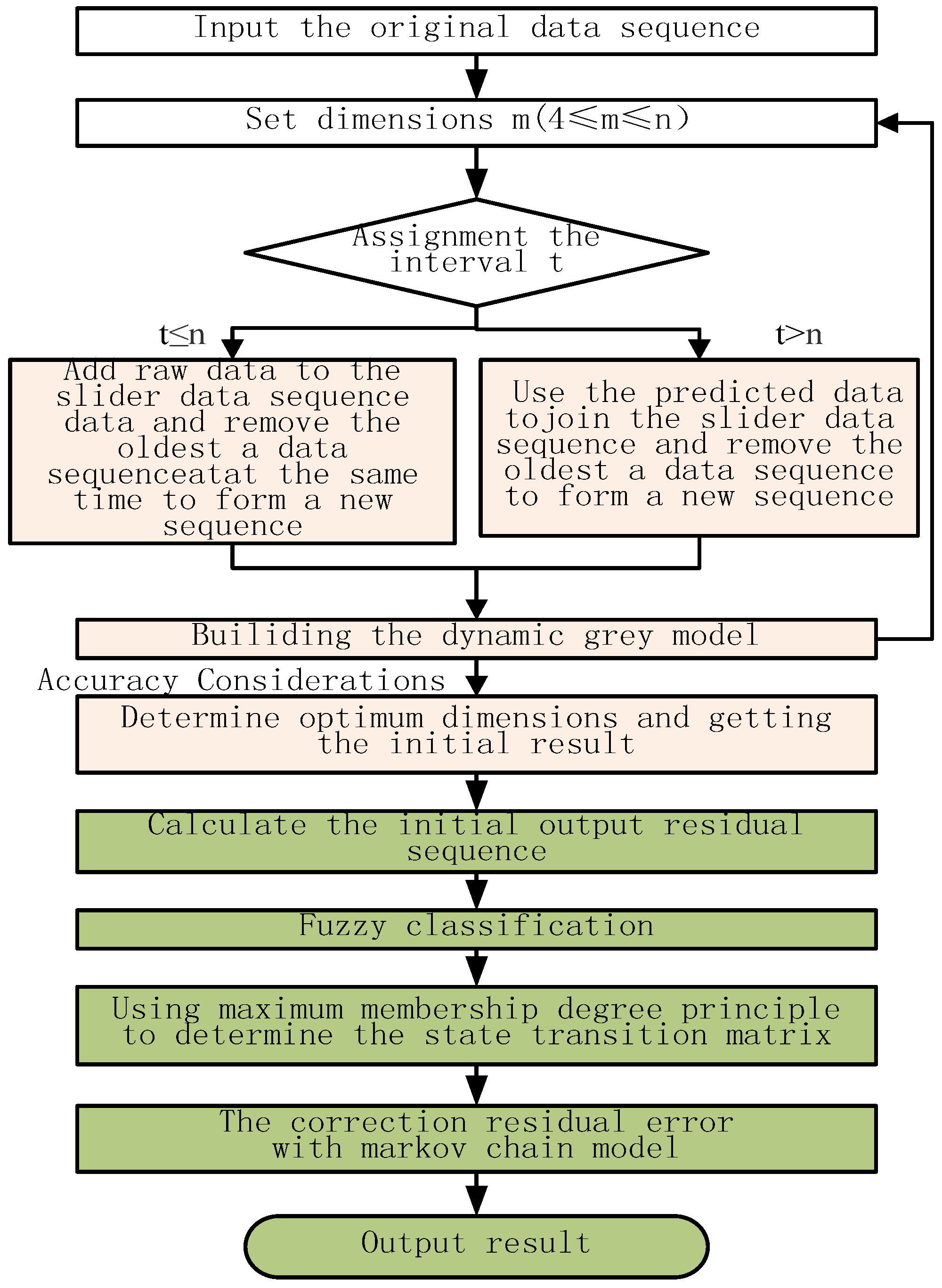
3. Building the Dynamic Grey Fuzzy Markov Prediction Model

The dynamic grey fuzzy Markov prediction model is an improvement on the conventional grey model.

3.1. Conventional Grey Model

3.1.1. GM (1,1) Model Building Process

The GM (1,1) model is the basic grey prediction model, which is composed of a first-order differential equation model with a single variable. The model building process comprises the following steps [22,23,24]:

• Accumulated generating operation (AGO)
• Grey modeling
• Inverse accumulated generating operation (IAGO)

Step 1: Establish the initial time sequence:

$$X^{(0)}=(x^{(0)}(1),x^{(0)}(2),\mathrm{...},x^{(0)}(n))$$

(1)

Here, $X^{(0)}$ is a non-negative sequence, and n is the number of the data.

Step 2: Subject the sequence from Step 1 to the AGO, and obtain sequence $X^{(1)}$:

$$X^{(1)}=(x^{(1)}(1),x^{(1)}(2),\mathrm{...},x^{(1)}(n))$$

(2)

Step 3: Establish a first-order grey differential equation:

$$x^{(1)}(k)+a{z}^{(1)}(k)=b$$

(3)

where:

$$z^{(1)}(k)=0.5x^{(1)}(k)+0.5x^{(1)}(k-1)$$

(4)

a is called the development coefficient, and b is called the driving coefficient. Applying the least squares method, coefficients [a, b] can be estimated as follows:

$$\stackrel{\wedge }{\alpha }=\left[\begin{array}{l}a\\ b\end{array}\right]={(B^{T}B)}^{-1}{B}^{T}Yn$$

(5)

where:

$$Y_n=\left[\begin{array}{c}{x}^{(0)}(2)\\ x^{(0)}(3)\\ \mathrm{...}\\ x^{(0)}(n)\end{array}\right]B=\left[\begin{array}{cc}-z^{(1)}(2)& 1\\ -z^{(1)}(3)& 1\\ \mathrm{...}& \mathrm{...}\\ -z^{(1)}(n)& 1\end{array}\right],Y_n=\left[\begin{array}{c}{x}^{(0)}(2)\\ x^{(0)}(3)\\ \mathrm{...}\\ x^{(0)}(n)\end{array}\right]$$

(6)

Step 4: Conduct the whitenization process using the grey differential equation in Equation (3). The process is essentially a transformation process, which means that it changes the grey system with partial unknown information and partial known information into a white system with completely certain information. It is defined mathematically as follows:

$$\frac{\text{d}{x}^{(1)}}{\text{d}t}+a{x}^{(1)}=b$$

(7)

Then, we use the least squares method to solve the above equations and get the GM (1,1) prediction model as follows:

$${\widehat{x}}^{(1)}(k+1)=[x^{(1)}(0)-\frac{b}{a}]e^{-ak}+\frac{b}{a},k=1,2,\mathrm{...},n$$

(8)

Step 5: Obtain the prediction value of the original sequence by IAGO. The IAGO can be defined as:

$${\widehat{x}}^{(0)}(k+1)={\widehat{x}}^{(1)}(k+1)-{\widehat{x}}^{(1)}(k)=(1-e^a)[x^{(1)}(0)-\frac{b}{a}]e^{-ak}$$

(9)

3.1.2. Accuracy Considerations

In order to inspect the accuracy of the GM (1,1) model, we need to test the prediction accuracy and posterior error of the model. We set the original sequence $X^{(0)}=\left\{x^{(0)}(1),x^{(0)}(2),\mathrm{...},x^{(0)}(n)\right\}$ in the corresponding model to simulate sequences. ${\widehat{X}}^{(0)}=\left\{{\widehat{x}}^{(0)}(1),{\widehat{x}}^{(0)}(2),\mathrm{...},{\widehat{x}}^{(0)}(n)\right\}$. The residual difference is ${\mathrm{\epsilon }}^{(0)}=\left\{\mathrm{\epsilon }(1),\mathrm{\epsilon }(2),\cdots ,\mathrm{\epsilon }(n)\right\}$$=\left\{x^{(0)}(1)-{\widehat{x}}^{(0)}(1),x^{(0)}(2)-{\widehat{x}}^{(0)}(2),\cdots ,x^{(0)}(n)-{\widehat{x}}^{(0)}(n)\right\}$. Thus, the relative error sequence is $\mathrm{\Delta }=\left\{\left|\frac{\mathrm{\epsilon }(1)}{x^{(0)}(1)}\right|,\left|\frac{\mathrm{\epsilon }(2)}{x^{(0)}(2)}\right|,\cdots ,\left|\frac{\mathrm{\epsilon }(n)}{x^{(0)}(n)}\right|\right\}$. $\overline{\mathrm{\Delta }}=\frac{1}{n}{\displaystyle \sum _{k=1}^n{\mathrm{\Delta }}_k}$ is denoted as the average relative error. $1-\overline{\mathrm{\Delta }}$ is denoted as the correctly predicted percentage. $\overline{x}=\frac{1}{n}{\displaystyle \sum _{k=1}^n{x}^{(0)}(k)}$ is the mean value of $X^{(0)}$, $s_1^2=\frac{1}{n}{\displaystyle \sum _{k=1}^n(x^{(0)}(k)}-\overline{x}{)}^2$ is the variance of $x^{(0)}$, $\overline{\mathrm{\epsilon }}=\frac{1}{n}{\displaystyle \sum _{k=1}^n\mathrm{\epsilon }(k)}$ is the mean of residual errors, $s_2^2=\frac{1}{n}{\displaystyle \sum _{k=1}^n{(\mathrm{\epsilon }(k)-\overline{\mathrm{\epsilon }})}^2}$ is the residual variance, $C=\frac{s_2}{s_1}$ is the mean square error ratio, and $P=\left\{|{\mathrm{\Delta }}_k-\overline{\mathrm{\Delta }}|\right\}\le 0.6745s_1$ is the minimum error probability. Precision inspection levels are shown in Table 1.

Table 1. Reference values for precision inspection levels.

Index		C	P
Accuracy grade	Excellent	≤0.35	≥95%
	Well	≤0.50	≥80%
	Conformity	≤0.65	≥70%
	Non-conformity	≥0.80	≤60%

Table 1. Reference values for precision inspection levels.

Index		C	P
Accuracy grade	Excellent	≤0.35	≥95%
	Well	≤0.50	≥80%
	Conformity	≤0.65	≥70%
	Non-conformity	≥0.80	≤60%

3.2. Dynamic Grey Model

The GM (1,1) model’s long-term prediction effectiveness is significantly affected by system time sequence length and data changes. If the data column applied to the system modeling process is too short, it is difficult to obtain a long-term forecast. However, if the data column is too long, the system interference of the ingredients is too high, thus increasing instability and reducing the model’s prediction accuracy. Therefore, while conducting a dynamic prediction, we add dimensions constraint conditions; namely, we first fix the length of the interval t, then, we use the special projections method with the actual value followed by the predicted value; we modify the model with every prediction; and last, we produce the predicted value in the dynamic process and improve the degree of the prediction fitting curve.

Assume that the original data is $X^{(0)}=(x^{(0)}(1),x^{(0)}(2),\mathrm{...},x^{(0)}(n))$. When t ≤ n, we improve the original GM (1,1) model on the basis of the observed data at time n + 1 (referred to as new interest rates). We take the original sequence $X^{(0)}$, remove $x^{(0)}(1)$, add $x^{(0)}(n+1)$ and then form a new dynamic sequence $\left\{x^{(0)}(2),x^{(0)}(3),\mathrm{...},x^{(0)}(n+1)\right\}$.

When t > n, we generate $X^{(1)}$ after one AGO and then create the GM (1,1) model. According to Equations (8) and (9) we get the projections ${\widehat{x}}^{(0)}(n+1)$ at time n + 1. Then, we delete $x^{(0)}(1)$, add grey numbers ${\widehat{x}}^{(0)}(n+1)$, and reconstitute an equi-dimensional series $\left\{x^{(0)}(2),x^{(0)}(3),\mathrm{...},{\widehat{x}}^{(0)}(n+1)\right\}$.

The steps described above are repeated to set up the GM (1,1) model, and we continue substituting predictions one by one to arrive at the dynamic grey prediction model. Through this method, we resolve the problem of bigger errors caused by less data in the equal dimension grey increasing model. At the same time, we also remedy the disadvantages of limited medium- and long-term predictions with limited actual data in the grey equal dimension new information model, thus improving the prediction accuracy.

3.3. Dynamic Grey Fuzzy Markov Prediction Model

This article uses the Markov method to correct the results of the predicted data sequence in the dynamic grey prediction model. In doing so, the article chooses relative error sequence as an object. ${\mathrm{\epsilon }}_k=\frac{x^{(0)}(k)-{\widehat{x}}^{(0)}(k)}{{\widehat{x}}^{(0)}(k)}(k=1,2,\mathrm{3...}n)$ is the relative magnitude of the residual error; a higher ${\mathrm{\epsilon }}_k$ refers to a larger deviation between the actual and tendency values. In this case, the stability worsens. In contrast, a lower. ${\mathrm{\epsilon }}_k$ refers to smaller deviations between the actual and tendency values, implying an improvement in stability. We call the resulting model the dynamic grey fuzzy Markov prediction model or DGFM (1,1).

3.3.1. Fuzzy Classifications

The system is divided into a state division as the standard of relative magnitude of the residual, and any state can be expressed as ${\mathrm{\Theta }}_i=\left[{\mathrm{\Theta }}_{i1},{\mathrm{\Theta }}_{i2}\right]$, i = 1,2…,m:

$${\mathrm{\Theta }}_{i2}=\frac{{\widehat{x}}^{(0)}(k)}{1-{\text{δ}}_1},{\mathrm{\Theta }}_{i1}=\frac{{\widehat{x}}^{(0)}(k)}{1-{\text{δ}}_{i-1}},{\mathrm{\Theta }}_{i2}=\frac{{\widehat{x}}^{(0)}(k)}{1-{\text{δ}}_1}$$

(10)

In the above formula, ${\text{δ}}_{i-1}$ and ${\text{δ}}_1$ are the upper and lower boundaries, which are the standards of the relative residual error, whereas and ${\mathrm{\Theta }}_{i1}$ and ${\mathrm{\Theta }}_{i2}$ are the upper and lower boundaries of the i state value. For a relative residual, ($U$ $x\in U$, ($U$ is the relative residual set)), each membership function of the fuzzy set method (triangle) can be expressed as:

$$\begin{array}{l}{u}_1(x)=\{\begin{array}{cc}1\hfill & {\text{δ}}_0\le x\le \frac{{\text{δ}}_0+{\text{δ}}_1}{2}\\ \frac{{\text{δ}}_1+{\text{δ}}_2-2x}{{\text{δ}}_2-{\text{δ}}_0}\hfill & \frac{{\text{δ}}_0+{\text{δ}}_1}{2}\le x\le \frac{{\text{δ}}_1+{\text{δ}}_2}{2},i\ne 1,m\\ 0\hfill & \text{others}\end{array}\end{array}$$

(11)

$$\begin{array}{l}{u}_i(x)=\{\begin{array}{cc}\frac{2x-{\text{δ}}_{i-2}-{\text{δ}}_{i-1}}{{\text{δ}}_i-{\text{δ}}_{i-2}}\hfill & \frac{{\text{δ}}_{i-2}+{\text{δ}}_{i-1}}{2}\le x\le \frac{{\text{δ}}_{i-1}+{\text{δ}}_i}{2}\hfill \\ \frac{{\text{δ}}_{i+1}-{\text{δ}}_{i-1}-2x}{{\text{δ}}_{i+1}-{\text{δ}}_{i-1}}\hfill & \frac{{\text{δ}}_{i-1}+{\text{δ}}_i}{2}\le x\le \frac{{\text{δ}}_i+{\text{δ}}_{i+1}}{2},i\ne 1,m\\ 0\hfill & \text{others}\end{array}\end{array}$$

(12)

$$u_m(x)=\{\begin{array}{cc}\frac{2x-{\text{δ}}_{m-2}-{\text{δ}}_{m-1}}{{\text{δ}}_m-{\text{δ}}_{m-2}}\hfill & \frac{{\text{δ}}_{m-2}+{\text{δ}}_{m-1}}{2}\le x\le \frac{{\text{δ}}_{m-1}+{\text{δ}}_m}{2}\\ 1\hfill & \frac{{\text{δ}}_{m-1}+{\text{δ}}_m}{2}\le x\le {\text{δ}}_m\\ 0\hfill & \text{others}\end{array}$$

(13)

3.3.2. Determination of the State Transition Matrix

Using the maximum membership degree principle, we determine the relative state of each residual relative magnitude. For any relative residual $x\in U$, the existing k₀ makes $U_{k_0}(x)=\underset{k=1}{\overset{m}{\vee }}\left\{u_{A_k}(x)\right\},1\le k_0\le m.$ Then, we regard $A_{k0}$ as x’s relative membership degree. A₁, A₂, …, A_m are m fuzzy subsets on U. The state transition probability is $p_{ij}=\frac{M_{ij}}{M_i},i=1,\mathrm{2...}n$, where $M_{ij}$ is the frequency that state ${\mathrm{\Theta }}_i$ reaches state ${\mathrm{\Theta }}_j$ after the Step 1 transfer, and $M_i$ is the occurrence frequency of ${\mathrm{\Theta }}_i$. $P$ is the transition probability matrix.

3.3.3. Fuzzy Markov Residual Error Correction

$\text{δ}(n)$ is the relative residual value at time n, and $u_A(\text{δ}(n))$ is the membership of $\text{δ}(n)$ about every fuzzy state $F(\text{δ}(n))=(u_{A_1}(\text{δ}(n)),u_{A2}(\text{δ}(n)),\mathrm{...},u_{A_m}(\text{δ}(n)))$. The relative residual error sequence at time (t + 1) is still a fuzzy vector, that is, where $F(\text{δ}(n+1))$ $F(\text{δ}(n+1))=F(\text{δ}(n))P=(u_{A_1}(\text{δ}(n+1)),u_{A2}(\text{δ}(n+1)),\mathrm{...},u_{A_m}(\text{δ}(n+1)))$, where $F(\text{δ}(n+1))$ refers to the relative residual estimate for each membership degree of the fuzzy state at (t + 1). Using the weighted sum method gives us $\text{δ}(n+1)={\displaystyle \sum _{i=1}^m\frac{1}{2}}{u}_{A_i}(\text{δ}(n))({\text{δ}}_{i-1}+{\text{δ}}_i)$, and then, the forecast for (n + 1) is ${\stackrel{\wedge }{y}}^{(0)}(n+1)=\frac{{\stackrel{\wedge }{x}}^{(0)}(n+1)}{1-\delta (n+1)}$. Figure 1 depicts the process diagram of the dynamic grey fuzzy Markov prediction model.

Figure 1. Process diagram of the dynamic grey fuzzy Markov prediction model.

Figure 1. Process diagram of the dynamic grey fuzzy Markov prediction model.

4. Feasibility Analysis of the Grey Fuzzy Markov Prediction Model

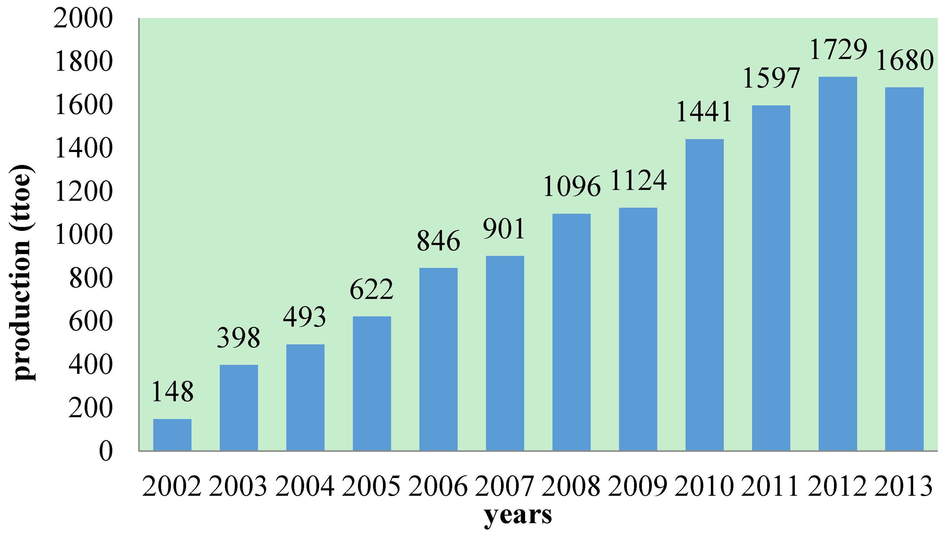
4.1. Data Source

China’s biofuel production statistics from 2002 to 2013 are sourced from BP World Energy Statistical Yearbook [42]. The total biofuel output for China shows an increasing trend over the studied period (Figure 2).

Figure 2. China’s biofuel production from 2002 to 2013.

Figure 2. China’s biofuel production from 2002 to 2013.

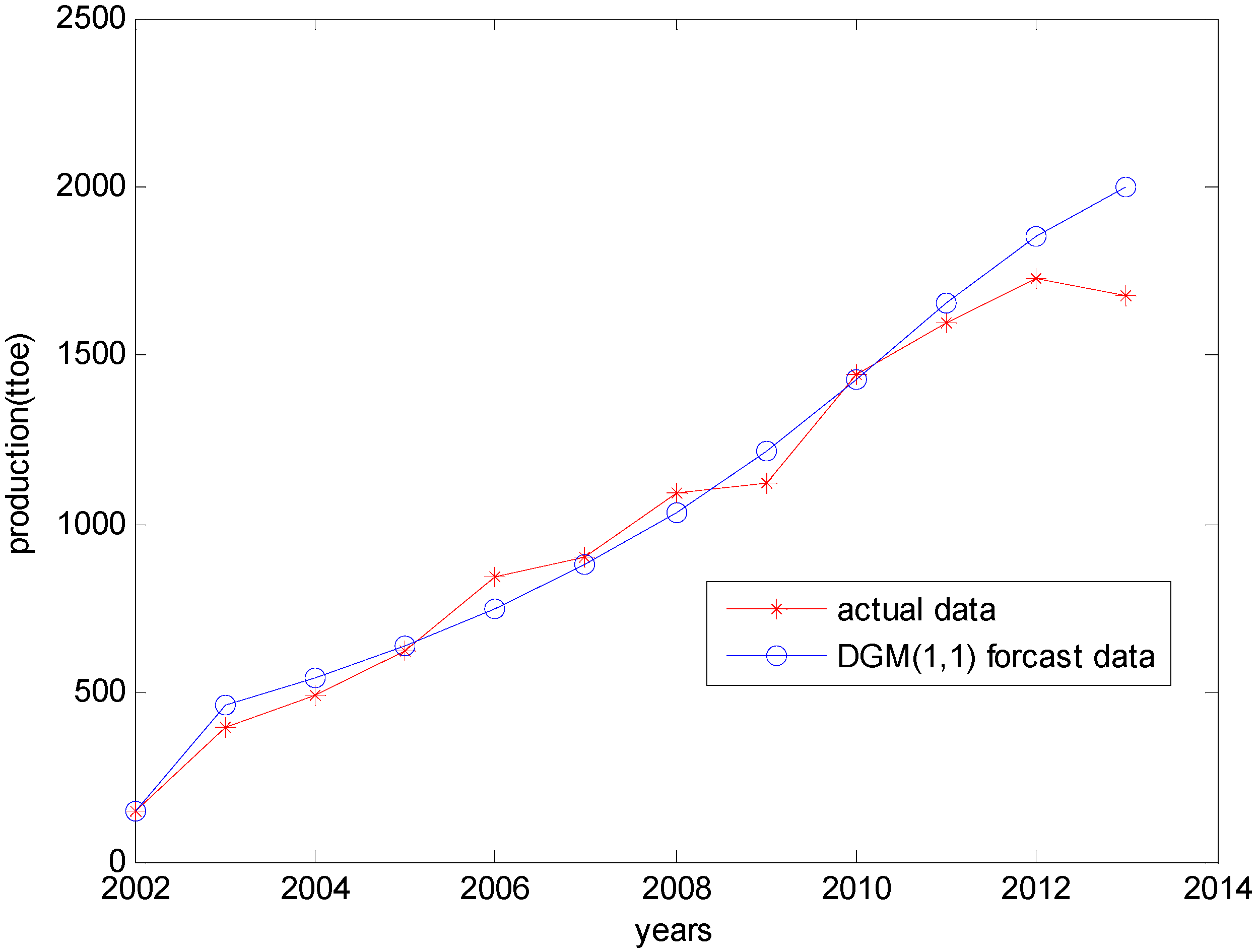
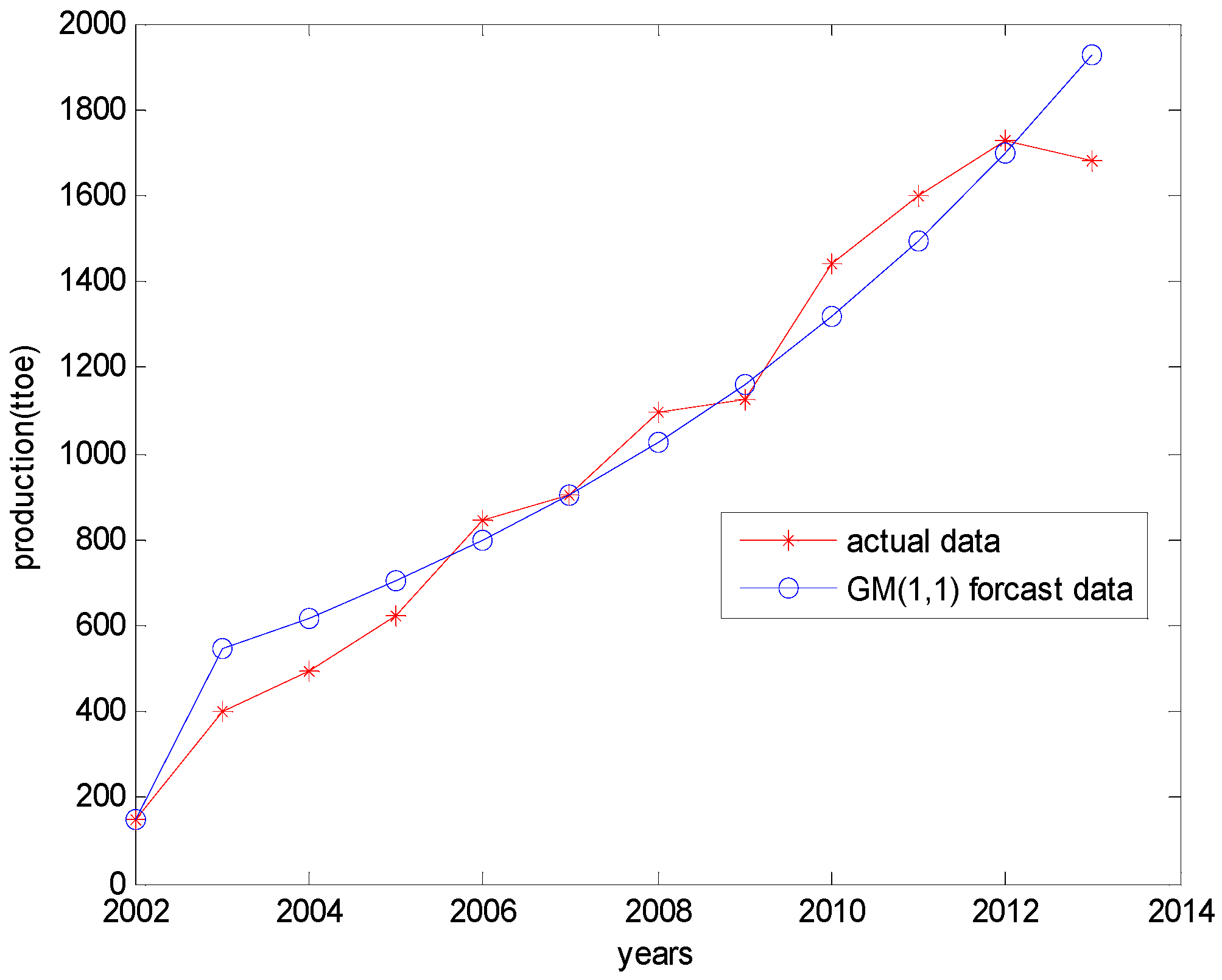
4.2. Results of the GM (1,1) Model

First, we apply the biofuel production data for 2002 to 2013 to the traditional GM (1,1) model and compare the analog output with the actual production. The results are shown in Table 2. The normal GM (1,1) forecast model equation calculated using Matlab software is as follows:

$$y_{(t+1)}=2607.8{\text{e}}^{0.18453t}-2290.8$$

(14)

Table 2. Forecast data using the grey model GM (1,1).

Years	Raw Data	GM (1,1) Data	Residual	Correctly Predicted Percentage
2002	148.00	148.00	0	100
2003	398.00	545.29	147.29	62.9925
2004	493.00	618.65	125.65	74.5132
2005	622.00	701.88	79.88	87.1576
2006	846.00	796.31	–49.69	94.1265
2007	901.00	903.44	2.44	99.7292
2008	1096.00	1025.00	–71.00	93.5219
2009	1124.00	1162.90	38.90	96.5392
2010	1441.00	1319.30	–121.70	91.5545
2011	1597.00	1496.80	–100.20	93.7257
2012	1729.00	1698.20	–30.80	98.2186
2013	1680.00	1926.70	246.7	85.3155

Table 2. Forecast data using the grey model GM (1,1).

Years	Raw Data	GM (1,1) Data	Residual	Correctly Predicted Percentage
2002	148.00	148.00	0	100
2003	398.00	545.29	147.29	62.9925
2004	493.00	618.65	125.65	74.5132
2005	622.00	701.88	79.88	87.1576
2006	846.00	796.31	–49.69	94.1265
2007	901.00	903.44	2.44	99.7292
2008	1096.00	1025.00	–71.00	93.5219
2009	1124.00	1162.90	38.90	96.5392
2010	1441.00	1319.30	–121.70	91.5545
2011	1597.00	1496.80	–100.20	93.7257
2012	1729.00	1698.20	–30.80	98.2186
2013	1680.00	1926.70	246.7	85.3155

In this model:

S₀ = 0.6745 × 110.2 = 74.3299

(15)

$$P=\left\{|{\mathrm{\Delta }}_k-\overline{\mathrm{\Delta }}|\right\}\le 0.6745s_1=\{0.00,62.77,41.13,-4.64,-34.83,-82.08,-13.52,-45.62,37.18,15.68,-53.72,162.18,\}=83.33\%$$

(16)

C = 0.2079

(17)

The simulation graphics are shown in Figure 3.

Figure 3. Prediction map of China’s biofuel production using the grey model GM (1,1) model.

Figure 3. Prediction map of China’s biofuel production using the grey model GM (1,1) model.

4.3. Results of the Dynamic Grey Prediction Model

We build the dynamic grey prediction model using the known original data sequence for biofuel production from 2002 to 2013. Thus:

$$X^{(0)}(148,398,493,622,846,901,1096,1124,1441,1597,1729,1680)$$

(18)

First, we use the dynamic grey prediction model to determine the best dimension and the best dimension prediction effect from multidimensional experiments. As seen from Table 3, the eighth dimension provides the lowest average relative error using the original statistical data fitting and considering the a posteriori ratios of the other seven dimensions. Thus, we choose the dimension with the highest precision, namely the eighth dimension of the dynamic grey prediction model, to estimate biofuel production.

Table 3. Dimensions and a posteriori error ratios using the discrete grey forecasting model DGM (1,1).

Dimension	4	5	6	7	8
C	0.2162	0.2394	0.2193	0.2209	0.2036
Dimension	9	10	11	12	-
C	0.2245	0.2493	0.2633	0.2079	-

Table 3. Dimensions and a posteriori error ratios using the discrete grey forecasting model DGM (1,1).

Dimension	4	5	6	7	8
C	0.2162	0.2394	0.2193	0.2209	0.2036
Dimension	9	10	11	12	-
C	0.2245	0.2493	0.2633	0.2079	-

Then, we compare the analog output with the actual production data and report the results (Table 4).

Table 4. Forecast data using the DGM (1,1) model.

Years	Raw Data	DGM (1,1) Data	Residual	Relative Error	Correctly Predicted Percentage
2002	148.00	148.00	0	0	100
2003	398.00	462.58	−64.58	−0.1396	86.0392
2004	493.00	543.28	−50.28	−0.0926	90.7451
2005	622.00	638.07	−16.07	−0.0252	97.4815
2006	846.00	749.39	96.61	0.1289	87.1082
2007	901.00	880.13	20.87	0.0237	97.6288
2008	1096.00	1033.70	62.30	0.0603	93.9731
2009	1124.00	1214.00	−90.00	−0.0741	92.5865
2010	1441.00	1425.80	15.20	0.0107	98.9339
2011	1597.00	1658.90	−61.90	−0.0373	96.2686
2012	1729.00	1852.00	−123.00	−0.0664	93.3585
2013	1680.00	2002.40	−322.40	−0.1610	83.8993

Table 4. Forecast data using the DGM (1,1) model.

Years	Raw Data	DGM (1,1) Data	Residual	Relative Error	Correctly Predicted Percentage
2002	148.00	148.00	0	0	100
2003	398.00	462.58	−64.58	−0.1396	86.0392
2004	493.00	543.28	−50.28	−0.0926	90.7451
2005	622.00	638.07	−16.07	−0.0252	97.4815
2006	846.00	749.39	96.61	0.1289	87.1082
2007	901.00	880.13	20.87	0.0237	97.6288
2008	1096.00	1033.70	62.30	0.0603	93.9731
2009	1124.00	1214.00	−90.00	−0.0741	92.5865
2010	1441.00	1425.80	15.20	0.0107	98.9339
2011	1597.00	1658.90	−61.90	−0.0373	96.2686
2012	1729.00	1852.00	−123.00	−0.0664	93.3585
2013	1680.00	2002.40	−322.40	−0.1610	83.8993

The accuracy is calculated below:

$$s_0=0.6745\times 98.519=66.451$$

(19)

$$P=\left\{|{\mathrm{\Delta }}_k-\overline{\mathrm{\Delta }}|\right\}\le 0.6745s_1=\{0.00,-12.35,-26.65,-60.86,19.68,-56.06,-14.63,13.07,-61.73,-15.03,46.07,245.47\}=91.6\%$$

(20)

C = 0.2036

(21)

The evaluated precision is high. Figure 4 shows the prediction map for biofuel production using the eighth dimension of the DGM (1,1) model.

Figure 4. Prediction map for biofuel production using the eighth dimension of the discrete grey forecasting model DGM (1,1).

Figure 4. Prediction map for biofuel production using the eighth dimension of the discrete grey forecasting model DGM (1,1).

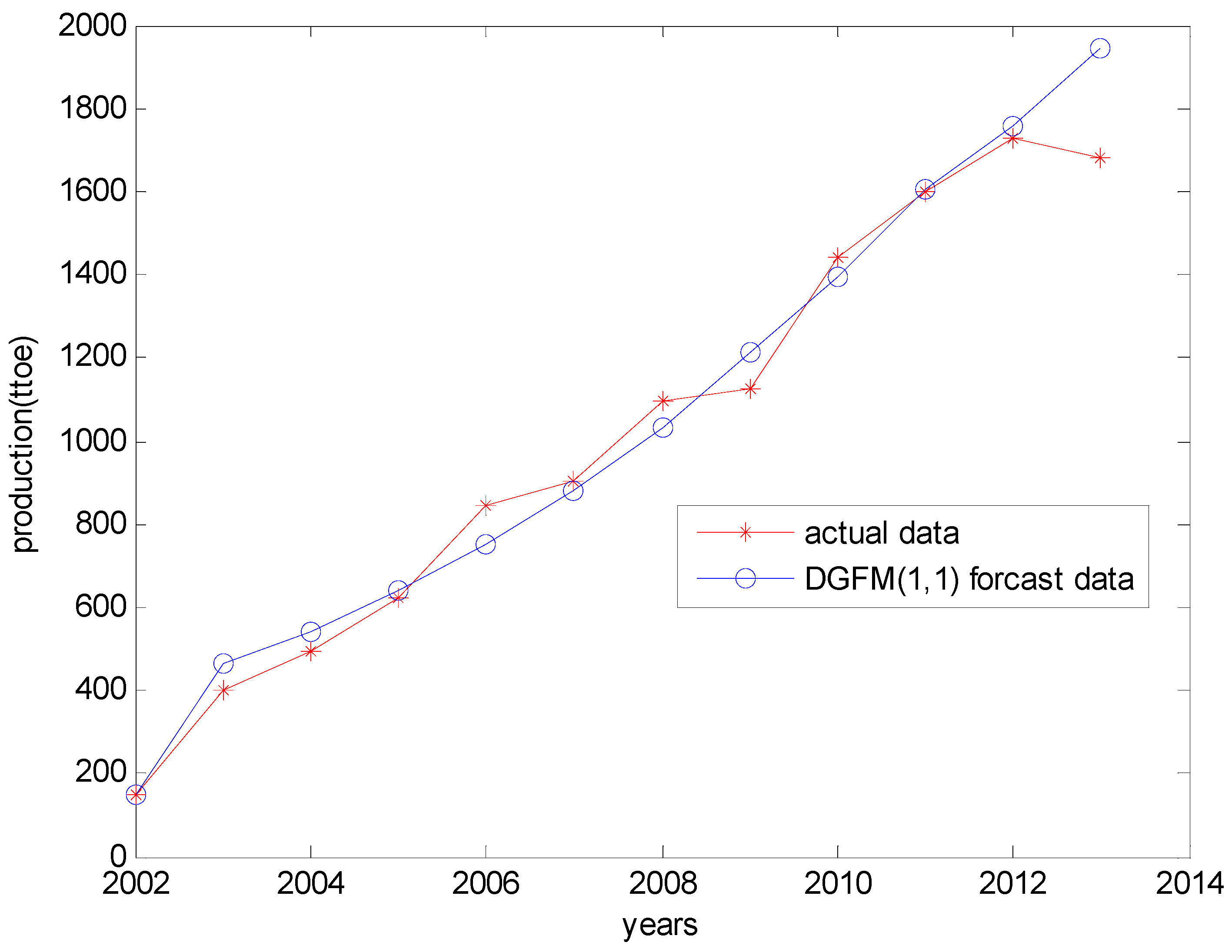
4.4. Results of the Dynamic Grey Fuzzy Markov Prediction Model

In this article, the biofuels production data column and its prediction residual error data columns are used as time series. Also, the experimental data columns are treated as homogeneous Markov chains with smooth transition probability, and accordingly, we can use the homogeneous Markov chain method to make our predictions.

In the first step, we use the data for 2010 to 2014 corrected by the Markov chain method to divide the information into different states, the target data being production from 2002 to 2009. Depending on our experience, the application of the Markov chain prediction method, and the contrasts in the relative errors of biofuel production, we refer to the following three states. Each state is defined as a fuzzy set, wherein all fuzzy states consist of a fuzzy space:

State 1: Underestimated state, where −20% ≤ relative error ≤ −5%. Table 4 shows that the data for 2003, 2004, and 2009 refer to this state.

State 2: Accurate assessment state, where −5% ≤ relative error ≤ 5%. Table 4 shows that the data for 2002, 2005, and 2007 refer to this state.

State 3: Overestimate state, 5% ≤ relative error ≤ 20%. According to Table 4, 2006 and 2008 refer to this state.

Each membership function of each fuzzy set is built using the triangle method, as seen below:

$$u_1(x)\{\begin{array}{cc}1\hfill & -20\%\le x\le -12.5\%\\ -8x\hfill & -12.5\%\le x\le 0\\ 0\hfill & \text{others}\end{array}$$

(22)

$$u_2(x)\{\begin{array}{cc}8x+1\hfill & -12.5\%\le x\le 0\\ 1-8x\hfill & 0\le x\le 12.5\%\\ 0\hfill & \text{others}\end{array}$$

(23)

$$u_3(x)\{\begin{array}{cc}8x\hfill & 0\le x\le 12.5\%\\ 1\hfill & 12.5\%\le x\le 20\%\\ 0\hfill & \text{others}\end{array}$$

(24)

We calculate each data point for the state vectors using the fuzzy membership function. This helps us categorize the data in terms of the state they belong to according to the principle of maximum membership (Table 5).

From Table 5, we arrive at the following one-step transition probability matrix for China’s biofuel production for the years 2002 to 2009:

$${{\displaystyle P}}^{(1)}=\left[\begin{array}{lll}1/2& 1/2& 0\\ 1/3& 0& 2/3\\ 1/2& 1/2& 0\end{array}\right]$$

(25)

According to the Markov chain prediction model $A^{(n)}=A^{(0)}{P}^{(n)}$, $A^{(n)}$ is a state probability vector of time n, and $A^{(0)}$ is a state probability vector of the initial moment. Thus, we calculate the fuzzy vector as its state with −7.414%, which is the relative error in 2009 (0.594, 0.406, 0). Thus, $A^{(0)}$ = (0.594, 0.406, 0).

Table 5. Categorizing China’s yearly biofuel production data into states according to the DGM (1,1) model (2002 to 2009).

Years	Raw Data	DGM (1,1) Data	Residual	Relative Error	State
2002	148.00	148.00	0	0	2
2003	398.00	462.58	−64.58	−0.1396	1
2004	493.00	543.28	−50.28	−0.0926	1
2005	622.00	638.07	−16.07	−0.0252	2
2006	846.00	749.39	96.61	0.1289	3
2007	901.00	880.13	20.87	0.0237	2
2008	1096.00	1033.70	62.30	0.0603	3
2009	1124.00	1214.00	−90.00	−0.0741	1

Table 5. Categorizing China’s yearly biofuel production data into states according to the DGM (1,1) model (2002 to 2009).

Years	Raw Data	DGM (1,1) Data	Residual	Relative Error	State
2002	148.00	148.00	0	0	2
2003	398.00	462.58	−64.58	−0.1396	1
2004	493.00	543.28	−50.28	−0.0926	1
2005	622.00	638.07	−16.07	−0.0252	2
2006	846.00	749.39	96.61	0.1289	3
2007	901.00	880.13	20.87	0.0237	2
2008	1096.00	1033.70	62.30	0.0603	3
2009	1124.00	1214.00	−90.00	−0.0741	1

Next, we conduct additional calculations to arrive at the prediction state vector for 2010 to 2013 (see Table 6).

Table 6. Prediction state vectors for 2010 to 2013.

State	2010	2011	2012	2013
1	0.4383	0.4475	0.4429	0.4452
2	0.3150	0.3425	0.3287	0.3356
3	0.2002	0.2100	0.2283	0.2192

Table 6. Prediction state vectors for 2010 to 2013.

State	2010	2011	2012	2013
1	0.4383	0.4475	0.4429	0.4452
2	0.3150	0.3425	0.3287	0.3356
3	0.2002	0.2100	0.2283	0.2192

Based on the above analysis, we continue making improvements via the Markov chain model using the results of grey dynamic prediction model. The improved results are shown in Table 7.

Table 7. Improved results with the Markov chain model.

Years	DGM (1,1) Data	Improved Result	Upper Limit	Lower Limit	Mid Value	Probability
2010	1425.80	1400.13	1226.19	1368.77	1297.48	0.44
	1425.80	-	1368.77	1482.83	1425.80	0.32
	1425.80	-	1482.83	1625.41	1554.12	0.25
2011	1658.90	1623.44	1426.65	1592.54	1509.60	0.45
	1658.90	-	1592.54	1725.26	1658.90	0.34
	1658.90	-	1725.26	1891.15	1808.20	0.21
2012	1852.00	1816.05	1592.72	1777.92	1685.32	0.44
	1852.00	-	1777.92	1926.08	1852.00	0.33
	1852.00	-	1926.08	2111.28	2018.68	0.23
2013	2002.40	1861.67	1722.06	1922.30	1822.18	0.45
	2002.40	-	1922.30	2082.50	2002.40	0.34
	2002.40	-	2082.50	2282.74	2182.62	0.22

Table 7. Improved results with the Markov chain model.

Years	DGM (1,1) Data	Improved Result	Upper Limit	Lower Limit	Mid Value	Probability
2010	1425.80	1400.13	1226.19	1368.77	1297.48	0.44
	1425.80	-	1368.77	1482.83	1425.80	0.32
	1425.80	-	1482.83	1625.41	1554.12	0.25
2011	1658.90	1623.44	1426.65	1592.54	1509.60	0.45
	1658.90	-	1592.54	1725.26	1658.90	0.34
	1658.90	-	1725.26	1891.15	1808.20	0.21
2012	1852.00	1816.05	1592.72	1777.92	1685.32	0.44
	1852.00	-	1777.92	1926.08	1852.00	0.33
	1852.00	-	1926.08	2111.28	2018.68	0.23
2013	2002.40	1861.67	1722.06	1922.30	1822.18	0.45
	2002.40	-	1922.30	2082.50	2002.40	0.34
	2002.40	-	2082.50	2282.74	2182.62	0.22

Table 8 shows the forecast data for China’s biofuel production from 2002 to 2013 using the DGFM (1,1) model.

Table 8. Forecast data using the dynamic grey fuzzy Markov DGFM (1,1) model (2002 to 2013).

Years	Raw Data	DGFM (1,1) Data	Residual	Relative Error
2002	148.00	148	0	0.0000
2003	398.00	462.58	−64.58	−0.1396
2004	493.00	543.28	−50.28	−0.0926
2005	622.00	638.07	−16.07	−0.0252
2006	846.00	749.39	96.61	0.1289
2007	901.00	880.13	20.87	0.0237
2008	1096.00	1033.7	62.3	0.0603
2009	1124.00	1214	−90	−0.0741
2010	1441.00	1400.13	40.87	0.0292
2011	1597.00	1623.44	−26.44	−0.0163
2012	1729.00	1816.05	−87.05	−0.0479
2013	1680.00	1861.67	−181.67	−0.0976

Table 8. Forecast data using the dynamic grey fuzzy Markov DGFM (1,1) model (2002 to 2013).

Years	Raw Data	DGFM (1,1) Data	Residual	Relative Error
2002	148.00	148	0	0.0000
2003	398.00	462.58	−64.58	−0.1396
2004	493.00	543.28	−50.28	−0.0926
2005	622.00	638.07	−16.07	−0.0252
2006	846.00	749.39	96.61	0.1289
2007	901.00	880.13	20.87	0.0237
2008	1096.00	1033.7	62.3	0.0603
2009	1124.00	1214	−90	−0.0741
2010	1441.00	1400.13	40.87	0.0292
2011	1597.00	1623.44	−26.44	−0.0163
2012	1729.00	1816.05	−87.05	−0.0479
2013	1680.00	1861.67	−181.67	−0.0976

In this model:

$$s_0=0.6745\times 76.50=51.59$$

(26)

$$P=\left\{|{\mathrm{\Delta }}_k-\overline{\mathrm{\Delta }}|\right\}\le 0.6745s_1=\{0.00,3.18,-11.12,-45.33,35.21,-40.53,0.90,28.60,-20.52,-34.95,25.65,120.28\}=91.6\%$$

(27)

C = 0.1443

(28)

The precision is high, as seen in Figure 5.

Figure 5. Prediction map for biofuel production using the dynamic grey fuzzy Markov DGFM (1,1) prediction model.

Figure 5. Prediction map for biofuel production using the dynamic grey fuzzy Markov DGFM (1,1) prediction model.

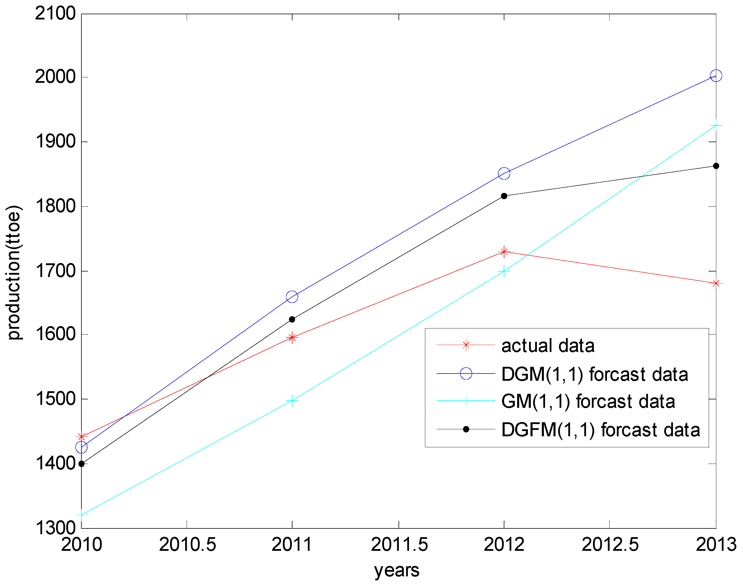
5. Comparison of the Three Methods

5.1. Comparison in Terms of Prediction Data

The results in Table 9 clearly indicate that the DGFM (1,1) model provides the closest fit to the actual data compared to the other two methods. Moreover, the DGFM (1,1) curve shown in Figure 6 is a better fit than the traditional GM (1,1) curve.

Table 9. Comparison of the three models with the actual data.

Years	Raw Data	GM (1,1)	DGM (1,1)	DGFM (1,1)
2010	1441.00	1319.30	1425.80	1400.13
2011	1597.00	1496.80	1658.90	1623.44
2012	1729.00	1698.20	1852.00	1816.05
2013	1680.00	1926.70	2002.40	1861.67

Table 9. Comparison of the three models with the actual data.

Years	Raw Data	GM (1,1)	DGM (1,1)	DGFM (1,1)
2010	1441.00	1319.30	1425.80	1400.13
2011	1597.00	1496.80	1658.90	1623.44
2012	1729.00	1698.20	1852.00	1816.05
2013	1680.00	1926.70	2002.40	1861.67

Figure 6. Comparison map of the three models and actual data.

Figure 6. Comparison map of the three models and actual data.

5.2. Comparison in Terms of Prediction Accuracy

Prediction accuracies are usually compared using the following three indicators: correctly predicted percentage, C value, and P value. Table 10 clearly shows that the DGFM (1,1) model outperforms the other models in terms of all three indicators; the DGFM (1,1) model has the lowest prediction error and the highest prediction accuracy.

Table 10. Comparison of the three models in terms of prediction accuracy.

Prediction Accuracies	GM (1,1)	DGM (1,1)	DGFM (1,1)
Correctly predicted percentage	92.20%	93.11%	94.91%
C-value	0.2079	0.2036	0.1443
p-value	83.30%	91.60%	91.60%

Table 10. Comparison of the three models in terms of prediction accuracy.

Prediction Accuracies	GM (1,1)	DGM (1,1)	DGFM (1,1)
Correctly predicted percentage	92.20%	93.11%	94.91%
C-value	0.2079	0.2036	0.1443
p-value	83.30%	91.60%	91.60%

Thus, the comparisons of the forecast values and prediction accuracy prove that the DGFM (1,1) model is the best in terms of both applicability and feasibility. Next, we use this model to forecast China’s biofuel production from 2015 to 2020.

6. Forecasting China’s Biofuel Production from 2015 to 2020 Using the DGFM (1,1) Model

6.1. Forecasting Process

Table 11 and Table 12 present the results of the forecast using the DGM (1,1) model and the results of the Markov process with DGM (1,1) prediction data respectively.

Table 11. Forecast of China’s biofuel production for 2015 to 2020 using the DGM (1,1) model.

Years	Forcasting Data	Years	Forcasting Data
2015	2203.40	2018	2835.80
2016	2413.10	2019	3115.70
2017	2595.90	2020	3436.10

Table 11. Forecast of China’s biofuel production for 2015 to 2020 using the DGM (1,1) model.

Years	Forcasting Data	Years	Forcasting Data
2015	2203.40	2018	2835.80
2016	2413.10	2019	3115.70
2017	2595.90	2020	3436.10

Table 12. Results of the Markov process with DGM (1,1) prediction data.

Years	Raw Data	DGM Data	Relative Error	State
2002	148.00	148.00	0.0000	2
2003	398.00	462.58	−0.1396	1
2004	493.00	543.28	−0.0926	1
2005	622.00	638.07	−0.0252	2
2006	846.00	749.39	0.1289	3
2007	901.00	880.13	0.0237	2
2008	1096.00	1033.70	0.0603	3
2009	1124.00	1214.00	−0.0741	1
2010	1441.00	1425.80	0.0107	2
2011	1597.00	1658.90	−0.0373	2
2012	1729.00	1852.00	−0.0664	1
2013	1680.00	2002.40	−0.1610	1

Table 12. Results of the Markov process with DGM (1,1) prediction data.

Years	Raw Data	DGM Data	Relative Error	State
2002	148.00	148.00	0.0000	2
2003	398.00	462.58	−0.1396	1
2004	493.00	543.28	−0.0926	1
2005	622.00	638.07	−0.0252	2
2006	846.00	749.39	0.1289	3
2007	901.00	880.13	0.0237	2
2008	1096.00	1033.70	0.0603	3
2009	1124.00	1214.00	−0.0741	1
2010	1441.00	1425.80	0.0107	2
2011	1597.00	1658.90	−0.0373	2
2012	1729.00	1852.00	−0.0664	1
2013	1680.00	2002.40	−0.1610	1

$${{\displaystyle P}}^{(1)}=\left[\begin{array}{lll}1/2& 1/2& 0\\ 1/3& 0& 2/3\\ 1/2& 1/2& 0\end{array}\right]A^{\left(0\right)}=(1,0,0)$$

(29)

The modified results are as seen in Table 13.

Table 13. Modified forecast of China’s biofuel production for 2015 to 2020 using the DGFM (1,1) model.

Years	Forcasting Data	Years	Forcasting Data
2015	2153.11	2018	2771.07
2016	2358.02	2019	3044.58
2017	2536.65	2020	3357.67

Table 13. Modified forecast of China’s biofuel production for 2015 to 2020 using the DGFM (1,1) model.

Years	Forcasting Data	Years	Forcasting Data
2015	2153.11	2018	2771.07
2016	2358.02	2019	3044.58
2017	2536.65	2020	3357.67

6.2. Analysis of the Results

Independent reports predict that by 2020 biofuels could account for 15% of the transportation energy consumption in China, with transport biofuels substituting 10% of conventional fuels. However, our forecast results for China’s biofuel production in the next five years using the grey dynamic fuzzy Markov prediction model show that between 2015 and 2020, China’s biofuel production will reach 2153.107, 2358.021, 2536.649, 2771.073, 3044.584, and 3357.671 ttoe, values which are well below the long-term development goal set for the year 2020 (i.e., 10,000 ttoe). That is, at its current development speed and given the present framework in the sector, biofuel production in China will be unable to achieve, and in fact, fall far short of, the national renewable energy plan target.

7. Conclusions

We used two kinds of conventional forecasting models, the GM (1,1) model and the grey dynamic fuzzy Markov prediction model, to forecast biofuel production in China for 2010 to 2013. Our results show that:

(1)

The grey dynamic fuzzy Markov prediction model can blend in new information in a timely and effective manner. Simultaneously, it can discard outdated information, that is, information declines caused by time lapses. Moreover, compared to the conventional model, the results of the grey dynamic fuzzy Markov prediction model closely mirror the actual data.

(2)

The grey dynamic fuzzy Markov prediction model is based on the conventional GM (1,1) prediction model. The proposed model is simple and easy to understand. It has strong applicability and shows high precision as a linear prediction model. Thus, it has important practical significance, as shown in this study, for biofuel production prediction.

Our forecast for biofuel production indicates that China will be unable to achieve its goal for 2020. The presence of state subsidies is likely to ensure that while the first generation of biofuels will gradually reduce, it will be hard to develop second-generation biofuel production technology within such a short time. There will be added pressure on increasing biofuel production in the future. However, appropriate raw materials, technology, and efficiency, especially the acquisition of and transformation technology improvements for second-generation biofuel raw materials, are necessary for breakthroughs. Additional enabling policy efforts are also needed. Otherwise, China will find it difficult to realize the development of alternative energy via biofuel production.

References

1. Annual Energy Outlook 2014; U.S. Energy Information Administration (EIA): Washington, DC, USA, 2014.
2. Domestic and International Oil and Gas Industry Development Report 2014; China National Petroleum Corporation (CNPC) Research Institute of Economics and Technology: Beijing, China, 2014. (In Chinese)
3. Odgaard, O.; Delman, J. China’s energy security and its challenges towards 2035. Energy Policy 2014, 71, 107–117. [Google Scholar] [CrossRef]
4. Research on China’s Medium and Long Term Energy Development Strategy; State Council Development Research Center: Beijing, China, 2011. (In Chinese)
5. Doku, A.; Di Falco, S. Biofuels in developing countries: Are comparative advantages enough? Energy Policy 2012, 44, 101–117. [Google Scholar] [CrossRef]
6. Charles, M.B.; Ryan, R.; Ryan, N.; Oloruntoba, R. Public policy and biofuels: The way forward? Energy Policy 2007, 35, 5737–5746. [Google Scholar] [CrossRef]
7. Wiesenthal, T.; Leduc, G.; Christidis, P.; Schade, B.; Pelkmans, L.; Govaerts, L.; Georgopoulos, P. Biofuel support policies in Europe: Lessons learnt for the long way ahead. Renew. Sustain. Energy Rev. 2009, 13, 789–800. [Google Scholar] [CrossRef]
8. Gregg, J.S.; Andres, R.J.; Marland, G. China: Emissions pattern of the world Leader in CO2 emissions from fossil fuel consumption and cement production. Geophys. Res. Lett. 2008, 35. [Google Scholar] [CrossRef]
9. Zhou, A.; Thomson, E. The development of biofuels in Asia. Appl. Energy 2009, 86, S11–S20. [Google Scholar] [CrossRef]
10. Environmental Protection Bureau (EPB). Available online: http://tech.sina.com.cn/d/2014-10-31/14329750274.shtml (accessed 31 October 2014). (In Chinese)
11. Wang, C.; Cai, W.J.; Lu, X.D.; Chen, J.N. CO2 mitigation scenarios in China’s road transport sector. Energy Convers. Manag. 2007, 48, 2110–2118. [Google Scholar] [CrossRef]
12. China’s Medium-Term and Long-Term Plan for Renewable Energy Development; National Development and Reform Commission: Beijing, China, 2007. (In Chinese)
13. Chang, S.Y.; Zhao, L.L.; Govinda, R.T.; Zhang, X.L. Biofuels development in China: Technology options and policies needed to meet the 2020 target. Energy Policy 2012, 51, 64–79. [Google Scholar] [CrossRef]
14. Qiu, H.G.; Huang, J.K.; Keyzer, M. Biofuel development, food security and the use of marginal land in China. J. Environ. Qual. 2011, 40, 1058–1067. [Google Scholar] [CrossRef] [PubMed]
15. Tian, Y.S.; Zhao, L.X.; Meng, H.B.; Sun, L.Y.; Yan, J.Y. Estimation of un-used land potential for biofuels development in (the) People’s Republic of China. Appl. Energy 2009, 86, S77–S85. [Google Scholar] [CrossRef]
16. Wu, Y.M. Research on Fiscal Policy Support for Fuel Ethanol Industry in China Using CGE Model. Ph.D. Thesis, University of Geosciences, Beijing, China, 2014. [Google Scholar]
17. Amirnekooei, K.; Ardehali, M.M.; Sadri, A. Integrated resource planning for Iran: Development of reference energy system, forecast, and long-term energy-environment plan. Energy 2012, 46, 374–385. [Google Scholar] [CrossRef]
18. Bennett, C.J.; Stewart, R.A.; Lu, J.W. Forecasting low voltage distribution network demand profiles using a pattern recognition based expert system. Energy 2014, 67, 200–212. [Google Scholar]
19. Tunckaya, Y.; Koklukaya, E. Comparative prediction analysis of 600 MWe coal-fired power plant production rate using statistical and neural-based models. J. Energy Inst. 2015, 88, 11–18. [Google Scholar] [CrossRef]
20. Carpinone, A.; Giorgio, M.; Langella, R.; Testa, A. Markov chain modeling for very-short-term wind power forecasting. Electr. Power Syst. Res. 2015, 122, 152–158. [Google Scholar] [CrossRef]
21. Urasawa, S. Real-time GDP forecasting for Japan: A dynamic factor model approach. J. Jpn. Int. Econ. 2014, 34, 116–134. [Google Scholar] [CrossRef]
22. Deng, J.L. Basis of Gray Theory; Huazhong University of Science and Technology Press: Wuhan, China, 1987. (In Chinese) [Google Scholar]
23. Deng, J.L. Introduction to grey system theory. J. Grey Syst. 1989, 1, 1–24. [Google Scholar]
24. Liu, S.F.; Deng, J.L. The range suitable for GM(1,1). Syst. Eng. Theory Pract. 2000, 20, 121–124. [Google Scholar]
25. Xiong, P.P.; Dang, Y.G.; Yao, T.X.; Wang, Z.X. Optimal modeling and forecasting of the energy consumption and production in China. Energy 2014, 77, 623–634. [Google Scholar] [CrossRef]
26. Hamzacebi, C.; Es, H.A. Forecasting the annual electricity consumption of Turkey using an optimized grey model. Energy 2014, 70, 165–171. [Google Scholar] [CrossRef]
27. Soldo, B. Forecasting natural gas consumption. Appl. Energy 2012, 92, 26–37. [Google Scholar] [CrossRef]
28. Wu, L.F.; Liu, S.F.; Liu, D.L.; Fang, Z.G.; Xu, H.Y. Modeling and forecasting CO2 emissions in the BRICS (Brazil, Russia, India, China, and South Africa) countries using a novel multi-variable grey model. Energy 2015, 79, 489–495. [Google Scholar] [CrossRef]
29. Wang, J.Z.; Dong, Y.; Wu, J.; Mu, R.; Jiang, H. Coal production forecast and low carbon policies in China. Energy Policy 2011, 39, 5970–5979. [Google Scholar] [CrossRef]
30. Lin, C.T.; Yang, S.Y. Forecast of the output value of Taiwan’s opto-electronics industry using the Grey forecasting model. Technol. Forecast. Soc. Change 2003, 70, 177–186. [Google Scholar] [CrossRef]
31. Truong, D.Q.; Ahn, K.K. Wave prediction based on a modified grey model MGM(1,1) for real time control of wave energy converters in irregular waves. Renew. Energy 2012, 43, 242–255. [Google Scholar] [CrossRef]
32. Liu, X.Y.; Peng, H.Q.; Bai, Y.; Zhu, Y.J.; Liao, L.L. Tourism Flows Prediction based on an Improved Grey GM(1,1) model. Soc. Behav. Sci. 2014, 138, 767–775. [Google Scholar] [CrossRef]
33. Xie, N.M.; Liu, S.F. Discrete grey forecasting model and its optimization. Appl. Math. Model. 2009, 33, 1173–1186. [Google Scholar] [CrossRef]
34. Tien, T.L. A new grey prediction model FGM(1, 1). Math. Comput. Model. 2009, 49, 1416–1426. [Google Scholar] [CrossRef]
35. Li, D.C.; Yeh, C.W.; Chang, C.J. An improved grey-based approach for early manufacturing data forecasting. Comput. Ind. Eng. 2009, 57, 1161–1167. [Google Scholar] [CrossRef]
36. Ou, S.L. Forecasting agricultural output with an improved grey forecasting model based on the genetic algorithm. Comput. Electron. Agric. 2012, 85, 33–39. [Google Scholar] [CrossRef]
37. Evans, M. An alternative approach to estimating the parameters of a generalized Grey Verhulst model: An application to steel intensity of use in the UK. Expert Syst. Appl. 2014, 41, 1236–1244. [Google Scholar] [CrossRef]
38. Oztaysi, B. A decision model for information technology selection using AHP integrated Topsis-Grey: The case of content management systems. Knowl. Based Syst. 2014, 70, 44–54. [Google Scholar] [CrossRef]
39. Bahrami, S.; Hooshmand, R.; Parastegari, M. Short term electric load forecasting by wavelet transform and grey model improved by PSO (particle swarm optimization) algorithm. Energy 2014, 72, 434–442. [Google Scholar] [CrossRef]
40. Wang, H.Y.; Ma, F. A study of information renewal GM(1,1) model for predicting urban medium and long-term water demand. Eng. J. Wuhan Univ. 2004, 37, 32–36. [Google Scholar]
41. Zhou, Z.L.; Yin, C.W. Application of Grey metabolic Model in the prediction of the Cotton Output in China. Asian Agric. Res. 2011, 3, 1–6. [Google Scholar]
42. BP Statistical Review of World Energy 2014. Available online: http://www.bp.com/zh_cn/china/reports-and-publications/bp_2014.html (accessed on 1 June 2014).