Article

An Experimental Study on the Effects ofWinglets on the Wake and Performance of a ModelWind Turbine

1
Department of Mechanical Science and Engineering, University of Illinois, Urbana, IL 61801, USA
2
Department of Civil and Environmental Engineering, University of Illinois, Urbana, IL 61801, USA
*
Author to whom correspondence should be addressed.
Energies 2015, 8(10), 11955-11972; https://doi.org/10.3390/en81011955
Submission received: 25 August 2015 / Revised: 25 September 2015 / Accepted: 3 October 2015 / Published: 21 October 2015
(This article belongs to the Special Issue Wind Turbine 2015)

Abstract

:
Wind tunnel experiments were performed to investigate the effects of downstream-facing winglets on the wake dynamics, power and thrust of a model wind turbine. Two similar turbines with and without winglets were operated under the same conditions. Results show an increase in the power and thrust coefficients of 8.2% and 15.0% for the wingletted case. A simple theoretical treatment of a two-turbine system suggests a possible positive tradeoff between increasing power and thrust coefficients at a wind farm scale. The higher thrust coefficient created a region of enhanced mean shear and turbulence in the outer portion of the wake. The winglets did not significantly change the tip-vortex strength, but higher levels of turbulence in the far wake decreased the tip-vortex strength. Because of the increased mean shear in the wingletted turbine’s wake, the Reynolds stresses were higher, potentially leading to a higher energy flux downstream.

1. Introduction

By restricting the spanwise velocity over a wing or turbine blade, the downwash created by wingtip vortices can be diminished, decreasing the induced drag [1] and leading to more favorable aerodynamics. The tip-vortex system induces velocities perpendicular to the freestream direction. According to Prandtl’s lifting line theory, the inviscid lift force is perpendicular to the direction of the flow, so an additional drag force is created in the freestream direction by the tip-vortex induced velocities. Therefore, the restriction of the wingtip vortex is of significant interest, and winglets have proven to be an effective tool in the reduction of induced drag. According to Kroo [2], the addition of a winglet to a wing contributes a reduction in tip loss effects of ∼45% as much as would be gained from increasing the blade span by the same length as the winglet height.
Because wind turbine blade length may be constrained by transportation considerations [3], winglets may also be an attractive addition for such blades. Johansen and Sørensen [4] numerically investigated several winglet designs, and identified adjustable parameters including the winglet height, radius of curvature, and various winglet-associated angles. The winglets investigated in that study increased the power coefficient by 0.6% to 1.4% for upstream-facing winglets, with a corresponding increase in thrust coefficient of 1.0% to 1.6%; whereas a downstream-facing winglet increased the power coefficient by up to 1.7%, with an increase in thrust coefficient of 1.8%. The increases in power and thrust coefficients were found to be dependent on the tip-speed ratio (λ), and became negative at low speeds for several designs. Imamura et al. [5] investigated the effects of winglets on a wind turbine rotor with a vortex lattice method, and altered the dihedral angle (defined as the upward angle that the winglet makes from horizontal) from 80 to a 0 (equivalent to a radial extension). Their results suggested that a winglet positioned close to 90 from the plane of the rotor was most effective at increasing power coefficient, and showed that the decrease in downwash is also highest for these winglets. Promisingly, their results also suggested that the increase in bending moment from winglets was comparable to radial extension, meaning no additional structural loads need to be considered in the design. Further numerical investigation by Chattot [6] looked at the effect on power production of several wingtip alterations on wind turbines, and showed promise for winglets as well as dihedral bending of the blade. While an increase in power coefficient is possible, it is important to note that the Lanchester–Betz–Joukowsky limit [7] still holds. A theoretical investigation by Gauna and Johansen [8] used the concept of an actuator cap, similar to the actuator disk in the momentum theory, with the addition of a cylinder representing winglets. The theory demonstrated that the Lanchester–Betz–Joukowsky limit holds for a turbine with winglets, and suggests that power increases come from a reduction in tip losses, rather than a downwind shift in wake vorticity as previously suggested by Van Bussel [9].
Although it has been established in the literature that a turbine with winglets has the potential to increase power coefficient, the effect of the altered wake in the context of turbulent wind farm dynamics is unclear. The alteration of the wake structure may have a significant effect on total wind farm power, as turbulent stresses are the dominant pathway to wake re-energization [10]. This process can be triggered by the breakdown of the tip vortices according to Lignarolo et al. [11], who observed a significant increase in Reynolds stress concentration after vortex spiral breakdown due to the mutual-inductance mode instability identified by Widnall [12]. It has also been noted that the helical tip vortex structure is unconditionally unstable in the far wake, as identified by Okulov and Sørensen [13]. A change in tip-vortex circulation may be expected to alter the onset of this instability, as the linear stability analysis of an infinite row of point vortices predicts that the perturbation growth rate is proportional to the vortex strength [14].
This paper focuses on the study of wind turbine wakes behind turbines with and without winglets experiencing an incoming turbulent boundary layer in a laboratory wind tunnel. We compare performance statistics with previous computational works, and investigate the effects of winglets on wake dynamics and the subsequent wake re-energization. Experimental details are given in Section 2, significant results are presented in Section 3, important results are discussed in Section 4, and concluding thoughts are provided in Section 5.

2. Experimental Setup

Two horizontal-axis model wind turbines of equal rotor diameter were placed and operated in an Eiffel-type wind tunnel. One turbine has a standard rotor design, whereas downwind-facing winglets were added to the blades of the other model, as these were shown in the literature to be the most effective at increasing the power coefficient. The turbines and their wakes were tested in a boundary layer developed over a smooth wall that reached ∼80% of the turbine hub height. Details of the experimental setup are described as follows.

2.1. Model Turbines

Two horizontal-axis model wind turbines of d T = 0.12 m rotor diameter, P 0 1 W rated power, and z h u b = 0.125 m hub height were built, based on a reference model turbine from Sandia National Labs [15,16]. The blades and nacelle were fabricated at the University of Illinois Rapid-Prototyping Lab using an Objet Eden 350 machine and were made of PolyJet Vero material. The basic geometry of the blades is provided in Table 1. A Precision Microdrives 112-001 Micro Core 12 mm DC Motor is used as a loading system to control the angular velocity, Ω, which was set to approximately 295 rad·s - 1 , giving a tip-speed ratio of λ = Ω R / U h u b = 5 . 4 , where R = 0.06 m is the rotor radius and U h u b = 11.5 m·s - 1 is the incoming mean velocity at hub height. The tower was made of a 4 mm diameter threaded steel rod. Refer to Tobin et al. [17] for similar setup. The winglets are made by extending and bending the blade’s tip with a 4 mm radius of curvature and 4 mm out-of-plane height, giving a winglet length 6 . 7 % of the turbine radius, while maintaining the rotor radius as projected in the axial direction. It should be noted that this length is larger than the 1%–4% radius winglets tested by Johansen and Sørensen [4]; the larger size of our winglets was constrained by the 3D printing process. A schematic of the rotor with and without winglets is shown in Figure 1. Turbine power output was acquired with a Measurement Computing USB-1608HS datalogger and instantaneous voltage was measured directly from the terminals of the DC generator. Power was then inferred from instantaneous voltage and the resistance across the terminals of the datalogger. Voltage was sampled at a rate of 1 kHz for a duration of 120 s.
Table 1. Basic geometry of the model wind turbine blades normalized by the rotor radius: c is the chord length, α is the angle with respect to the rotor plane.
ParameterNormalized radial location ( r / R )
0 . 2 0 . 3 0 . 4 0 . 5 0 . 6 0 . 7 0 . 8 0 . 9 0 . 95
c / R 0 . 275 0 . 248 0 . 215 0 . 181 0 . 156 0 . 136 0 . 119 0 . 100 0 . 088
α ( ) 31 . 8 23 . 9 17 . 7 12 . 8 9 . 4 7 . 5 6 . 0 4 . 6 3 . 9
Figure 1. Schematic of the miniature turbine. (a) schematic of rotor, nacelle and loading system; (b) base miniature wind turbine; (c) standard and wingletted rotor details.
Energies 08 11955 g001

2.2. Image Collection and Processing

The 2D Velocity field measurements were acquired with a planar particle image velocimetry (PIV) system from TSI. The flow was seeded with 1 μm olive oil droplets generated by several Laskin nozzles placed upwind of the wind tunnel inlet. A 250 mJ/pulse double-pulsed laser (Quantel) was used to illuminate the field of view (FOV) of an 11 MP (4000 × 2672 pixel) 12 bit frame-straddle CCD camera. The spanwise-normal laser sheet was 1 mm thick, and the FOV was 170 mm × 260 mm (streamwise by wall-normal). Measurements were performed for three regions in the wake of each turbine model: two adjacent regions extending from x / d T = 0.2 to 2.6 behind the rotor, and a region farther downstream, 4 x / d T 5.3. Figure 2 illustrates the general setup and the three FOV. The measurements in the three regions were obtained by keeping the PIV setup stationary and moving the turbines upwind. The interrogation area was near the end of the 6.1 m test section, and the turbines were moved a total of 0.45 m. Assuming Prandtl’s turbulent boundary layer depth growth δ ( x ) / x = 0 . 376 ( U x / ν ) - 1 / 5 [18], boundary layer depth would change from δ / δ 0 = 1 at the farthest upwind location of the turbines (where δ 0 = 0.100 m is the boundary layer depth at this location) to δ / δ 0 = 1.06 at the farthest downwind location. This difference is deemed adequately small for the purpose of this study. Five thousand image pairs were collected for each of the six cases (three regions for each of the two turbines) at a frequency of 1 Hz. For the boundary layer measurements, 1800 image pairs were used, with the same sampling rate. Image pairs were interrogated with a recursive cross-correlation method using Insight 4G software package from TSI. The final interrogation window was 16 × 16 pixels with 50% overlap, resulting in a final vector grid spacing Δ x = Δ z = 0 . 52 mm.
Figure 2. Schematic of the experimental setup for the standard and wingletted wind turbines including the three FOV.
Energies 08 11955 g002

2.3. Incoming Flow

The model wind turbines were tested in the wind tunnel of the University of Illinois at Urbana-Champaign’s Renewable Energy and Turbulent Environment Group (RETEG). The Eiffel-type wind tunnel has a test-section 0.914 m wide, 0.457 m high, and 6.1 m long and an adjustable ceiling calibrated to allow the boundary layer to grow in zero pressure gradient. More details on the facility can be found in Adrian et al. [19]. The incoming boundary layer was developed over a smooth wall and tripped at the beginning of the test section with a 5 mm diameter rod. At the location of the turbine, the turbulent boundary layer reaches ∼80% the height of the rotor hub. Above the height of the boundary layer there is a uniform, low turbulence flow (∼0.5% turbulence intensity). It should be noted that this boundary layer height is not typical for wind turbine operation; however, significant insights may still be gleaned from the experimental results, allowing for investigation in different flow regimes. The turbulent boundary layer had a shear velocity u τ = 0 . 404 m·s - 1 , roughness length z 0 = 0.24 mm, and δ 0 . 1 m at the location of the PIV setup. The freestream velocity was U = 11.5 m·s - 1 , giving a turbine rotor Reynolds number R e d = U d T / ν = 9.2 × 10 4 , which is in the limit where mean statistics in the wake are insensitive to Reynolds number [20]. The same planar particle image velocimetry setup used to quantify the wind turbine wake (Figure 2) was employed to characterize the incoming flow at the same location with no turbine. Figure 3 shows non-dimensional vertical profiles of the incoming flow including the streamwise velocity component U / U h u b , turbulence intensity σ u / U h u b and kinematic Reynolds stress - u w ¯ / u τ 2 . Figure 4 shows the approximate growth of the boundary layer over the region in which the turbine was operated.
Figure 3. Non-dimensional characteristics of the incoming boundary layer. (a) mean velocity profile U / U h u b ; (b) turbulence intensity σ u / U h u b ; (c) Reynolds stress - u w ¯ / u τ 2 . Horizontal dashed lines indicate the bottom and top tips of the turbine.
Energies 08 11955 g003
Figure 4. Visualization of boundary layer growth around the measurement location. Thick black line indicates Prandtl boundary layer depth. Horizontal dashed lines indicate the bottom and top tips of the turbine. Vertical lines indicate the locations where the turbine was placed. Green area is where PIV measurements were taken.
Energies 08 11955 g004

3. Results

3.1. Turbine Power and Thrust

The two turbines tested in this work were operated under identical flow conditions, as indicated in Section 2.3. In total 120,000 instantaneous measurements of power output were taken directly from the generator, and indicate that the turbine with winglets improved the power output of the standard turbine, with power coefficients C P = 2 P / ρ A U h u b 3 ∼0.119 and 0.110 respectively, i.e., an increase of 8.2%. The wingletted turbine also experienced an increase in the thrust coefficient, with C T = 0.52 over the base one, C T = 0.45; i.e., an increase of ∼15%. A simple method of estimating thrust coefficient is given in Equations (1) and (2), where T is the total thrust force, U w is the velocity in the wake of the turbine, U is the boundary layer velocity, and A is a plane of integration that captures the entirety of the wake deficit. However, velocity fields were only measured in the central plane. To account for this problem, the wake flow was estimated by subtracting the measured wake deficit (discussed in Section 3.3) at the appropriate radial locations from the measured boundary layer flow—where the top half of the rotor disk used the upper measured wake deficit, and the bottom half used the lower measured wake deficit. The calculated thrust values were constant (within 5%) with downstream distance.
T = ρ A U w ( r , θ ) ( U ( r , θ ) - U w ( r , θ ) d A
C T = 2 T / ( ρ U h u b 2 π / 4 d T 2 )

3.2. Formulation of a Theoretical Model

The increase in C P resultant from the addition of winglets must be weighed against the consequent increase in C T . Although an individual turbine will benefit from increased C P , higher wake deficits resultant from increased C T may reduce the power production of downwind turbines. While this compromise may be exceedingly complex in a real wind farm, a simple case may help illustrate the tradeoff. Here, we consider one wind turbine directly upwind of another, and use the simplified wake model proposed by Jensen [21] to estimate total power output of the system. Note that the Jensen model is only a crude estimate, and other, more accurate, wake models may be used in its place (see Bastankhah and Porté-Agel [22] for a discussion on the subject of wake modeling). The Jensen wake model assumes a top-hat distribution for the wake deficit, and uses the principle of mass conservation in the linearly expanding wake. The velocity downstream of a turbine is given in Equation (3), where U u p is the undisturbed upstream velocity, U d o w n is the velocity downstream of the first turbine, κ is the wake expansion coefficient, and x is separation distance between the two turbines. Typical values of C T = 0.8 and κ = 0.05 suggested by Barthelmie et al. [23] for an offshore wind farm will be used.
U d o w n ( x ) = U u p 1 - 1 - 1 - C T ( 1 + 2 κ x / d T ) 2
The upwind turbine faces a velocity of U u p and the downwind turbine faces a velocity of U d o w n . Then, supposing the addition of winglets to the rotor increased the power coefficient by a given percentage, an acceptable increase in thrust coefficient can be estimated by considering the combined power output of the two turbines. The upwind turbine will be expected to produce a power output of P 1 = C P ρ π d T 2 U u p 3 / 4 , and the downwind one will produce P 2 = C P ρ π d T 2 U d o w n 3 / 4 . By setting P 1 / C P equal to unity, the total power output of the system is given in Equation (4).
P t o t = C P + C P 1 - 1 - 1 - C T ( 1 + 2 κ x / d T ) 2 3
Taking the effects of the winglets into account by increasing C P and C T , the maximum allowable increase in C T that will keep the combined power output unchanged can be calculated for a given increase in C P . Note that while the initial value of the C T changes the results, the initial value of the C P does not. 
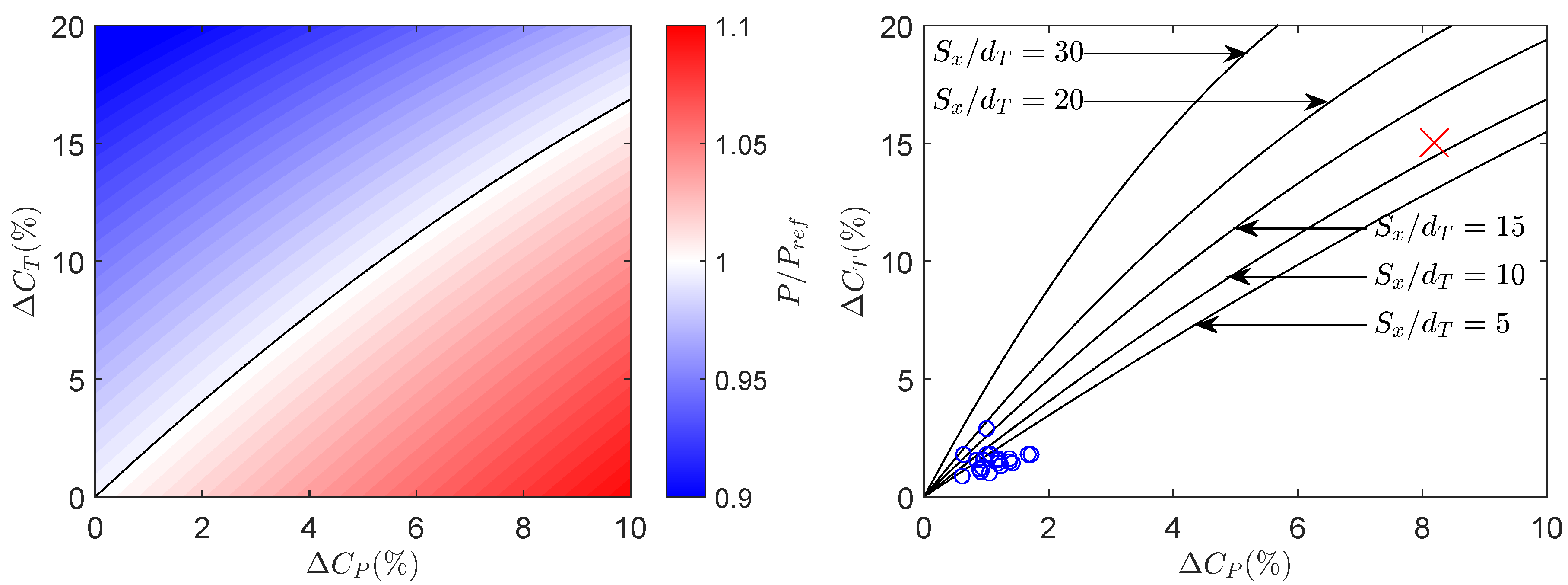
Figure 5 shows the results of this analysis, where Δ C P is the increase in C P from adding winglets, Δ C T is the increase in C T , P is the combined power of the two wingletted turbines, and P r e f is the power output of the two turbines with reference values of C P and C T . The left figure uses an inter-turbine spacing of 10 rotor diameters and shows the combined power output, where red areas have a higher output than the base case, and blue areas have a lower output, and the black line shows the border between the two. The right figure shows the break-even curve for several inter-turbine spacings.
Figure 5. Illustration of maximum allowable increase in C T for a given increase in C P . Left: combined power output for given increase in C P and C T , normalized by the reference power, where inter-turbine spacing is 10 rotor diameters. Right: break-even lines for several inter-turbine spacings. Red crosses come from this experiment. Blue circles are from Johansen and Sørensen.
Energies 08 11955 g005

3.3. Wake Characteristics

Due to the ∼15% increase in C T 
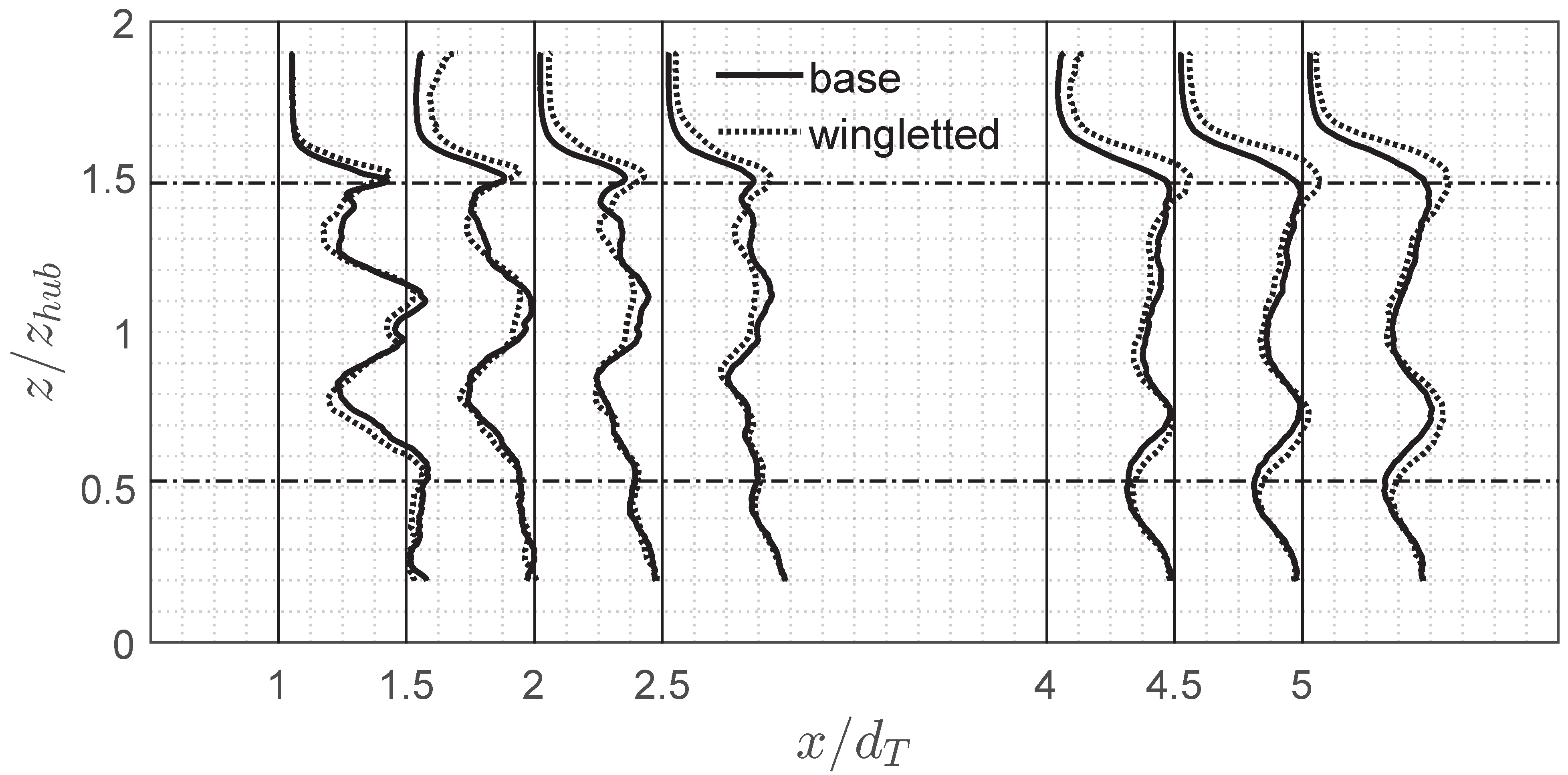
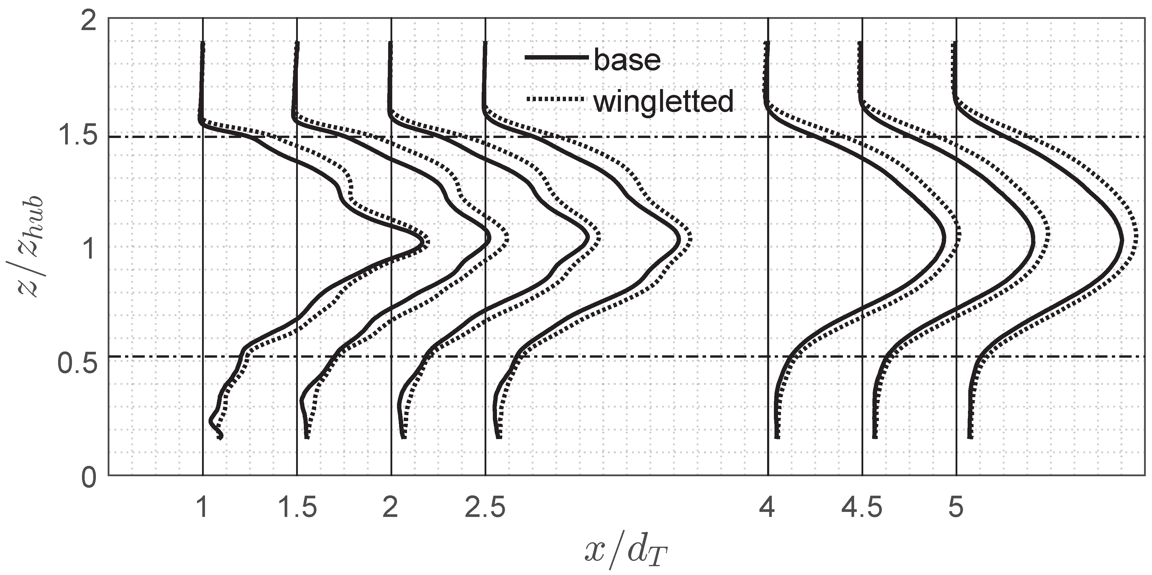
caused by the winglets, there is a non-negligible difference in the velocity defect profile in the near wake region, as illustrated in Figure 6. The difference is the greatest in the outer portions of the turbine wake, where the downwash-diminishing effect of the winglets is the highest. In the outer portions of the rotor, the difference in velocity defect is up to 10% of the mean incoming velocity. This is consistent with the results of Johansen and Sørensen [4], where the force distribution was increased in the outer 14% of the rotor. While the difference in velocity defect becomes less localized downstream by turbulent mixing, the total wake deficit that might be experienced by a downstream turbine stays consistently higher in the wingletted case. The average wake deficit, Δ U ( x ) ¯ 
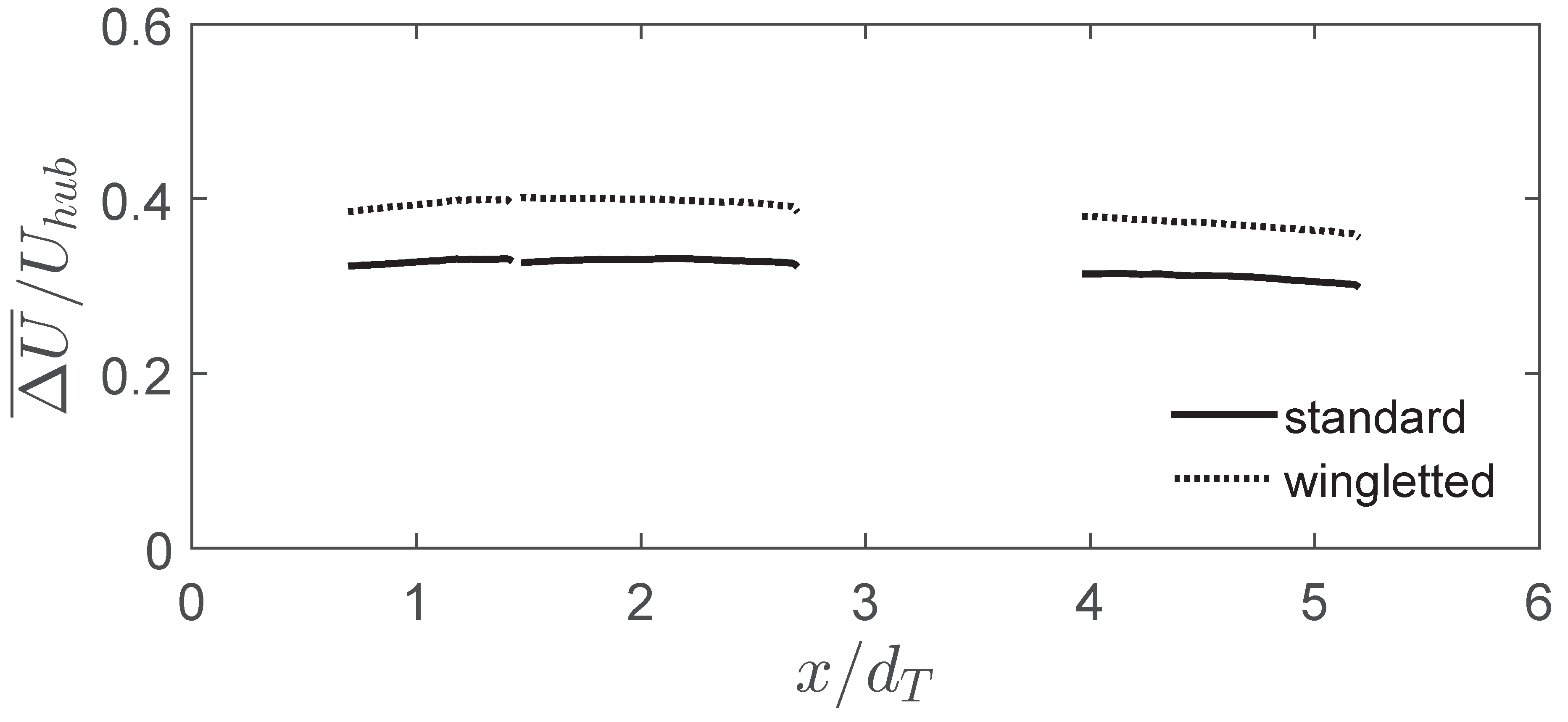
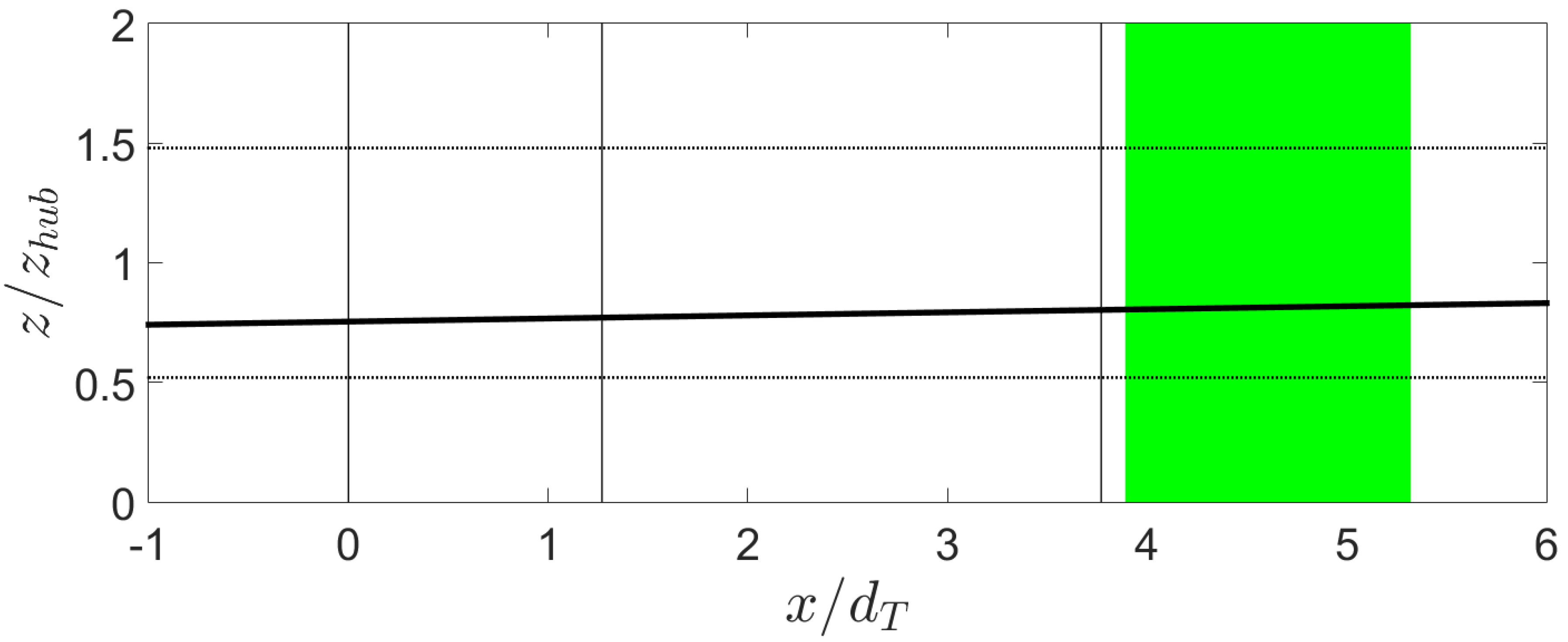
, was calculated with a solid of revolution concept in the same way as the thrust coefficient was, where the top and bottom measured wake profiles were assumed as the radial distribution over their respective half of the rotor area. Results for the standard and wingletted cases are given in Figure 7. The total wake deficit is higher by ∼6% of the hub height velocity in the wingletted case. The difference in average wake deficit does not change significantly with downstream distance.
Figure 6. Comparison of the mean wake deficit profiles, Δ U ( x , z ) = U i n c ( z ) - U ( x , z ) , at the central plane of the standard and wingletted turbine models at several downstream locations. Horizontal dash-dot lines indicate the location of the bottom and top tips of the turbine. Vertical solid lines indicate local zeros, and grid squares have a width of 0.1 × U h u b .
Energies 08 11955 g006
Figure 7. Non-dimensional average wake deficit Δ U ¯ / U h u b for the two turbine cases as a function of downstream distance.
Energies 08 11955 g007
In addition to larger velocity deficits, the wingletted turbine also exhibits slightly higher turbulence intensity in the third FOV (4 x / d T 5.3), which is illustrated in Figure 8. This is a result of the higher mean shear in the outer portion of the rotor of the wingletted turbine wake due to the increased thrust force, as the generation of turbulent kinetic energy G = - 1 2 u i u j ¯ ( u j x i + u i x j ¯ ) .
Figure 8. Comparison of the standard deviation of velocity profiles at the central plane of the standard and wingletted turbine models at several downstream locations. Horizontal dash-dot lines indicate the location of the bottom and top tips of the turbine. Vertical solid lines indicate local zeros, and grid squares have a width of 0.025 × U h u b .
Energies 08 11955 g008
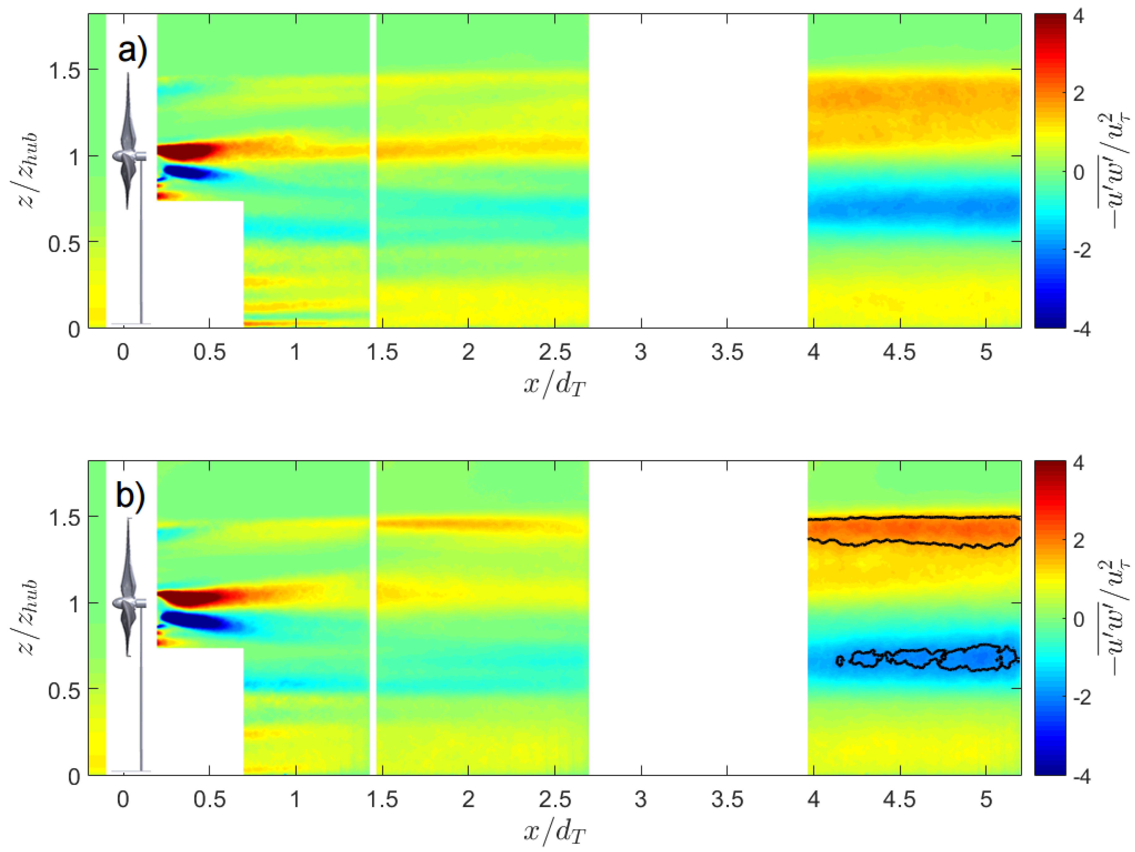
The Reynolds stresses are significantly altered by the addition of winglets to the turbine. In the third FOV at x / d T = 5 , the streamwise-vertical component of the Reynolds stress is 10% higher for the wingletted turbine in the outer top part of the wake, shown in Figure 9. The black lines in Figure 9b highlight the region of greater Reynolds stress, and are contours of the maximum levels from the base case. To quantify the extent to which the flow has reached an equilibrium state, we apply Prandtl’s mixing length theory for jets and wakes. In the mixing length theory, the Reynolds stress can be modeled as in Equation (5),
- u w ¯ = b Δ ( x ) u ¯ 0 ( x ) u z
where Δ ( x ) is the wake width, u ¯ 0 ( x ) is the maximum velocity defect, and b is a constant, reported as b 6 . 2 × 10 - 3 by Davidson [24] for a round jet when Δ is defined such that the wake deficit Δ / 2 away from the centerline is 10% the centerline value. The wake width is estimated from the PIV measurements, and the centerline wake deficit is taken locally as u ¯ 0 ( x ) = m a x z ( U i n c ( z ) - U ( x , z ) ) , where U i n c ( z ) is the velocity of the incoming boundary layer at height 
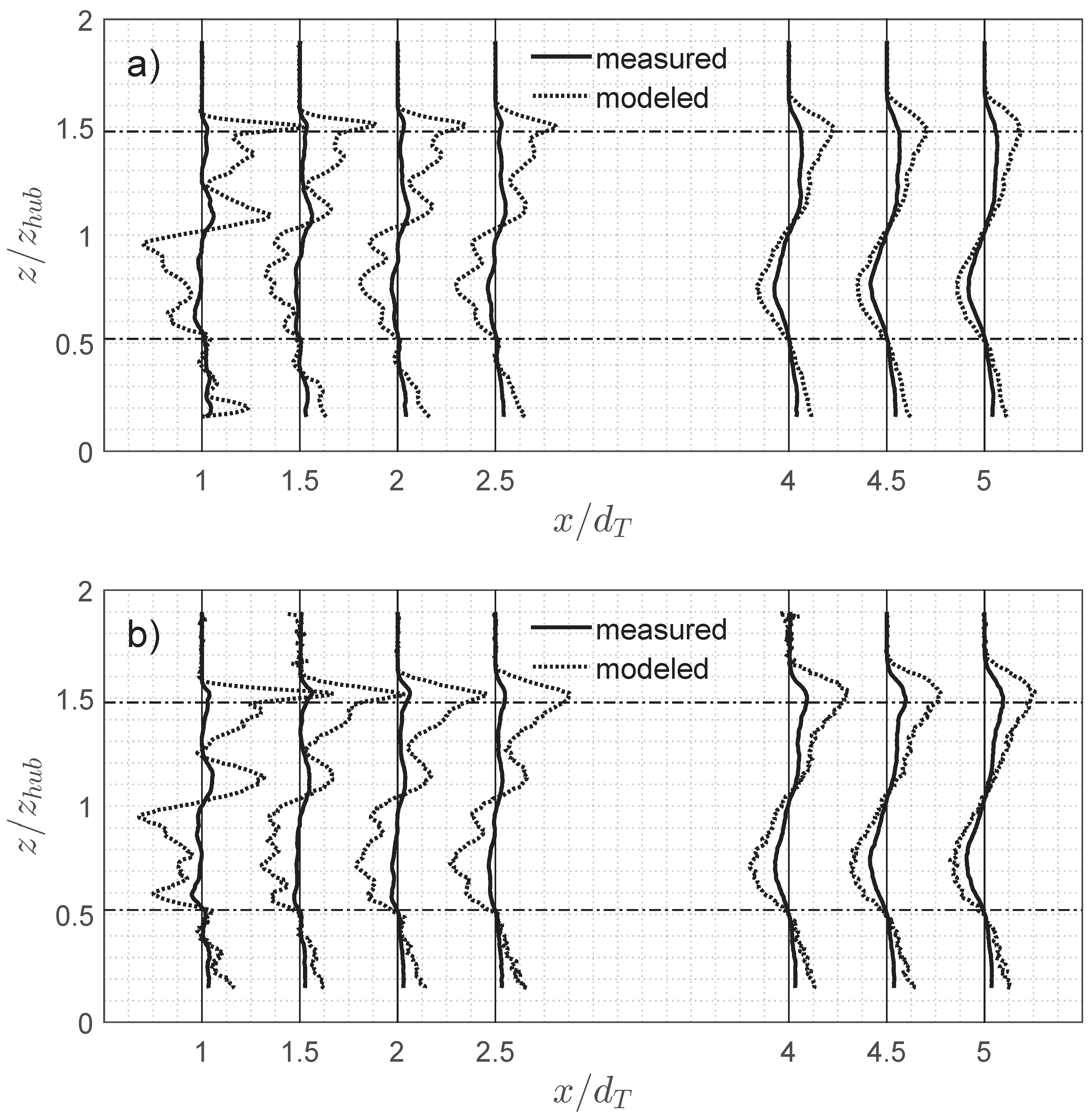
z. By comparing the measured and estimated distributions of - u w ¯ , as shown in Figure 10, a measure of the degree of self-similarity can be determined, since the measured Reynolds stress is expected to match the mixing length theory in a fully developed turbulent flow. The mismatch between them in a non-equilibrium flow is indicative of the further potential for the flow to attain a self-similar shape via turbulence production by mean shear. A root mean square (r.m.s.) error, ϵ r m s 
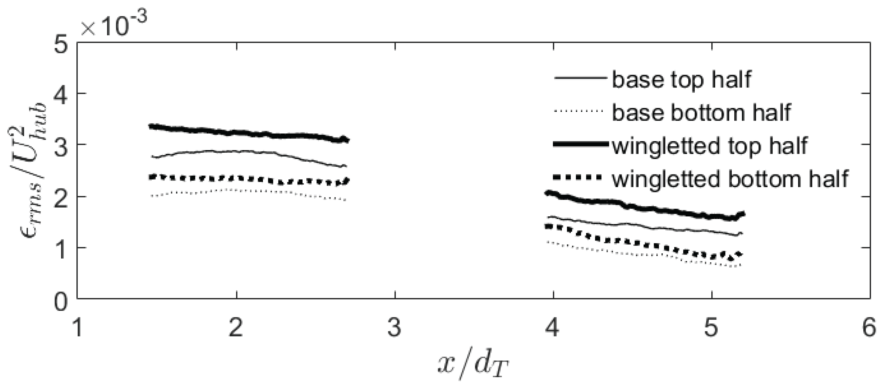
, of the mixing length model’s prediction is used as a quantitative means to compare the self-similarity between the two cases, because a fully self-similar flow will be most effectively spreading the momentum deficit due to the higher levels of turbulent shear stress. These r.m.s. values for both turbines, and for both the top and bottom parts of the wake, are illustrated in Figure 11. When calculating r.m.s. values for the top or bottom, points reaching from the hub to 1.4R were considered, so as to account for wake expansion (results from the first FOV are excluded due to the strong effect of the generator’s wake). Results indicate that the base turbine is closer to equilibrium than the wingletted one at all downstream locations, and that the lower, more turbulent portion of the wake is also closer to equilibrium. This is likely a result of the higher levels of shear in the wingletted wake that need to be diffused by the turbulence. It should be noted that the analysis above is rather simplified—the model of the Reynolds stress should be, in general, a function of the initial disturbance and radial position (see Johansson et al. [25] for an in-depth discussion of axisymmetric turbulent wakes). The results are not particularly sensitive to the value of b; changing the value by 50% in either direction changes the magnitudes of the r.m.s. errors, but not their rankings.
Figure 9. Reynolds stress distribution in the turbine wake: (a) standard rotor; (b) wingletted. Incoming Reynolds stress is shown upstream of the turbine. Areas in the third panel enclosed in black contours have values higher than the maxima in (a).
Energies 08 11955 g009
Figure 10. Comparison between measured kinematic Reynolds stress and the shear-based mixing length model. (a) Base turbine; (b) wingletted turbine. Horizontal dash-dot lines indicate the location of the bottom and top tips of the turbine. Vertical solid lines indicate local zeros, and grid squares have a width of 2 × 10 - 3 U h u b 2 .
Energies 08 11955 g010
Figure 11. Normalized root mean square error ( ϵ r m s ) of mixing length estimate with downstream distance.
Energies 08 11955 g011
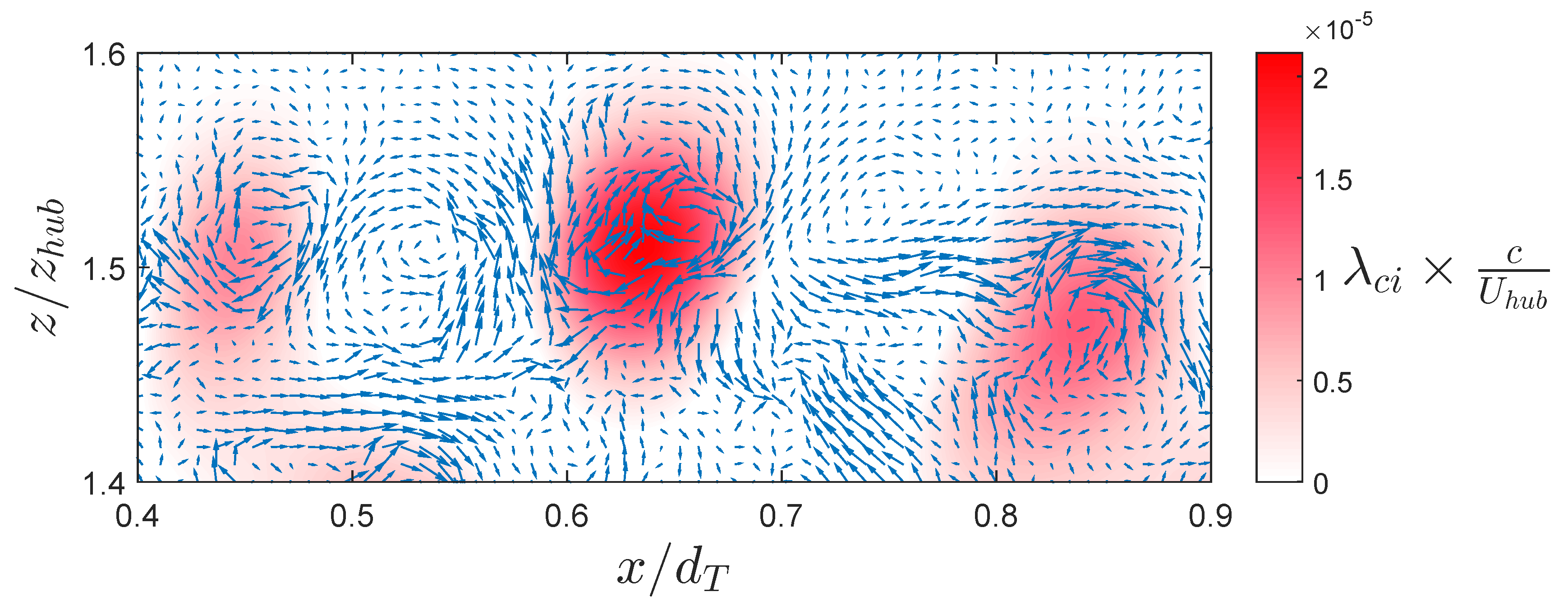
Further, the tip-vortex features were investigated by determining vortex strength as a function of downstream distance. The PIV velocity fields were conditioned using an LES decomposition with a filter width approximately the size of the tip vortex to eliminate small-scale structures, while the λ c i criterion of the filtered velocity field was used to identify tip vortices. For further information on the LES conditioning of velocity fields and identification of vortices, see Adrian et al. [26]. The quantity λ c i is the imaginary part of the complex conjugate eigenvalues of the velocity gradient tensor [27]. By calculating λ c i of the filtered velocity field, individual vortices are identified. A continuous (8-connected) region of non-zero λ c i was taken as a single tip vortex, with its core coincident with the maximum value of λ c i . An example λ c i field overlaid with instantaneous velocity vectors is shown in Figure 12. When a vortex core was identified, the instantaneous field was counted into an average that also had a core at that specific downstream location, giving phase-averaged results. Some tolerance was given for the z-location of the vortex core, but ∼90% were within one core radius of the average 
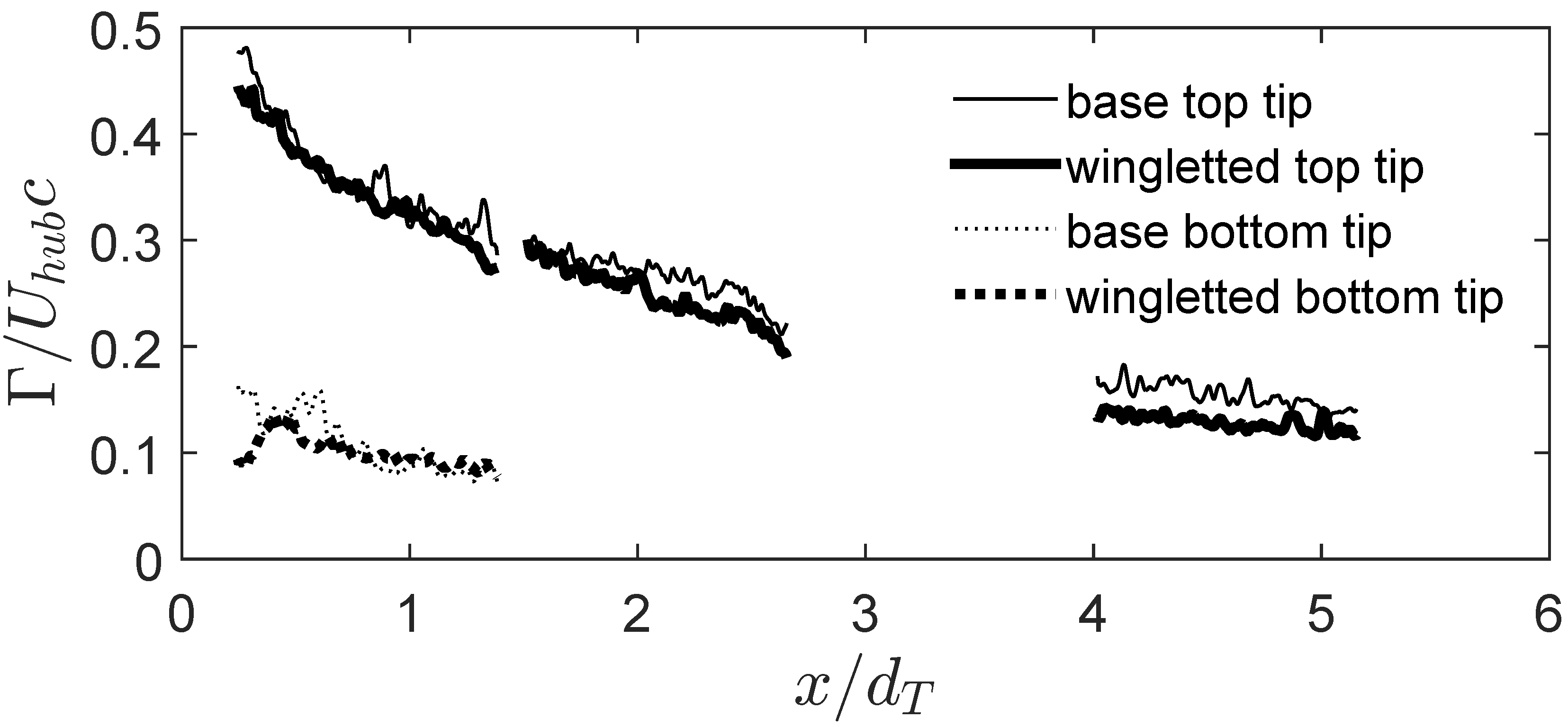
z-location. Between 50 and 125 fields were used for each streamwise location. This averaging allowed for the quantification of tip-vortex strength and the exclusion of turbulent vortices from the averaging farther downstream. The average non-dimensional vortex strength, where Γ is the vortex circulation and c is the average chord length, with downstream distance is shown in Figure 13 for the two turbine cases at the bottom and top tips. Circulation was measured with a closed path integral of the velocity field as defined in Equation (6) along a square circuit 7.25 mm on a side to coincide with the radial position of maximum tangential velocity. This is considered the characteristic circulation of a viscous vortex [28].
Γ = C u · d l = A ( × u ) · n ^ d S
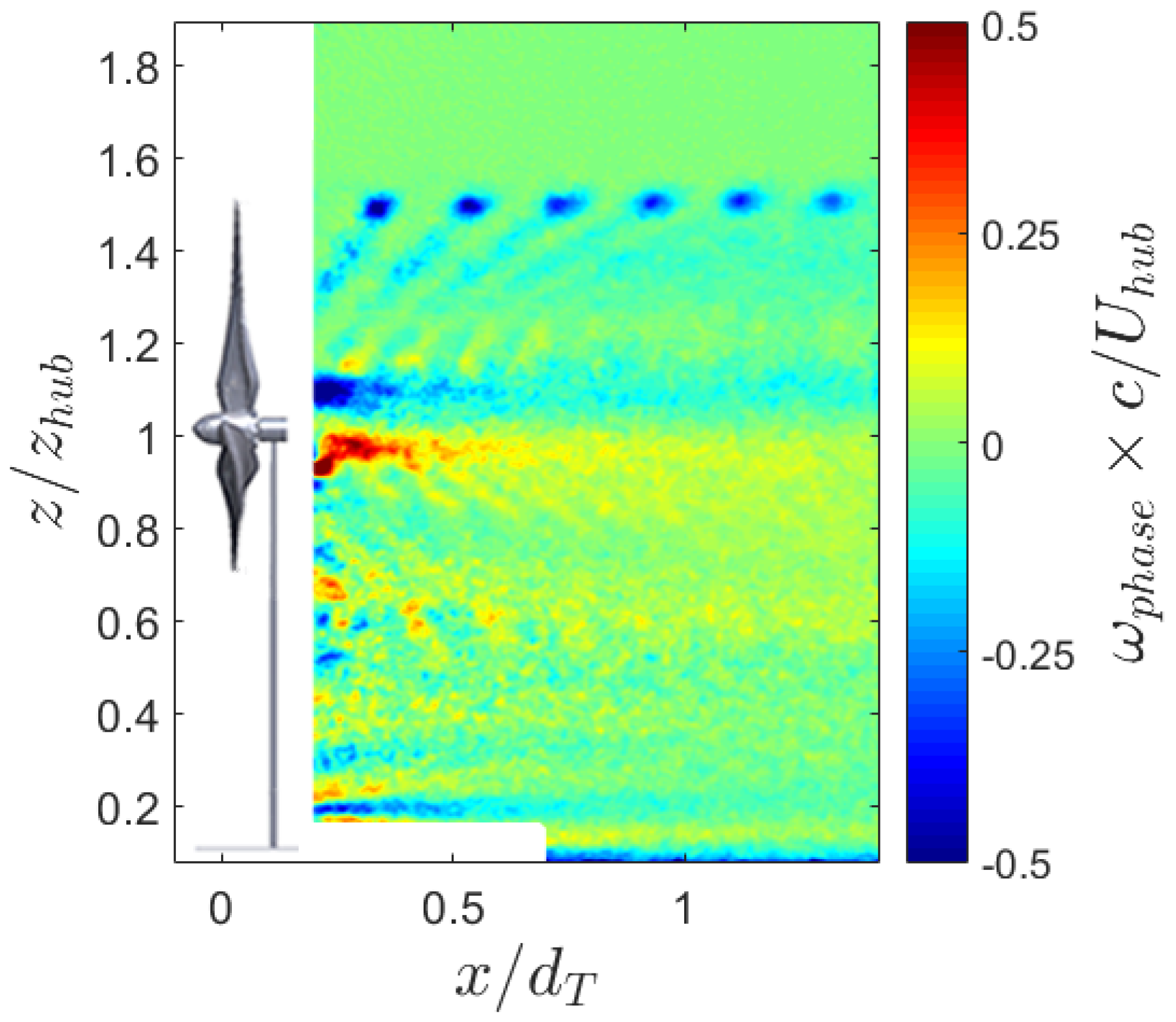
Example phase-average contours are given in Figure 14, clearly showing the tip-vortex structures and the footprint of the vortex sheet along the blades very near the turbine. The difference in tip-vortex strength measured in the upper half of the wake in the base and wingletted turbine cases becomes more pronounced farther downwind, where the base turbine has slightly stronger tip vortices, potentially as a result of the lower turbulence intensity. While the tip vortex may be predicted to be smaller from a wingletted airfoil, it is possible that the similar values observed in this study come from the fact that the area of integration for the circulation is larger on a side than the length of the winglet, thereby including some vorticity from the base of the wing as well as the body of the winglet. Also included in Figure 13 is the strength of vortices from the bottom tip. The lower values are likely a result of the vortex structure passing over the tower.
Figure 12. Instantaneous velocity field fluctuations overlaid on λ c i (red area) to illustrate the identification of tip vortices.
Energies 08 11955 g012
Figure 13. Average tip-vortex strength Γ as a function of the distance from the turbine for the standard and wingletted turbines.
Energies 08 11955 g013
Figure 14. Example phase-average vorticity contour ( ω p h a s e = × u p h a s e where u p h a s e is phase-average velocity) for the base turbine, normalized with blade chord length c and hub velocity U h u b .
Energies 08 11955 g014

4. Discussion

Results depicted in Figure 5 suggest that even for relatively low inter-turbine spacing, power losses due to an increase in C T can be offset by a relatively modest increase in C P . For a given inter-turbine spacing, as long as the Δ C P Δ C T coordinate is below the curves shown, there will be a total increase in power output.
The values of C P and C T found in this experiment are slightly above the line for a 10 rotor diameter spacing (shown in Figure 5 with a red cross). This inter-turbine spacing is fairly common in practice, although turbines are only directly upwind and downwind of each other occasionally. Increases in power and thrust were also published by Johansen and Sørensen [4] for their winglet designs; although results were dependent on the tip-speed ratio λ, the majority of their winglet-λ combinations (17 of 24) lie below the 5 rotor diameter spacing line (shown in Figure 5 as blue circles). Imamura et al. [5] also published the results of adding a winglet of length 10% the rotor radius, which led to an increase in C P of ∼20% and an increase in C T of ∼10%, though these were dependent on λ (results not depicted in Figure 5). It is unclear why these results outpaced the results of this work and of Johansen and Sørensen to such an extent, neither of which observed Δ C P ( % ) / Δ C T ( % ) > 1. Because the winglets in the current study represent an intermediate value between those of Johansen and Sørensen and those of Imamura et al., it is possible that longer winglets are more efficient at increasing power coefficient.
With the experimental results presented, it is possible to evaluate the predictive capability of the model derived in Section 3.2. Using the measurements of C T , C P , and the velocity field that a turbine placed 5 rotor diameters would experience in the two cases, and assuming a value of κ = 0.05 for a smooth wall (or an offshore wind farm [23]), the model predicts that two wingletted turbines will produce 3% more power than two base turbines. Again, using a solid of rotation concept to approximate the velocity faced by a downwind turbine, it is estimated from measurements that two wingletted turbines would produce ∼2% more power than two base turbines. This discrepancy may be explained by the fact that near-wake expansion is slowed because a full transition to turbulence has yet to occur. The results of the above analysis suggest that the effects on C T must be taken into account when considering wingletted turbines in a wind farm; however, it would seem reasonable that a wind farm can be designed such that the positive effects of winglets on C P outweighs the negative effects on C T .
In addition to having a favorable effect on a wind farm scale, the increase in power coefficient from the tested design also compared favorably when considering a single turbine. Because the height and radius of curvature of the winglet were both 4 mm, the equivalent additional blade length ( Δ L ) added to the rotor is Δ L / R 0 . 038 . If used to increase blade length radially, this would lead to an increase in rotor area (and correspondingly power output) of 7.8%. The addition of the winglets was, therefore, as effective as increasing rotor radius. This result contradicts the suggestion by Kroo [2] that a winglet is worth ∼45% of its height as additional span. However, results by Gauna and Johansen [8] have also shown that downstream-facing winglets can increase power coefficient nearly as well as radial extension, with near 100% effectiveness.

5. Concluding Remarks

The effects of winglets on a wind turbine with regards to wake dynamics and effects on wind farms are investigated. The rotor tested increased C P by 8.2% while increasing C T by 15%. A simple analysis on the effects of increasing both C P and C T with winglets in a 2-turbine system suggests that the winglet designs used in the current and one previous study may increase total wind farm power, but caution may need to be taken. The wake dynamics were also investigated; the primary characteristic effect of the winglets on the wake is identified as an increase in mean shear in the near wake, and a consequent increase in both turbulence intensity and kinematic Reynolds stress in the far wake. The wake of the wingletted turbine also exhibits higher levels of momentum deficit, which is not recovered over the streamwise distance interrogated despite the higher momentum flux from the Reynolds stresses. Turbulent properties of the wake approached equilibrium quicker in the bottom, more turbulent part of the wake, and also for the base turbine. Measurements of tip vortices indicate that winglets do not appreciably alter their strength except for downwind effects of higher turbulence destroying coherence, suggesting that aerodynamic improvements come from a downwind shift in the tip-vortex structure rather than diminishing its magnitude. Future efforts will focus on testing in deeper boundary layers, as well as performing multi-turbine experiments to further investigate the effects of winglets on wind farm power.

Acknowledgments

This material is based upon work supported by the National Science Foundation Graduate Research Fellowship Program under Grant Number DGE-1144245. This work was supported by the Department of Mechanical Science and Engineering, University of Illinois at Urbana-Champaign, as part of the start-up package of Leonardo P. Chamorro. The authors would like to acknowledge the efforts of Arpeet Kamdar and Karthik Ramaswamy in the preparation of the experiment and manuscript.

Author Contributions

Ali Hamed was responsible for the PIV setup. Nicolas Tobin processed and analyzed the data, and prepared the majority of the manuscript. All authors edited and commented on the manuscript.

Conflicts of Interest

The authors declare no conflict of interest.

References

  1. Maughmer, M.D. Design of winglets for high-performance sailplanes. J. Aircr. 2003, 40, 1099–1106. [Google Scholar] [CrossRef]
  2. Kroo, I. Drag due to lift: Concepts for prediction and reduction. Annu. Rev. Fluid Mech. 2001, 33, 587–617. [Google Scholar] [CrossRef]
  3. Cotrell, J.; Stehly, T.; Johnson, J.; Roberts, J.O.; Parker, Z.; Scott, G.; Heimiller, D. Analysis of Transportation and Logistics Challenges Affecting the Deployment of Larger Wind Turbines: Summary of Results; National Renewable Energy Laboratory: Bolder, CO, USA, 2014.
  4. Johansen, J.; Sørensen, N.N. Aerodynamic Investigation of Winglets on Wind Turbine Blades Using CFD; Technical Report “Risø-R-1543(EN)”; Risø National Laboratory: Roskilde, Denmark, 2006. [Google Scholar]
  5. Imamura, H.; Hasegawa, Y.; Kikuyama, K. Numerical analysis of the horizontal axis wind turbine with winglets. JSME Int. J. B-Fluid Therm. 1998, 41, 170–176. [Google Scholar] [CrossRef]
  6. Chattot, J.-J. Effects of blade tip modifications on wind turbine performance using vortex model. Comput. Fluids 2009, 38, 1405–1410. [Google Scholar] [CrossRef]
  7. Van Kuik, G.A.M. The Lanchester–Betz–Joukowsky limit. Wind Energy 2007, 10, 289–291. [Google Scholar] [CrossRef]
  8. Gauna, M.; Johansen, J. Determination of the maximum aerodynamic efficiency of wind turbine rotors with winglets. J. Phys. Conf. Ser. 2007, 75, 012006:1–012006:12. [Google Scholar] [CrossRef]
  9. Van Bussel, G.J.W. A momentum theory for winglets on horizontal axis wind turbine rotors and some comparison with experiments. In Proceedings of the Fourth International Energy Agency Symposium on the Aerodynamics of Wind Turbines, Rome, Italy, 19–20 November 1990.
  10. Cal, R.B.; Lebrón, J.; Castillo, L.; Kang, H.S.; Meneveau, C. Experimental study of the horizontally averaged flow structure in a model wind-turbine array boundary layer. Renew. Sust. Energy Rev. 2010, 2, 013106:1–013106:25. [Google Scholar] [CrossRef]
  11. Lignarolo, L.E.M.; Ragni, D.; Krishnaswami, C.; Chen, Q.; Simão Ferreira, C.J.; van Bussel, G.J.W. Experimental analysis of the wake of a horizontal-axis wind-turbine model. Renew. Energy 2014, 70, 31–46. [Google Scholar] [CrossRef]
  12. Widnall, S.E. The stability of a helical vortex filament. J. Fluid Mech. 1972, 54, 641–663. [Google Scholar] [CrossRef]
  13. Okulov, V.L.; Sørensen, J.N. Stability of Helical Tip Vortices in a Rotor Far Wake. J. Fluid Mech. 2007, 576, 1–25. [Google Scholar] [CrossRef]
  14. Aref, H. On the equilibrium and stability of a row of point vortices. J. Fluid Mech. 1995, 290, 167–181. [Google Scholar] [CrossRef]
  15. Shiu, H.; van Dam, C.P.; Johnson, E.; Barone, M.; Phillips, R.; Straka, W.; Fontaine, A.; Jonson, M. A design of a hydrofoil family for current-driven marine-hydrokinetic turbines. In Proceedings of the 20th International Conference on Nuclear Engineering and the American Society of Mechanical Engineers 2012 Power Conference, Anaheim, CA, USA, 30 July–3 August 2012; pp. 839–847.
  16. Johnson, E.; Fontaine, A.A.; Jonson, M.L.; Meyer, R.S.; Straka, W.A.; Young, S.; van Dam, C.P.; Shiu, H.; Barone, M. A 1:8.7 scale water tunnel test of an axial flow water turbine. In Proceedings of the 1st Marine Energy Technology Symposium, Washington, DC, USA, 10–13 April 2013.
  17. Tobin, N.; Zhu, H.; Chamorro, L.P. Spectral behaviour of the turbulence-driven power fluctuations of wind turbines. J. Turbul. 2015, 16, 832–846. [Google Scholar] [CrossRef]
  18. Shames, I.H. Mechanics of Fluids; McGraw-Hill: New York, NY, USA, 1982; pp. 652–653. [Google Scholar]
  19. Adrian, R.J.; Meinhart, C.D.; Tomkins, C.D. Vortex organization in the outer region of the turbulent boundary layer. J. Fluid Mech. 2000, 422, 1–54. [Google Scholar] [CrossRef]
  20. Chamorro, L.P.; Arndt, R.E.A.; Sotiropoulos, F. Reynolds number dependence of turbulence statistics in the wake of wind turbines. Wind Energy 2012, 15, 733–742. [Google Scholar] [CrossRef]
  21. Jensen, J.O. A Note on Wind Generator Interaction; Technical Report “Risø-M-2411”; RisøÑational Laboratory: Roskilde, Denmark, 1983. [Google Scholar]
  22. Bastankhah, M.; Porté-Agel, F. A new analytical model for wind-turbine wakes. Renew. Energy 2014, 70, 116–123. [Google Scholar] [CrossRef]
  23. Barthelmie, R.J.; Larsen, G.C.; Frandsen, S.T.; Folkerts, L.; Radios, K.; Pryor, S.C.; Lange, B.; Schepers, G. Comparison of wake model simulations with offshore wind turbine wake profiles measured by sodar. J. Atmos. Ocean. Tech. 2006, 23, 888–901. [Google Scholar] [CrossRef]
  24. Davidson, P.A. Turbulence: An Introduction for Scientists and Engineers; Oxford University Press: New York, NY, USA, 2004; pp. 153–157. [Google Scholar]
  25. Johansson, P.B.V.; George, W.K.; Gourlay, M.J. Equilibrium similarity, effects of initial conditions and local Reynolds number on the axisymmetric wake. Phys. Fluids 2003, 15, 603–617. [Google Scholar] [CrossRef]
  26. Adrian, R.J.; Christensen, K.T.; Liu, Z.-C. Analysis and interpretation of instantaneous turbulent velocity fields. Exp. Fluids 2000, 29, 275–290. [Google Scholar] [CrossRef]
  27. Chakraborty, P.; Balachandar, S.; Adrian, R.J. On the relationships between local vortex identification schemes. J. Fluid Mech. 2005, 535, 189–214. [Google Scholar] [CrossRef]
  28. Saffman, P.G. Vortex Dynamics; Press Syndicate of the University of Cambridge: Cambridge, UK, 1992. [Google Scholar]

