An Integrated Environmental Indicator for Urban Transportation Systems: Description and Application

Abstract

A simplified version of the ecological footprint method is proposed for assessing the environmental performances of urban transportation systems. The method, starting from the knowledge of the composition of the running vehicular fleet, is here applied to a southern Italian province. It represents a synthetic indicator of the environmental pressure exerted by the system also matching the pollutant emissions with the carrying capacity of the site. Particularly, the forested area needed to absorb the CO₂ emissions of the system is compared with the total forested area of the province. The results of the case-study indicates the yearly maximum distance that each vehicle of the fleet can cover in order for their emissions to be absorbed by the surrounding forested area. Specifically, if all cars of the fleet would travel for 10,000 km/year, 97% of the forested area would be involved. Thanks to its features, this indicator can be usefully adopted for ranking different transportation options. Therefore, it could allow local administrations to environmentally hierarchize alternative plans concerning urban transportation choices.

1. Introduction

In metropolitan areas, the use of private vehicles strongly affects the people’s quality of life, the economy, and the environment [1]. The rapid rise of mobility, with longer times spent by people in traffic, causes, in fact, more accidents, noise, air pollution, and fuel consumption [2,3,4,5,6,7,8,9,10,11] that recently are going to be reduced, only to a limited degree, by means of technological improvements and infrastructural measures like, for example, roundabouts [12,13]. On the other side, the link between noise, pollution, and human health has been clearly established [14,15,16,17,18]. Recently, an analysis of 22 European cohorts, has studied the effects of long-term exposure to air pollution on natural-caused mortality [19], while the Italian National Institute for Cancer Research (Italian acronym: AIRC), carried out an evaluation about the so-called “urban effects”, where a significant increase of risk for contracting tumors in the lungs for people living in the city (about 20%–40%) was observed.

Despite such problems related to the urban mobility; transport in EU27 has noticeably grown in the past; with an annual increasing of 1.3% in the period 1995–2010 [20].

The European Community is deeply engaged in the cutting of pollutants and fuel consumption due to urban transportation [21], in this way trying to keep at an acceptable level the quality of life of urban citizens. With this aim, relevant projects have been arranged within the European Union to improve transport efficiency concerning energy and environmental impacts. For example, a pioneer report presented the projects available within the European Commission fifth framework programme for research, technology development, and demonstration, to address energy related problems of the urban transport sector [22] in order to achieve an economic and efficient energy for a competitive Europe.

These goals represent a still ongoing process [20,21], due to the intrinsic complexity of the issues related to sustainable transport policies, that are often subjected to failure [23].

In this aim, reliable evaluation methods are needed for supporting administrators in assessing effective transport policies. These methods generally rely on suitable indicators that enable easy and consistent assessments of operative interventions. In fact, several indicators and metrics have been proposed in order to define the environmental impact of the transport sector. Particularly, the work of Haghshenas and Vaziri [24] usefully provides a large review of these indicators, while Zheng et al. [25] analyze the development of performance metrics for evaluating transportation sustainability. In this attempt, an important global urban transportation database is constituted by the “Millennium Cities Database for Sustainable Mobility” (MCD for short) of UITP (Union International des Transports Public) [26,27,28,29], aimed at analyzing the environmental, economic, and social impacts of about 100 different cities. These studies, on a per-capita basis, suggest various indicators for different features and performances of the transportation sector, like emissions of local air pollutants, energy use, land consumption for transportation infrastructure, average daily cost, and average time spent by people in traffic.

Anyway, comprehensive indicators, due their intrinsic complexity, have not been defined so far, and this obliges technicians to manage a complex set of data concerning the environmental pressure exerted by the urban transportation sector.

Recently, a new synthetic indicator has been introduced that tries to encompass the whole impact of a given human activity in terms of “bio-productive land”, as established within the conceptual frame of carrying capacity, that is the “maximum number of individuals that a given environment can support without detrimental effects” [30], in the context of a global ecological sustainability. It is called “Ecological Footprint”, since it uses the land as specific currency. This method is particularly designated for providing a strong communication about the ecological overshoot depending on inefficiencies of a given system and, thus, it can be considered as an effective tool for politicians and decision makers [31]. The method considers the whole surface of the planet as divided into four main categories, that is bio-productive land, bio-productive sea, energy land (required for the absorption of carbon emissions), and built land (buildings, roads, etc.) [32]. In this way, a given human activity is reported in terms of the equivalent surface of the planet needed to support it.

A simplified version of the ecological footprint methodology is here applied to the urban transport system of the Italian province of Palermo, in Sicily. By means of data referring to the current running vehicular fleet, a synthetic indicator is here built up, constituted by the “equivalent bio-productive” land “occupied” by the actual transport configuration. Results of the application are reported in terms of the forested area needed for sequestering the CO₂ emissions of the province’s running fleet, for given yearly covered distances of transportation means. As an indication of the strength of the method, if for example all the cars of the fleet would cover a yearly mean distance of 10,000 km, they would require as far as 97% of the forested land of the Province for absorbing their CO₂ emissions.

This synthetic indicator, other than showing the actual situation, can be usefully adopted for ranking different policy options in the urban context referring, for example, to various combinations of private and public means of transportation, in order of environmentally hierarchizing plans concerning alternative urban mobility choices.

2. The Ecological Footprint Method

The Ecological Footprint can be assumed as a global indicator of sustainability, first elaborated by William Rees [33] and later developed by Mathis Wackernagel [34,35,36]. It reached increasing popularity among technicians since it has shown to be very effective for a wide range of applications, being used by several governmental agencies, companies, communities and individuals all over the world. It is essentially based on the assumption that, in order to guarantee future sustainability, the rate of use of products (and fundamental processes of nature) must be referred to the time needed to reproduce them. In other words, the Ecological Footprint model represents the total carrying capacity of which a certain population takes (directly and indirectly) possession.

Ecological Footprint is a very simple calculation tool that coherently takes into account human impacts (or the use of ecological services) and ecological and thermodynamic principles, by converting them into space units. Consequently, if the required bio-productive space is more than the available one, one can say that the rate of consumption is not sustainable.

Ecological Footprint of a community is the biologically productive sea and land area necessary to supply it with the resources it consumes and to absorb its produced waste by means of the existing technologies. Since land and water resources are distributed all around the planet, the amount of covered space is obtained simply referring to an average world productivity (global hectares) necessary to supply the world community and the ecological services it uses.

The Ecological Footprint concept acknowledges the principle of a “not-located” human impact on earth, whereas it is possible to locate the random factor of such an impact. This is due to compensatory processes that lead a given community to consume more natural capital than it would have at its disposal. As a result, developed countries are consuming natural capital located in the less developing ones, exploiting world resources and polluting far-off places with their own waste.

Therefore, Wackernagel and Rees introduced the concept of “legitimate land portion” [37], i.e., the amount of land each human being would claim to if the ecologically productive land of our planet was split fairly. By adding up the values of the involved bio-productive land we can get a legitimate land portion equal to a round island with a diameter of about 155 m/capita [32]. One seventh of this island would be made up of soil while the remaining portions would respectively be pasture, forests, built-up land, and uncontaminated nature. It is clear that the more population increases, the more the legitimate land portion decreases. Ecological Footprint calculation refers to a solar year (in fact, it is calculated in hectares per head a year). Year by year, Ecological Footprint compares human need for natural resources with their ability to regenerate.

Within the Ecological Footprint, the following categories of ecological areas are considered:

• Soil;
• Pasture;
• Built-up or deteriorated land;
• Forests;
• Productive sea areas;
• Land for energy;
• Land for bio-diversity.

The above-mentioned different types of land represent as many mutually exclusive uses of nature, and they are added up to calculate the total ecological footprint. Apart from other considerations, they refer to categories used by the main data sources, such as the Food and Agriculture Organization (FAO).

The average productivity for each type of bio-productive space obviously differs from the world average productivity. Therefore, in order to compare footprint calculations for different types of land, a proper factor of equivalence is utilized, that is defined as the ratio of the average productivity for a given category to the global average productivity. Making use of national statistics provided by FAO [38], the authors have determined the productivity for each type of land. They have evaluated that soil is 2.8 times more productive than the global average; the same value is assigned to built-up land given that most human settlements are on soil. Pasture has productivity equal to 40% of the world average, whereas forests get over the average by 20%.

To compare local productivity for each category with the assigned world average, proper factors of performance are used, such as the ratio of the local average productivity for a land type to the world average productivity for the same category of land. Once the land categories referring to demand and supply are calculated, the two amounts are compared in order to verify whether or not the consumption of a given community exceeds the stock of available natural capital, that is to say if there is either a deficit or an ecological profit. Indeed, it is “technically” possible to exploit global bio-capacity: in fact, trees may be cut down faster than they are able to grow up, fish may be caught faster than they are able to reproduce, and carbon dioxide may be emitted faster than ecosystem is able to absorb it.

Today overshoot is no longer a hypothesis but a reality. As said since 2005 in the Report of the World Wide Fund For Nature (WWF) [39], annual demand for resources exceeds the regenerative potential of the earth more than 20%, and it is getting greater and greater. European demand plays an important role, accounting for a total percentage of 17%, with a population equal to 7% of the world one. Today ecological footprint in Europe is 2.2 times more than its biological potential. For example, by comparing demand and supply, we know that Ecological footprint in Italy is 5.5 units of surface compared with 1.2 units available per head. Practically, two more “Italys” would need to sustain the current levels of natural resources consumption [32].

Results from the footprint calculation are periodically updated in the WWF Living Planet Report [40].

3. The Ecological Footprint Method Applied to Transportation Systems

In synthesis, as previously said, the Ecological Footprint model represents the total carrying capacity of which a certain population takes (directly and indirectly) possession.

Two different approaches for the calculation of the ecological footprint have been proposed: the compound method and the components method [37].

In the compound method (that represents the most robust and scientifically coherent one), three main parts are contemplated. In the first one, the analysis of about 50 biotic resources is carried out; for each of them the country domestic production is incremented by the import and reduced by the export flows. The second part is represented by the local energy generated and by the energy embodied in more than 100 commercial products. This amount of energy is converted into the corresponding content of carbon dioxide that, in turn, must be sequestered by the forested land. Finally, in the third part, the ecological footprint of the analyzed country is expressed in terms of six different ecological categories (types of land) by taking into account the earth average of productive land and the equivalence factors of each category of land.

The component method is easier to apply due to the fact that it depends on sets of data usually available from official databases: therefore it represents a useful tool for administrators in order to better planning their territories. It is based on the computation of the ecological footprint of four main categories of final consumption that is energy, food, materials, and built land. The energy land is defined as the area needed to sequester carbon dioxide emissions from the per capita fossil fuel consumption; the food area is needed to produce the food; materials are converted into surfaces needed to produce primary materials; the built land represents the degraded land no longer available to the natural mechanisms, being completely covered by anthropic infrastructures. The earth share is simply calculated by dividing the total amount of productive land of the planet by the global population.

Actually, the utilization of integral parameters for assessing the performance of transportation systems has been proposed so far. In this aim, one of the pioneer studies is the analysis of Federici et al. [41] that introduced a comparison between the energy and embodied energy method and the exergy and emergy analysis. Their results suggest that a complex system such as transport is very unlikely to be described by a linear relation (for example, between input resource and output service delivered); as that, “such systems behaviour does require that different indicators are compared to yield a comprehensive picture of the system dynamics. An integrated approach is therefore suggested to support decision making”. This conclusion calls for the application of an integrated analysis method, like the Ecological Footprint is.

The Ecological Footprint method has been applied several times to transportation systems in the literature. Barret et al. [42] have proposed one of the first applications to passenger transport in Merseyside, UK. Apart from the utilization of the component method, the calculation was relevant for the attempt of assessing the status of air quality in Merseyside as an adjunct to the ecological footprint computation.

Chi and Stone [43], referring to the Houghton County (Michigan), evaluated the ecological footprint of vehicle travel in future years, by estimating the quantity of land required for constructing highways and area of forest needed to sequester greenhouse gas emissions. They concluded that the technological improvements (turning into higher energy efficiency) are constrained by the correspondent increase in yearly kilometres covered by vehicles.

Peeters and Schouten [44] applied this method to the transportation system of Amsterdam, despite it being within a more general analysis of the inbound touristic flows of this town. Approximately 70% of the environmental pressure of Amsterdam’s inbound tourism originated from transport: it is here relevant that such an approach is coherent with the one we have adopted in the present study.

Moreover Holden and Høyer [45] adopted the Ecological Footprint method with the aim of analyzing the use of alternative fuels in the development of sustainable mobility.

Recently, Amekudzi et al. [46] have applied a sustainability footprint model to the Atlanta and Chicago metropolitan areas, showing that the method, thanks to its spatial and temporal flexibility, allows stakeholders to select different priorities.

In this paper we utilize a simplified version of the ecological footprint for evaluating the environmental impact of the passenger transportation of the province of Palermo (Sicily). The method, although simple enough to be utilized even by non-specialist people, is totally coherent with the original structure proposed by Chambers et al. [33] in its components scheme. In fact, passenger transportation does require built land for roads and parking, as well as a certain amount of forested energy land to sequester the carbon emissions from the fossil fuels use. Moreover, it takes into account the energy and materials used, as well for the construction and the maintenance of the vehicles.

In this application, the impact of the transportation system is computed by means of pertinent data concerning the fuel consumption, the energy consumption for productive and maintenance uses, the use of the territory and the average distances yearly covered by vehicles of the fleet. The estimation of the environmental impact is obtained in term of specific values, that is ha/(km·passenger·year), in this way introducing a feasible indicator that enables an easy comparison with other situations.

All these data are then suitably converted into land figures, on the basis of the land area required to sequester the carbon dioxide emissions produced by the different types of passenger transport.

One of the most relevant sets of data for computing the Ecological footprint of the cited categories of vehicles is represented by the pollutant emission factors of each type of vehicle for each utilized fuel.

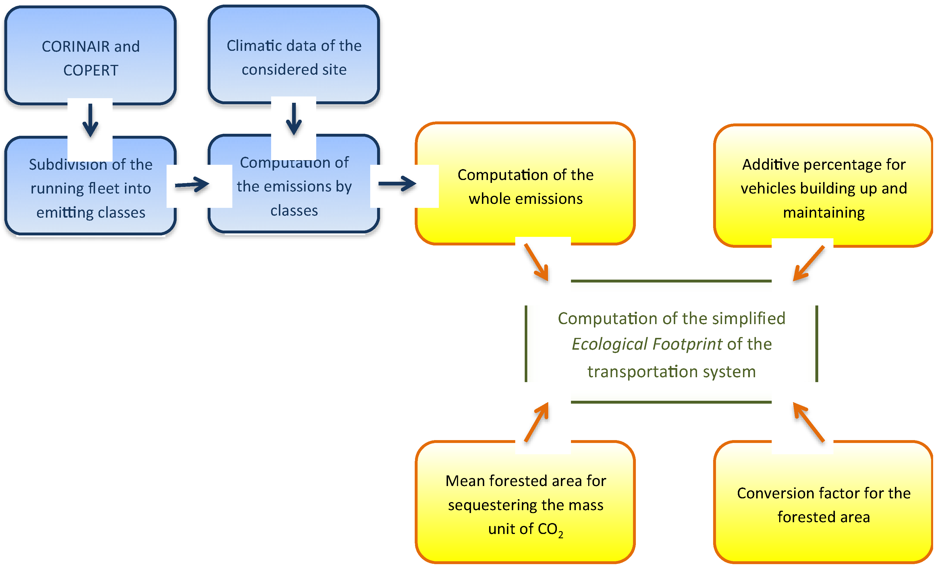
The whole method is based on a step-by-step procedure where parameters involved in the assessment of the ecological footprint are subsequently computed.

Figure 1 depicts the logical steps leading to the computation of the simplified ecological footprint of a given transportation system.

The emissions factors, for different average speeds and type of roads, are evaluated by means of the COPERT method [47,48], in order of evaluating the specific CO₂ emissions, A. That is:

$$A=\frac{{\text{CO}}_{\text{2}}\text{ emissions}}{\text{vehicle}\times \text{km}}\left[\frac{{\text{g}}_{{\text{CO}}_{\text{2}}}}{\text{veh km}}\right]$$

(1)

Figure 1. Logical flow chart for the computation of the ecological footprint of a given transportation system.

Figure 1. Logical flow chart for the computation of the ecological footprint of a given transportation system.

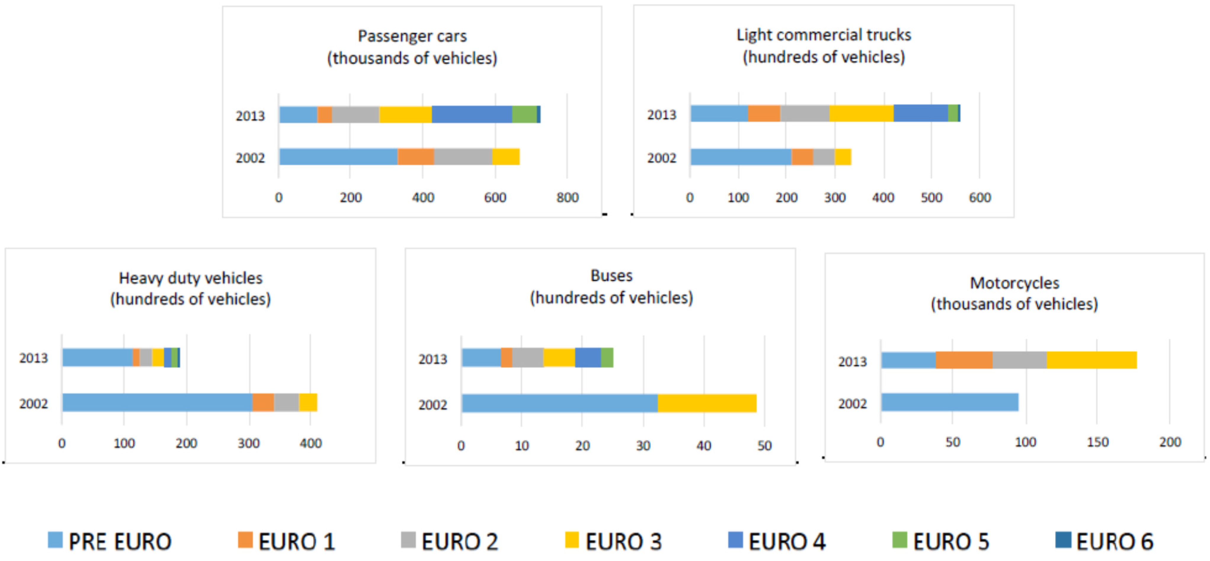
Data concerning the running fleet of the province was derived by official figures [49], by means of the subdivision of the whole fleet in suitable emitting classes, B. That is:

$$B=\text{number of vehicles by emitting classes\hspace{1em}}\left[\text{number vehicles}\right]$$

(2)

By simply multiplying the intensive parameter A by the extensive one; B, the CO₂ emissions of the province; C, are obtained for each emitting class:

$$C=A\cdot B={\text{CO}}_{\text{2}}\text{ emissions of Province\hspace{1em}}\left[\frac{{\text{g}}_{{\text{CO}}_{\text{2}}}}{\text{km}}\right]$$

(3)

Finally, the CO₂ emissions, D, of the whole province are simply computed as follows:

$$D={\displaystyle \sum _{\text{all classes}}C/1000=}{\displaystyle \sum _{\text{all classes}}{\text{CO}}_{\text{2}}\text{ emissions of the Province}=}\left[\frac{{\text{kg}}_{{\text{CO}}_{\text{2}}}}{\text{km}}\right]$$

(4)

Three more parameters are required in order of achieving the total footprint for the analysed system, that is E, F, and G. The first one, E, is the value of the mean forested area needed for sequestering one kg of CO₂. That is:

$$E=\text{Sequester factor for }{\text{CO}}_{\text{2}}\left[\frac{m^2}{{\text{kg}}_{{\text{CO}}_{\text{2}}}\cdot y}\right]$$

(5)

The value of this parameter is generally hypothesized to be 1.92 [32], taking into account that the conversion factor for the forested area, F, shows a mean value of 1.17 [50]. The productive area needed for the building up and the maintenance of a vehicle (15% of the total) and for the building up and maintenance of the road infrastructure (30% of the total) is considered as an additive parameter, G, assuming for it the cumulative value of 1.45 [32].

Finally, the ecological footprint of the province can be simply computed in terms of hectares of bio-productive soil attributed to a single vehicle travelling for one km, as follows:

$$I=\text{Province footprint}=D\cdot E\cdot F\cdot G/1000\left[\frac{\text{ha}}{\text{km}\cdot y\cdot \text{veh}}\right]$$

(6)

On turn, this value is also expressed in terms of m² of forested area needed for sequestering the CO₂ emissions released by the whole system.

It is important to observe that, in order of defining the parameter A, according to the COPERT method, an average value of speed of the involved transportation means is required. In the present analysis we have adopted the values [48] reported in Table 1: Ranges of main velocities refer to different classes of vehicles, depending on their volume capacity.

Table 1. Range of the average speed adopted for the transportation means in different types of roads.

Categories	Urban (km/h)	Rural (km/h)	Motorways (km/h)
Passenger cars	25	60–65	105–120
Light commercial trucks	25	65	95
Heavy duty vehicles	23	60	70–85
Buses	22	60	90
Motorcycles	30–34	60	100

Table 1. Range of the average speed adopted for the transportation means in different types of roads.

Categories	Urban (km/h)	Rural (km/h)	Motorways (km/h)
Passenger cars	25	60–65	105–120
Light commercial trucks	25	65	95
Heavy duty vehicles	23	60	70–85
Buses	22	60	90
Motorcycles	30–34	60	100

4. The Transportation Structure of the Palermo’ Province

The whole province of Palermo covers 4992 km² and has a population of 1,275,598 inhabitants. Referring to the town of Palermo, its transportation structure is quite complex, since it applies to a densely populated metropolitan area with 684,000 inhabitants.

Private cars are mainly used for urban mobility, both as drivers (32.4%) and as passengers (15.8%). A percentage of 11.7% of the population uses motorcycles and 12% uses public transportation means. Only 0.6% of population uses bikes, while the rest of the journeys are by foot [51].

Figure 2 refers to the running fleet of the Province of Palermo: in particular, the changes in the composition of the running fleet are shown for the years 2002 and 2013. These years have been selected due to the technical changes occurring in this period in the fleet, that led to significant modifications in the emitting properties of pollutants released by vehicles. In Figure 2, classes of vehicles and emitting categories are those contemplated within the COPERT methodology.

Figure 2 illustrates the specificity of the Palermo situation concerning the mobility of people. In fact, while the number of cars increases from 2002 to 2013 of about 7.36%, surprisingly the number of buses decreases as far as 49%. This is a consequence of the deep crisis that involved the public transportation company in the town of Palermo in those years, inducing people to apply to different means of transportation: not by chance, the number of motorcycles increased by about 85% in the same period.

Figure 2. Changes of the running fleet composition of the province of Palermo from 2002 to 2013.

Figure 2. Changes of the running fleet composition of the province of Palermo from 2002 to 2013.

5. Results

In order to get the values of the ecological footprint of the Palermo province transportation system, according to Equation (1), CO₂ emissions must be preliminarily computed. These data are obtained by utilizing the 2013 Emission Inventory Guidebook of European Environment Agency (EEA) [52]. The emitting properties of the analyzed metropolitan area are synthetically depicted in Table 2, in terms of number of vehicles and kg of CO₂ released by the vehicle fleets, for each km of the distance covered in the urban context.

An analysis of Table 2 suggests that two different trends can be found in the considered transportation system: on one hand, the number of vehicles for almost all the categories increased from 2002 to 2013, but heavy-duty trucks and buses; On the other hand the mean emissions of each vehicle representative of all categories show a relevant decreasing. The resulting effect of these opposite trends turns into the surprising values of the total CO₂ emissions, which from 2002 to 2013 decrease of only about 2.5%. This reduction is far to be relevant and confirms the specific environmental performances of the Palermo urban mobility. Therefore, the technological improvements of the fleet introduced with time (that would lead to a reduction of emissions) seem to be almost totally cancelled by the growth of the number of vehicles, leading to a quasi-constant emitting feature. In Table 2, for example, it is possible to note that, compared with a rise of about 7% of the number of cars emissions remain almost unchanged (showing only a rise of 0.9%). This is due to the fact that the average vehicle has improved its technological performances, moving from a mean release of 208 gCO₂/km (2002) to 192 gCO₂/km (2013).

These results, although significant for the description of the emission properties of the province of Palermo, show their limits when one desires to compare these performances with the environmental carrying capacity of the area. The Ecological Footprint, as previously established, aims to provide a comprehensive view on purpose.

Table 2. Running fleet and CO₂ emissions of the Palermo Province in the years 2002 and 2013.

Categories	Title	2002	2013	Δ%
Passenger cars	Vehicles number	669,732	719,023	7.36
	Total emissions (kgCO2/km)	139,462	138,180	−0.92
	Emissions of the average vehicle (gCO2/km)	208	192	−7.69
Light commercial trucks	Vehicles number	33,312	56,392	69.00
	Total emissions (kgCO2/km)	9927	15,515	56.00
	Emissions of the average vehicle (gCO2/km)	298	275	−7.72
Heavy duty vehicles	Vehicles number	40,925	18,678	−54.00
	Total emissions (kgCO2/km)	27,237	12,163	−55.00
	Emissions of the average vehicle (gCO2/km)	666	651	−2.25
Buses	Vehicles number	4873	2506	−49.00
	Total emissions (kgCO2/km)	3222	1483	−54.00
	Emissions of the average vehicle (gCO2/km)	661	591	−10.60
Motorcycles	Vehicles number	95,571	176,426	85.00
	Total emissions (kgCO2/km)	10,484	18,135	73.00
	Emissions of the average vehicle (gCO2/km)	110	103	−6.36
Running fleet	Total emissions (kgCO2/km)	190,333	185,476	−2.55

Table 2. Running fleet and CO₂ emissions of the Palermo Province in the years 2002 and 2013.

Categories	Title	2002	2013	Δ%
Passenger cars	Vehicles number	669,732	719,023	7.36
	Total emissions (kgCO2/km)	139,462	138,180	−0.92
	Emissions of the average vehicle (gCO2/km)	208	192	−7.69
Light commercial trucks	Vehicles number	33,312	56,392	69.00
	Total emissions (kgCO2/km)	9927	15,515	56.00
	Emissions of the average vehicle (gCO2/km)	298	275	−7.72
Heavy duty vehicles	Vehicles number	40,925	18,678	−54.00
	Total emissions (kgCO2/km)	27,237	12,163	−55.00
	Emissions of the average vehicle (gCO2/km)	666	651	−2.25
Buses	Vehicles number	4873	2506	−49.00
	Total emissions (kgCO2/km)	3222	1483	−54.00
	Emissions of the average vehicle (gCO2/km)	661	591	−10.60
Motorcycles	Vehicles number	95,571	176,426	85.00
	Total emissions (kgCO2/km)	10,484	18,135	73.00
	Emissions of the average vehicle (gCO2/km)	110	103	−6.36
Running fleet	Total emissions (kgCO2/km)	190,333	185,476	−2.55

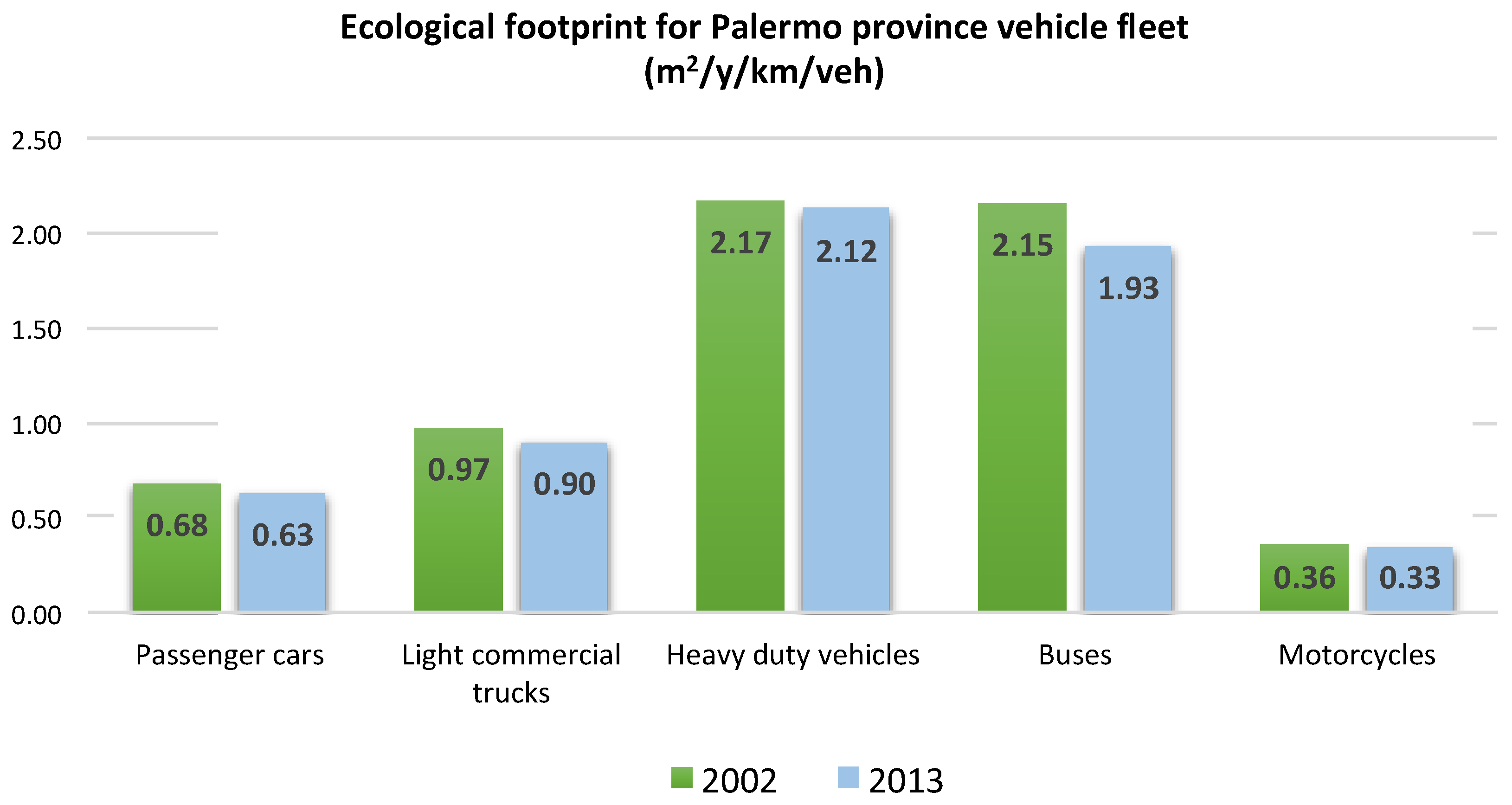
In fact, the simplified version of the ecological footprint methodology is here applied to the transportation system of the Palermo province with the aim of singling out the equivalent surface of bio-productive land needed for sustaining the urban mobility system. The results of these calculations, for years 2002 and 2013, are summarised in Figure 3 in terms of surface of forested area needed for sequestering the CO₂ emissions of this transportation system. Figure 3 refers to the footprint of each representative vehicle of all emitting categories.

Results directly reveal the features of the emission system, as reported in terms of CO₂ releasing in Table 2. In fact, despite the technological improvements certainly introducing a reduction in the emissions of each single vehicle, the increasing number of the total vehicles results in an almost constant environmental performance.

In order to get a unique indicator of the sustainability performance of the area, compared with its carrying capacity, one can add the values of the ecological footprint of each category of emitting vehicles. The total values of the ecological footprint of the whole transportation system if, for example, each vehicle is supposed to travel one km/year, are 62 and 60.41 ha/(km·year) for the years 2002 and 2013, respectively.

Referring to car mobility, values of surface of equivalent forested land needed to absorb the CO₂ emissions of this subsystem, per each single travelled km by the average car of the fleet, are 0.68 and 0.63 m²/(km·year) respectively for the years 2002 and 2013. These figures are comparable with those earlier found for the UK [32], that ranged from 0.73 (low scenario) to 0.90 (medium scenario). Anyway, in order to better compare the actual situation of the passenger car subsystem, it is interesting to report its ecological footprint by better referring to the occupational rate of these vehicles. This further examination shows that, by considering a mean occupation rate of 1.2 passengers per car, the footprint of cars in the province of Palermo accounts for 0.57 and 0.52 m²/(km·year·pass), respectively for the years 2002 and 2013.

Figure 3. Ecological footprint for the running fleet of the Palermo Province for years 2002 and 2013.

Figure 3. Ecological footprint for the running fleet of the Palermo Province for years 2002 and 2013.

These data are surely interesting, since they give a direct overview of the trend with time of the emissions properties of the given mobility fleet. This way of describing the environmental features of the transportation system, allows comparing its trend with the actual carrying capacity of the considered territory. This is easily provided, in fact, by the ecological footprint approach that enables the evaluation of the pressure exerted by the mobility system on the ecological reservoirs of the territory to which the urban context belongs.

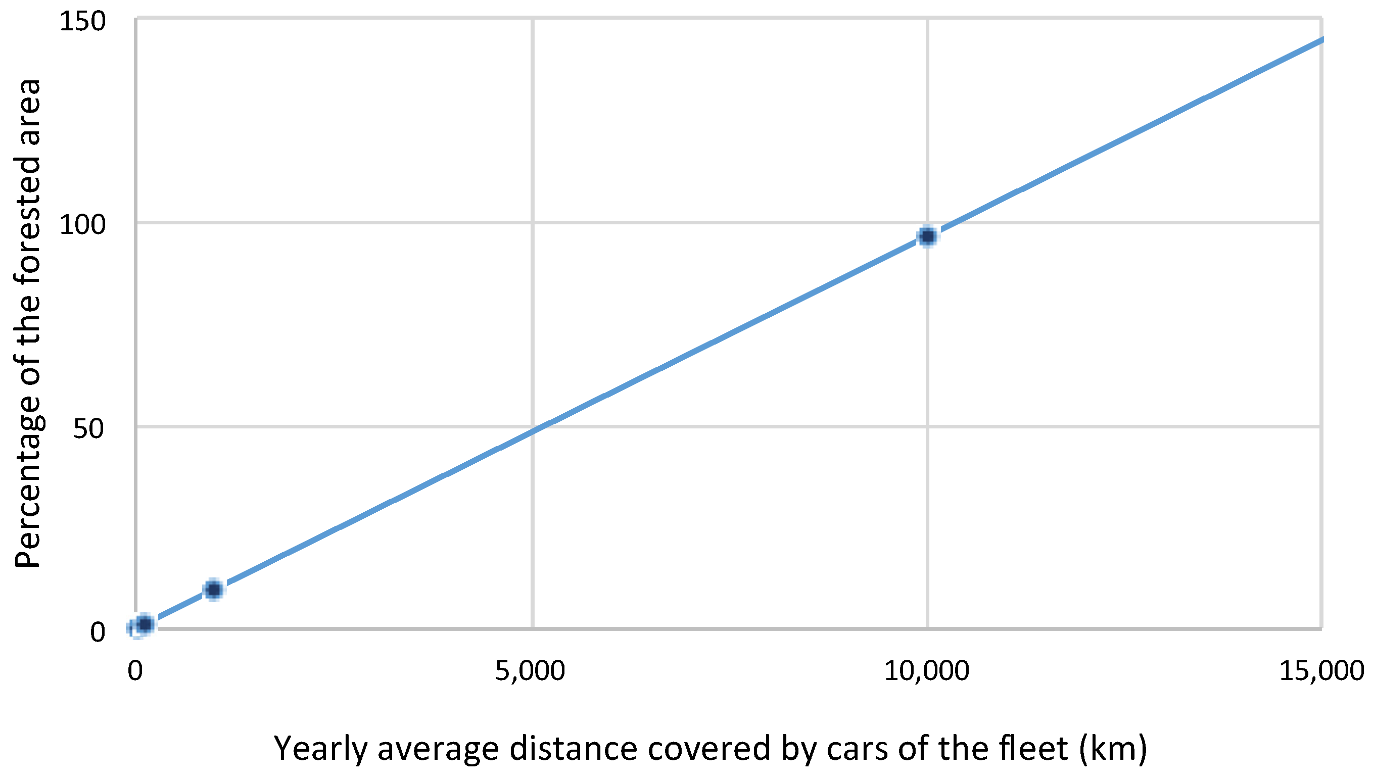
By referring, for example, to the ecological footprint of the average car of the fleet of the Palermo province, it is now easy to evaluate its impact on the environment, in terms of surface of forested area needed to absorb the yearly CO₂ emissions of the fleet. Figure 4 indicates, for different yearly trip lengths of the car, the percentage of forested surface needed for sequestering the corresponding emissions, taking into account that the total forested surface of the province is about 67,000 hectares. As it is possible to note, if all cars of the province would travel 10,000 km/year, they would sequester almost the total forested surface of the province. Luckily, the mean trip yearly covered by the average car of the Palermo fleet is about 7000 km, with a decreasing trend of 17% per year in the last two years [53]. Nevertheless, this value clearly signals the need for deep policy interventions in the mobility system of the Palermo province.

These considerations suggest that not only are the technological changes of the vehicle fleet the key in reducing the energy footprint of traffic, but also there is needed the integration of other actions.

Another relevant advantage of the use of the ecological footprint method is the possibility to comparatively evaluate the environmental performances of different transportation systems, in this way establishing a sort of general method for hierarchizing various urban contexts. In this aim, we have here applied the methodology to three further Italian provinces (apart Palermo, 1,275,598 inhabitants), that is Milano (3,176,180 inhabitants), Mantova (415,147 inhabitants), and Bolzano (515,714 inhabitants). These have been selected as representative of big (Milano), medium (Bolzano), and small (Mantova) Italian urban settlements. From an environmental point of view, these contexts performed differently since, in the last country report concerning the environmental quality of Italian towns [54] for the year 2014, Milano and Palermo were respectively the 3rd and the 14th biggest urban areas, Bolzano was the 8th of the medium areas, and Mantova was 10th of small ones.

Figure 4. Percentage of the forested area of the Palermo province needed for sequestering the CO₂ emissions of the whole car fleet, for various yearly covered distances.

Figure 4. Percentage of the forested area of the Palermo province needed for sequestering the CO₂ emissions of the whole car fleet, for various yearly covered distances.

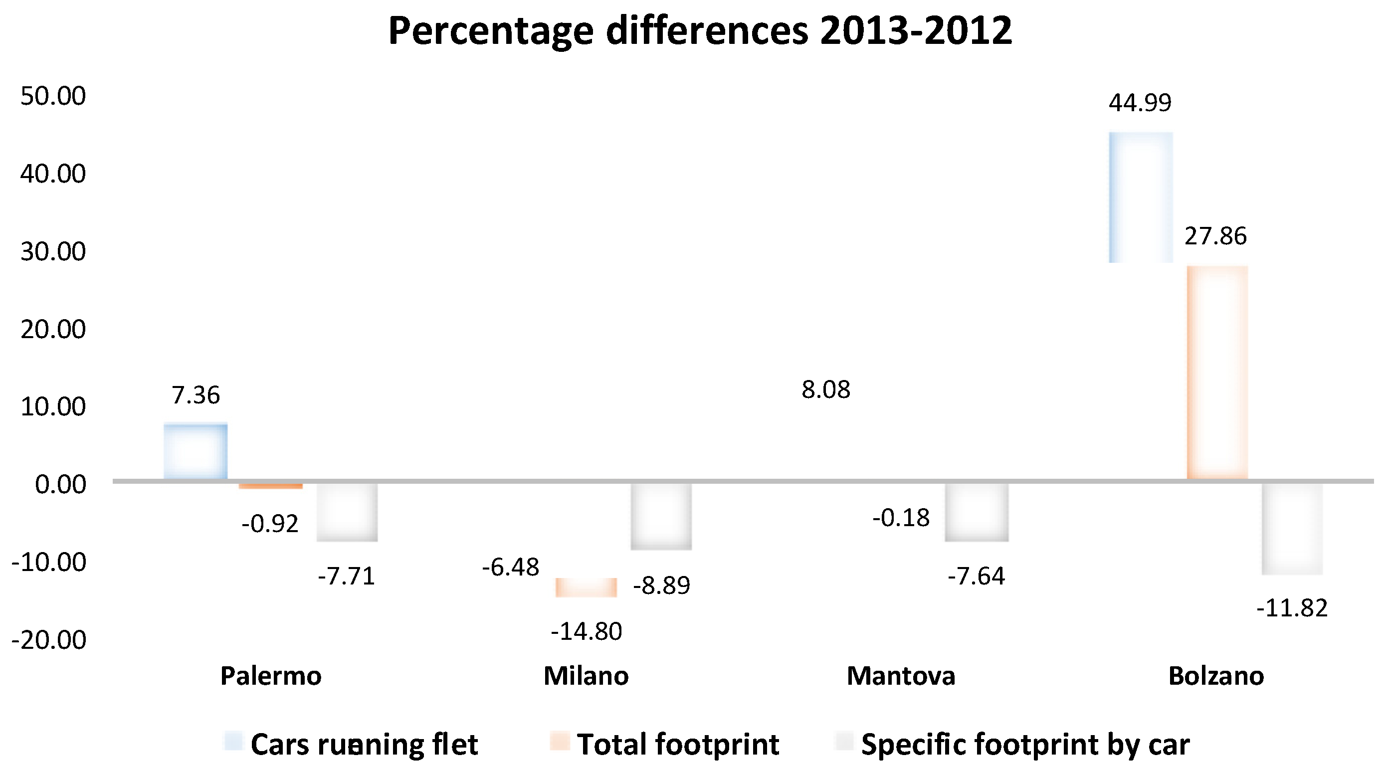
Figure 5 reports the percentage changes of the total [ha/(year·km)] and specific [m²/(year·km·veh.)] footprints of the four provinces, as a function of the changes in their car fleets. The total footprint can be utilized for comparatively analysing the performances of the transportation system of the four provinces, while the specific footprint is a synthetic indicator of the technological improvements of their car fleets.

First of all, it is important to note the huge increase of the car fleet of Bolzano: this is justified by the significant growth of the cumulated GDP of this province in the years from 2002 to 2010 (+38.4%) compared with those of Lombardia (+34.58)—to which Milano and Mantova belong—and Sicily (+27.23%)—to which Palermo belongs. The corresponding cumulated change in the GDP of Italy was +30.77%. Moreover, in the period 2010–2012, just in the middle of the economic crisis, the province of Trentino (including Bolzano) has shown an increment in its GDP of 3.3%, compared with a mere +0.9% in Lombardia and a 0.24% decrease in Sicily.

Concerning the technological improvements of the car fleets, Figure 5 clearly tells that Bolzano has achieved the best result between the years 2002 and 2013: in fact, despite a rising of about 45% of its running fleet, this province presented a decrease of about 12% of the footprint of the average car of the fleet. Palermo and Mantova show an almost similar result, with a decrease of about 7% of the footprint of the single average vehicle in spite of a rising of about 8% of their running fleets. Milano presented the worst performance, since it achieved a decrease of only about 9% of the specific footprint, notwithstanding the car fleet correspondingly decreased its number of vehicles of about 6%.

When the performances of the average cars are combined with the total numerical consistence of the running park, one obtains an immediate view of the whole outcome of the provinces. Figure 5 illustrates these results, showing that, for the period between years 2002 and 2013, Milano reached the best position, with a decrease of almost 15%. Palermo and Mantova have shown a small decrease (respectively, −0.92% and −0.18%), while Bolzano, due to the enormous growth of its fleet, registered an increase of about 27% of the ecological footprint.

Figure 5. Changes between years 2002 and 2013 of the total and specific footprints of four Italian provinces, compared with the corresponding changes of car fleets.

Figure 5. Changes between years 2002 and 2013 of the total and specific footprints of four Italian provinces, compared with the corresponding changes of car fleets.

Ecological footprint, as shown for Palermo, also presents an interesting feature of allowing the association of the performances of a given transportation system with the carrying capacity of the territory where the system is supposed to act. In order to comparing the four analyzed provinces, we have here hypothesized that each single car of the fleet would run, as average, 5000 km/year. In this way, the ecological footprint of each transportation system can be simply compared with the surface of the province to which it belongs. Table 3 illustrates these comparisons: Mantova and Bolzano affect only a small percentage the environmental reservoir of their provinces, while Palermo and Milano have worse performances, indicating a use of the territory greater of its surface.

Table 3. Running fleet and CO₂ emissions of the Palermo (Province) in the years 2002 and 2013.

Province	Surface (ha)	Total Footprint (ha/5000 km)	Ratio Footprint/Surface
Palermo	157,890	225,045	1.425
Milano	233,800	553,236	2.366
Mantova	739,900	77,046	0.104
Bolzano	499,200	106,335	0.213

Table 3. Running fleet and CO₂ emissions of the Palermo (Province) in the years 2002 and 2013.

Province	Surface (ha)	Total Footprint (ha/5000 km)	Ratio Footprint/Surface
Palermo	157,890	225,045	1.425
Milano	233,800	553,236	2.366
Mantova	739,900	77,046	0.104
Bolzano	499,200	106,335	0.213

Clearly, should have these comparisons been referred to the forested areas, instead of the whole province surfaces, we would have obtained worse results: anyway, this simple application demonstrates the feasibility of the ecological footprint method not only for analyzing the environmental performances of a given transportation system, but also for comparing and ranking different systems operating in various territorial contexts.

6. Discussion

The proposed integrated method, for the evaluation of the pressure exerted by urban transportation systems on a given territory, suggests some further considerations, particularly concerning its applicability to other different contexts and regarding lessons learned from the study.

The method has been applied to a set of Italian provinces, selected on the basis of their population and the performances of their respective transportation systems. Results have spotlighted the trends of these provinces, from years 2002 and 2013, showing good ability of the method in capturing the effects produced by the changes in the numerical composition of the vehicular fleets and by the technological improvements that better the emissive properties of the fleets. Anyway, the applicability of the method to other situations and contexts needs to be verified with respect: (1) to its feasibility for transportation systems belonging to other countries and (2) to the possibility of applying the methodology to single towns instead of entire provinces.

The applicability of the proposed methodology to other different contexts is simply guaranteed by its calculation scheme. In fact, it relies on data referring to specific pollutant emissions (see Equation (1)) of vehicles (g_pollutant/km): these parameters are provided by the European Environment Agency (EEA) [52] for the European context by means of the 2013 release of EMEP/EEA Emission Inventory Guidebook [55]. Obviously, the availability of such a detailed and up-to-date study puts the research of European countries in a clear advantaged position. Anyway, all around the world, almost all countries have assessed specific studies for defining the pollutant emissions of their transportation systems. On purpose, we can cite the pioneer work of Faiz et al. [56] that pointed out their attention on the emissions from motor vehicles of several non-European countries. Concerning the European non-EU countries (Albania, Belarus, Bosnia-Herzegovina, Croatia, Macedonia, Moldova, Norway, Russia, Serbia-Montenegro, Switzerland, Turkey, and Ukraine), a study of the International Institute for Applied Systems Analysis (IIASA) [57] expressly indicates, within the emission control measures to be assumed, the EURO 4 standards for cars and light-duty trucks, in this way acknowledging the validity of the COPERT scheme also for these countries. More in general, the Intergovernmental Panel on Climate Change (IPCC) [58] reports a worldwide approach for mitigating the emissions from transport and its infrastructures. Finally, Eggleston and Walsh [59] suggest a comparison between IPPC vehicle types and COPERT classes: it is interesting to note that the mean CO₂ emission factors (gCO₂/kg of fuel) for road transport are 3172 and 3180, respectively for US and Europe, in this way indirectly confirming the validity of the European method.

In conclusion, it is possible to confirm that several countries in the world are currently arranging their vehicle data in a way that makes the application of the simplified method here proposed possible.

Referring to the possibility of applying the integrated method to single towns, instead of whole provinces, it must be noted that data concerning the composition of the vehicular fleets are usually available as part of the statistical database of countries. Such data, in fact, are compiled and up-to-date also for fiscal purposes. This means that the emissive classes of vehicles can be easily assessed also for towns, making the application of the method generally possible.

However, what are the lessons learnt by the application of this method to different urban contexts? We believe that they rely on two kinds of ambits.

On one hand, the method has shown its feasibility in allowing an easy and reliable evaluation of the environmental pressure exerted by transportation systems characterized by different vehicular fleet composition. Moreover these evaluations can be comparatively performed, so enabling a useful hierarchizing of different contexts. This feature can be utilized for indicating to a given territorial context (province, town, etc.) the distance from the actual benchmark, in this way pushing for the introduction of proper changes in the structure of the transportation system (for example, inducing a useful shift toward a better public/private share of the urban mobility). In addition, central administrations can benefit from these rankings, in order of better assign budgets to municipalities in terms of environmental performances of their mobility systems.

On the other hand, the method, thanks to its easy to use structure, can be conveniently utilized as a design tool for territories where significant transportation systems are present. In fact, administrators need to have at their disposal simple but reliable methods able to embody in the planning process the effect produced by different scenarios of transportation systems. The simplified ecological footprint scheme here proposed seems to accomplish this requirement, particularly due to its characteristic of matching the burden of a given transportation configuration with the environmental reservoirs of the interested territory.

7. Conclusions

By means of a simplified application of the ecological footprint method, the environmental performances of the mobility system of the province of Palermo have been evaluated.

The method, compared with the classical analysis based on the assessment of the pollutants released by transportation, allows the direct matching of the performances of the system with the carrying capacity of the environment where it is supposed to act. In fact, the European policies concerning a “roadmap towards a competitive and resource-efficient transport system” [21] put limits on the greenhouse gas (GHG) emissions from the transportation referring to the whole planet sustainability. Actually, the emissions should be also compared with the capability of supporting these pressures by the surrounding environment. The ecological footprint method provides an answer to this need, by comparing the emissions from transports with the carrying capacity of the specific site.

This feature of the method candidates it as a tool for comparing different policy actions in the transportation system. In fact, referring to the province of Palermo, the ecological footprint analysis, apart from indicating the important role played by individual mobility (cars), could be usefully employed for assessing the change in the environmental burden subsequent to different transport scenarios. In the present case study, the ecological footprint has decreased only of a percentage of 2.55% in 11 years: the reasons of this result have been analyzed through the paper. Anyway, this result is far from the goals of EU which has called for reducing emissions by 80%–95% below 1990 levels by 2050 [21]. These goals are clearly threatened, given the substantial increase of transportation emissions over the past two decades, that would still put them at 8% above the 1990 level.

Concerning the policies to be adopted by an administration in order of improving the environmental performances of a transportation system, a relevant role could be plaid for example, by the modification of the urban modal split, by discouraging private cars in favor of public or more sustainable mobility solutions.

Referring to further studies to be undertaken with the aim of improving the reliability of the method, the importance of including an accurate analysis of the footprint of the road surface in the computation of the ecological footprint of the system must be cited. Moreover, the percentage of footprint attributed to the building up and maintenance of vehicles should be better defined, in order to more precisely refer to the actual composition of a given running fleet.

Anyway, the ecological footprint method has shown to be an effective tool for comparing different configurations of an urban transportation system.