Gain Scheduling Control of an Islanded Microgrid Voltage

Abstract

The aim of this research study has been to design a gain scheduling (GS) digital controller in order to control the voltage of an islanded microgrid in the presence of fast varying loads (FVLs), and to compare it to a robust controller. The inverter which feeds the microgrid is connected to it through an inductance-capacitor-inductance (LCL) filter. The oscillatory and nonlinear behaviour of the plant is analyzed in the whole operating zone. Afterwards, the design of the controllers which contain two loops in cascade are described. The first loop concerns the current control, while the second is linked to the voltage regulation. Two controllers, one defined as Robust and another one as GS controller, are designed for the two loops, emphasizing in their robustness and their ability to damp the oscillatory plant behaviour. To finish, some simulations are carried out to study and compare the two kinds of controllers in different operating points. The results show that both controllers damp the oscillatory behaviour of the plant in closed loop (CL), and that the GS controller ensures a better rejection of current disturbances from FVLs.

1. Introduction

There exist more and more proposals to organize some parts of the power system as microgrids (MGs), in particular in rural or island regions. A microgrid can be defined as a weak electric grid formed by different renewable sources, auxiliary sources, energy storage systems, power converters, loads and control systems. Generally, microgrids are not opposite but complementary to the interconnected power system. They can be as efficient and self-sufficient as possible, and they can island rapidly during emergencies [1]. However, when operating in islanded mode, they become weak grids and are thus less stable and more vulnerable to variable sources and loads.

Many different issues concerning control in islanded MGs can be found in the scientific literature. One of them concerns frequency regulation. For instance in [2], the increase of the frequency stability of islanded microgrids during both primary and secondary frequency control is carried out through a cooperative frequency control method. In [3], single master and multi master operations are tested. Simulation results show that both control strategies are effective and ensure efficient and stable MG operation.

Another typical issue is related to power quality. In [4], two improved control strategies associated to a three-phase, four-leg distributed generation grid-interfacing converter, are proposed. They have the capacity to compensate current harmonic, provide proper power sharing in the MG, reduce the degree of voltage unbalance and eliminate the impact of voltage sags, voltage swells, and distortions in the utility grid on the micro-grid when transitioning from grid-connected mode to islanded mode. The voltage unbalance issue is also considered in [5], where the distributed generation units are operated by the voltage-based droop control and an additional control loop for unbalance mitigation and sharing.

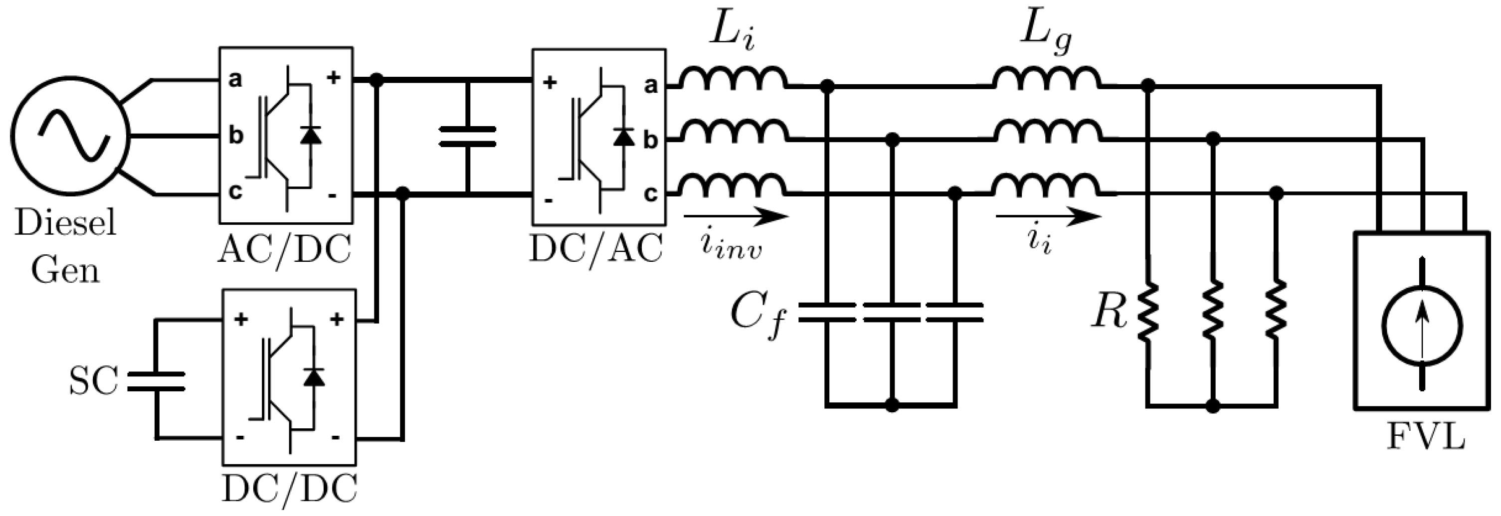
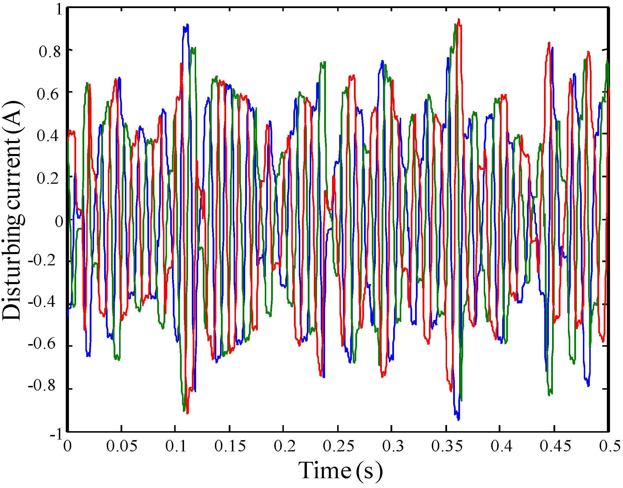
The aim of this research study is to design robust controllers to control, via an inverter associated to an inductance-capacitor-inductance (LCL) filter, the voltage of a mostly resistive isolated microgrid disturbed by Fast Varying Loads (FVL) (see Figure 1).

Most of the elements of a microgrid are interconnected through power converters, which allow controlling the power flow of each element. In this context, inverters play a vital role in order to keep the stability of the microgrid. An inverter can use different types of passive filters to eliminate the harmonics generated by the commutation. Mainly three types of filters are used, inductance (L), inductance-capacitor (LC) or LCL [6].

The L filter is the simplest one from the point of view of the design and control. However, if the power is higher than several kilowatts, the value of the inductance should be high enough to eliminate the harmonics and therefore the price would be high too [7]. Furthermore, a high inductance would deteriorate the dynamic response of the system and due to the high voltage loss it would be necessary to increase the direct current (DC) bus voltage [8].

A capacitor may be connected in parallel with the inductance to form an LC filter, which allows reducing the size of the inductance. However, the value of the capacitor should be high enough to reduce the size of the inductance, which is not recommended due to the high inrush currents and high reactive currents that it would generate as well as the dependence of the filter on the grid impedance [9].

The LCL filter is the most used one as it has a good harmonic attenuation using low size, and therefore low price, passive elements in comparison with the other types of filters. Besides, the dependence on the grid impedance is lower than in the case of the LC filter [9]. However, this kind of filter usually makes its electrical variables being oscillatory. This fact has to be considered when designing the inverter controller.

The design of the controller of an inverter that uses an LCL filter is carried out in several research works assuming that the effect of the capacitor is low enough to neglect it, knowing that due to the bandwidth of the controller, it only affects to the current harmonics of low order [10,11]. In these references, once a proportional-integral (PI) type controller is designed, its stability is analyzed using the complete dynamic model of the LCL filter. Passive [7] or active [12] damping methods are used to minimize the effect of the inherent resonance of the filter.

The control of the inverter is generally based on two regulation loops, an inner one of current (the current of the converter or alternatively the current of load side inductance is controlled by this loop) and an external one of voltage or power (the one of converter or load side). If the current of the converter side inductance is controlled, the obtained system is more stable than the system obtained controlling the load side inductance current. The feedback of the converter side inductance current inserts an attenuation of the resonance of the filter [13]. However, if the objective of the outer loop is to control the voltage or the power of the load, this strategy implies that the outer loop control model has also a resonance.

In this work the inner loop has been designed to control the current of the load side inductance, and the outer loop to control the voltage of the microgrid. As analyzed in Section 2, the isolated/islanded nature of the microgrid induces a nonlinear behavior of the plant. To face this non-linearity, on top of a robust controller, an adaptive/gain scheduling (GS) controller is designed. The main objectives of these controllers are to damp the oscillating dynamic of the plant, to reject disturbances and to obtain robustness in stability, dynamic characteristics and in stability margins on the entire operation zone of the plant.

The remainder of this paper is organized as follows: Section 2 describes the considered microgrid and the current disturbances occurring there, the dynamic model of the plant and an analysis of the nonlinearity of the model. Section 3 explains the design of the two controllers of the inverter. Section 4 shows and analyses some simulation results carried out to test the quality of the designed controllers. Finally, Section 5 gives the conclusions related to this work.

2. Plant Analysis

This section is formed by three sub-sections. In the first one, the considered microgrid and the occurring current disturbances are described. Then, in the second sub-section, the dynamic model of the plant is explained. In the third one the nonlinearity of this plant is analyzed.

2.1. Description of the Studied Microgrid

Figure 1 shows the structure of the studied microgrid, including the inverter with an LCL filter. The values of its components are shown in Table 1, with other parameters. E_n is the RMS voltage between two phases, V_dc is the DC bus voltage, P_n is the inverter nominal power, R_nom is the resistive load value corresponding to the nominal power, f is grid frequency, f_com is the inverter commutation frequency and L_i, C_f and L_g are respectively the LCL filter related inverter-side inductance, the capacitor and the grid-side inductance parameters. These values are those of the experimental microgrids of the Genie Electrique et Automatique aux Service des Energies Renouvelables (EneR-GEA) research group [14]. They correspond to a low-power microgrid but the analysis and the controller designing process carried out in this paper could be applied to real-size microgrids.

As shown in Figure 1, the operation of the microgrid has been analyzed in grid-disconnected case. In this configuration, the microgrid needs a reliable power source that will assure the correct supply of energy/power to keep the operation of the microgrid stable. In the analyzed case a Diesel Generator has been used to satisfy this requirement, in parallel with a SuperCapacitor (SC) bank. The Diesel Generator supplies power to the loads and keeps constant the amplitude and frequency of the weak grid. A supercapacitor bank, controlled by a DC–DC converter, is used to face the fast power variations that may come from the elements connected to the microgrid. As depicted in Figure 1, the considered microgrid is mostly resistive. However, other types of loads that can interfere in the operation of the microgrid have been considered as well, such as Fast Varying Loads (FVL) [15]. The active and/or reactive power consumption of the FVL varies very fast, as in the case of crushers, rolling mills, electrical excavators or spot welders. As explained in [15], these kinds of loads can be classified as repetitive, random or burst FVL. The FVL have been represented using current sources.

Figure 1. Structure of the studied microgrid.

Figure 1. Structure of the studied microgrid.

Table 1. Parameters used in simulations.

Parameter	Parameter name	Value
RMS line voltage	En	400 V
DC bus voltage	Vdc	900 V
Inverter nominal power	Pn	2000 W
Nominal resistive load	Rnom	79.35 Ω
Grid frequency	f	50 Hz
Inverter commutation frequency	fcom	5 kHz
Filter inverter-side inductance	Li	3 mH
Filter capacitor	Cf	2 µF
Filter grid-side inductance	Lg	3 mH

Table 1. Parameters used in simulations.

Parameter	Parameter name	Value
RMS line voltage	En	400 V
DC bus voltage	Vdc	900 V
Inverter nominal power	Pn	2000 W
Nominal resistive load	Rnom	79.35 Ω
Grid frequency	f	50 Hz
Inverter commutation frequency	fcom	5 kHz
Filter inverter-side inductance	Li	3 mH
Filter capacitor	Cf	2 µF
Filter grid-side inductance	Lg	3 mH

In this work the focus has been placed on the operation of the DC/AC inverter shown in Figure 1. It has been assumed that the Diesel Generator is able to supply the necessary average power to the loads and the supercapacitor (SC) bank and its DC/DC converter face fast power variations to keep the DC voltage constant.

2.2. Modeling of the Plant

The dynamic model of the LCL filter is formed by three differential Equations (1)–(3), where the variables are represented per phase j = a, b or c. i_inv is the current of the inductance L_i, i is the current of the inductance L_g, V_c is the voltage of the capacitors C_f and m is the duty cycle:

(1)

(2)

(3)

These differential equations, referenced in the abc reference system, can be transformed to the rotating dq reference system, obtaining the Expressions (4)–(6). In these new expressions the variables i_inv, i, V_c and m are spatial vectors and they are shown in bold; ω_s is the angular frequency of the grid:

(4)

(5)

(6)

The differential Equations (4)–(6) are used to obtain the transfer functions that are used to design the control systems after. The needed transfer functions are the ones that relate the d and q components of the current of the load with the d and q components of the duty cycle signals. These transfer functions are shown in Equations (7) and (8). They have the same Expression:

(7)

(8)

2.3. Analysis of the Nonlinearity of the Plant

As it can be seen in Equations (7) and (8) the plant is nonlinear. Indeed, the transfer function between m_d or m_q and i_d or i_q depends on the value of the resistive load of the isolated microgrid. This Section analyses the dynamic behavior of the plant at different operation points which are related to different resistance values between R_nom and 10 R_nom.

Figure 2 shows the response of the system to a unity step of m_d at different operation points. It can be seen that the gain of the system is smaller when the resistance increases. Furthermore, it can be also seen that the damping of the system is higher when the resistance is smaller. Concerning the frequency of the oscillations, they are similar in the entire operation zone.

Figure 3 shows the Bode diagram of the plant for different resistance values. The diagram confirms the analysis carried out in Figure 2: the plant has a smaller gain and it is less damped when R increases, i.e., when the consumed power is smaller.

Figure 2. Time response of the plant when a unity step of m_d is applied at different operation points (R_nom, 1.5 R_nom, 2 R_nom, 3 R_nom, 4 R_nom, 5 R_nom, 6 R_nom, 7 R_nom, 8 R_nom, 9 R_nom, 10 R_nom).

Figure 2. Time response of the plant when a unity step of m_d is applied at different operation points (R_nom, 1.5 R_nom, 2 R_nom, 3 R_nom, 4 R_nom, 5 R_nom, 6 R_nom, 7 R_nom, 8 R_nom, 9 R_nom, 10 R_nom).

Figure 3. Bode diagram of the plant at several operation points (R_nom, 1.5 R_nom, 2 R_nom, 3 R_nom, 4 R_nom, 5 R_nom, 6 R_nom, 7 R_nom, 8 R_nom, 9 R_nom, 10 R_nom).

Figure 3. Bode diagram of the plant at several operation points (R_nom, 1.5 R_nom, 2 R_nom, 3 R_nom, 4 R_nom, 5 R_nom, 6 R_nom, 7 R_nom, 8 R_nom, 9 R_nom, 10 R_nom).

It can be also seen that the resonance frequency is similar for all R values, inside the defined range (the maximum resonance frequency is 1.4 × 10⁴ rad/s).

3. Controller Design

This section presents the way the two controllers compared in this paper are designed. The first is defined as the “Robust controller”. The second one is an improved controller containing a GS strategy.

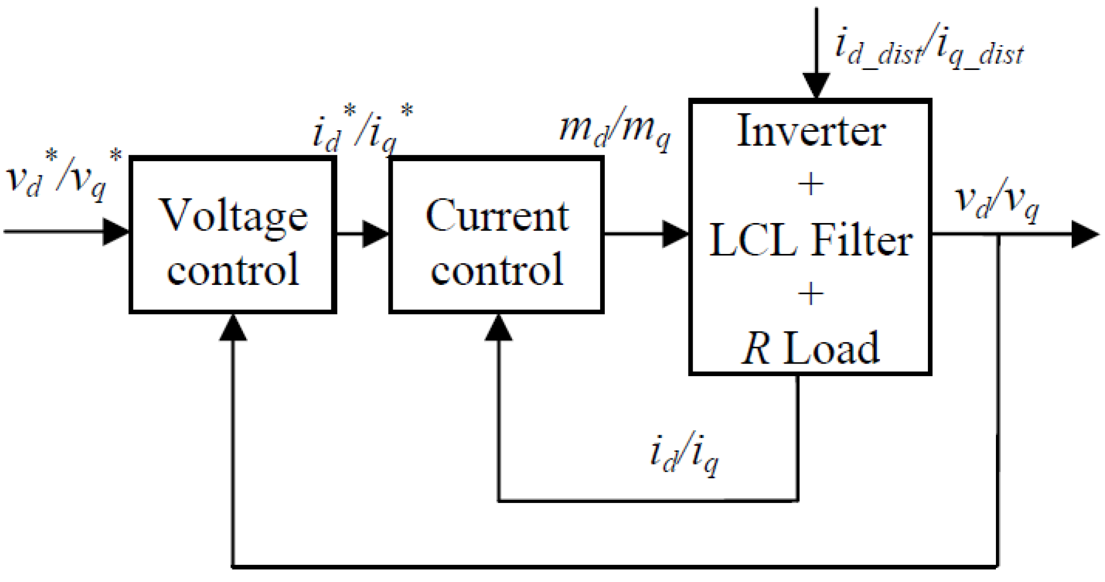
Both controllers are based on two loops in cascade, as depicted in Figure 4. The inner loop controls the LCL filter output current in d and q axes through the duty cycle signals m_d and m_q. i_{d_dist} and i_{q_dist} represent the plant output disturbance current, specially generated by the FVL, in d and q axes. The inner control law design is described in Section 3.1.

The outer loop regulates the inverter filter output voltage in d and q axes, generating i_d^* and i_q^* current references for the inner loop. The related control law design is described in Section 3.2.

Figure 4. Controllers structure in the dq reference axes.

Figure 4. Controllers structure in the dq reference axes.

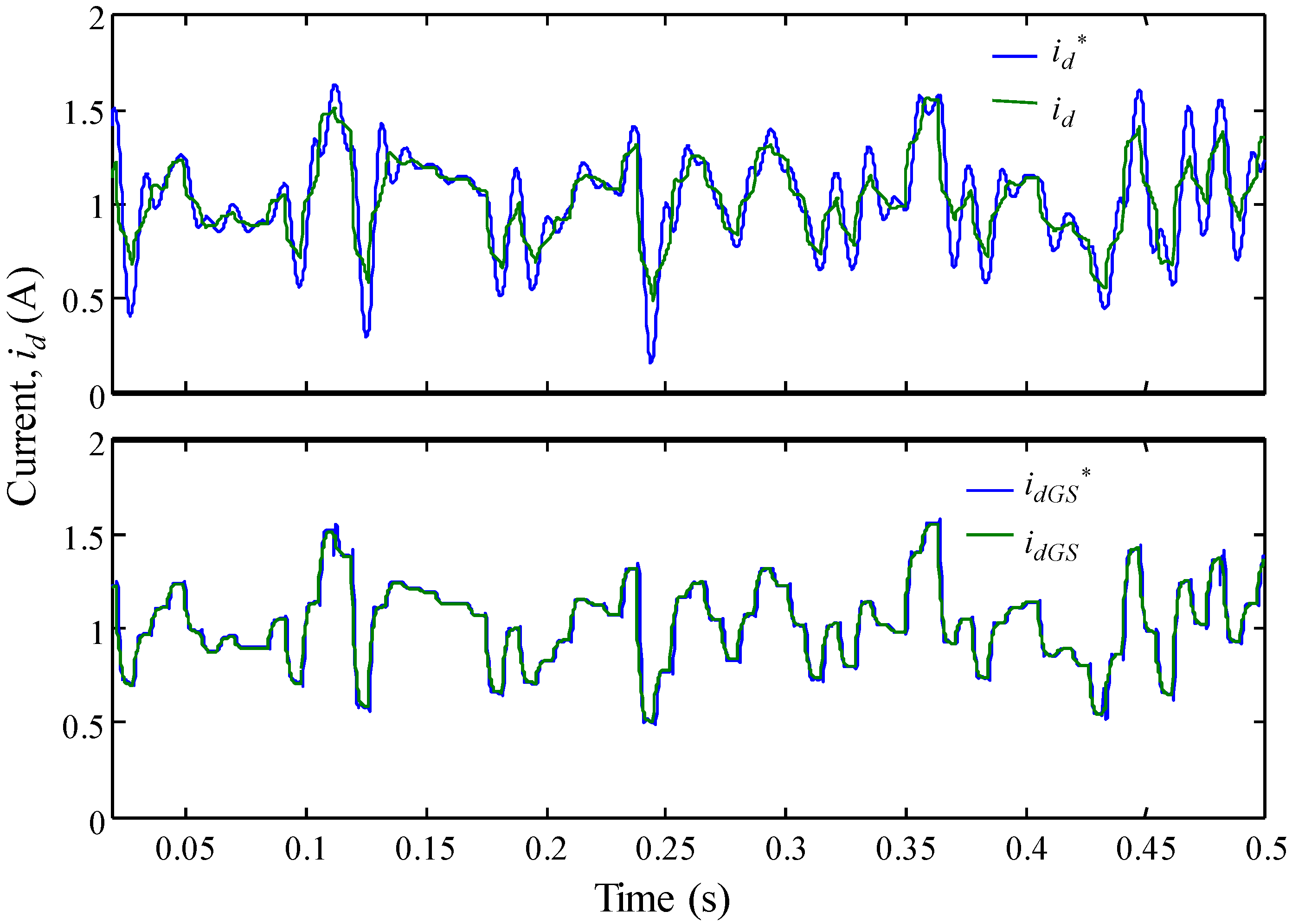
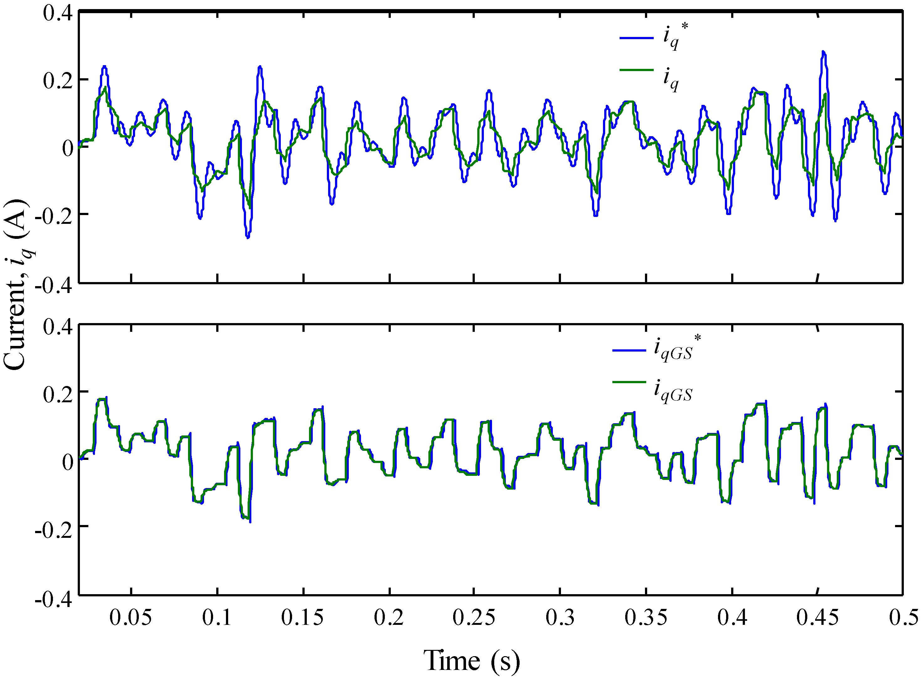
3.1. Current Loop

3.1.1. Control Objectives

The controller of the current loop aims to control i_d and i_q through m_d and m_q control signals. As seen in Section 2.3, the plant has an oscillating behavior. The desired dynamical performances are defined in order to damp this behavior, and to obtain a response as fast as possible to reject the output current disturbances. Regarding static specifications, no static error is desired in response to a step of reference and disturbance. As seen in the analysis carried out in Section 2.3, the plant behavior is nonlinear in the operating zone. Thus, another objective of the controller is to be robust enough in stability in the whole zone, with a modulus margin upper than −6 dB and a delay margin higher than one sample time. On top of these specifications, the GS controller aims also to keep a similar settling time in the whole operating zone.

3.1.2. Control Model

A continuous-time plant model has been obtained analytically in Section 2.2. The control model is calculated digitizing the continuous transfer functions. For that, the sampling time is selected in order to respect two conditions:

• It should be small enough to eliminate the oscillations of the plant. More precisely, the sampling frequency has to be at least twice higher than the maximum resonance frequency of the plant in the operating zone.
• It must be sufficiently low in comparison with the desired speed of the closed loop (CL) behavior, following the next relation [16]:

6 f_{BW_CL} ≤ f_S ≤ 25 f_{BW_CL}

(9)

where f_s is the sampling frequency and f_{BW_CL} is the CL bandwidth.

As seen in Section 2.3, the maximum resonance frequency of the plant in the operating zone is 1.4 × 10⁴ rad/s. Taking a sampling time of T_s = 2 × 10⁻⁴ s equivalent to a sampling frequency of 3.14 × 10⁴ rad/s, the first condition is fulfilled.

Concerning the second condition, f_{BW_CL} depends on the tuning of the controller which will be carried out by trials and errors in order to fulfill all the dynamical and robustness specifications. Thus, this second condition will be verified later, during the controller adjustment.

On the other hand, the operating point of the nominal control model has to be chosen for the robust controller. The analysis carried out in Section 2.3 has demonstrated that the maximum gain of the plant corresponds to the nominal power production, when the resistive load value is R = R_nom. If the Robust controller is designed through this nominal control model, it will also be robust in the other operating points, because the gain in these points is lower at all frequencies.

With regard to the dynamical behavior, given this lower gain, the CL system will be slower in the other operating points. In any case, resonance frequency being very similar in the whole operating zone, the CL system should be damped in the whole zone if the controller is designed appropriately in the nominal operating point.

The continuous-time plant model in this nominal point is obtained replacing the parameters of Equation (7) with the values given in Table 1 and R = R_nom = 79.35 Ω. It is represented in its monic form:

(10)

The digitalized transfer function with the aforementioned specified sampling time is:

(11)

This transfer function contains two stable zeros (inside the unitary circle of z plane): −0.7259 and −0.1338. Consequently, the numerator of the control model can be canceled out through the controller. Thus, the “tracking and regulation with independent objectives with sensitivity function shaping” method [16] can be used here to design the controllers.

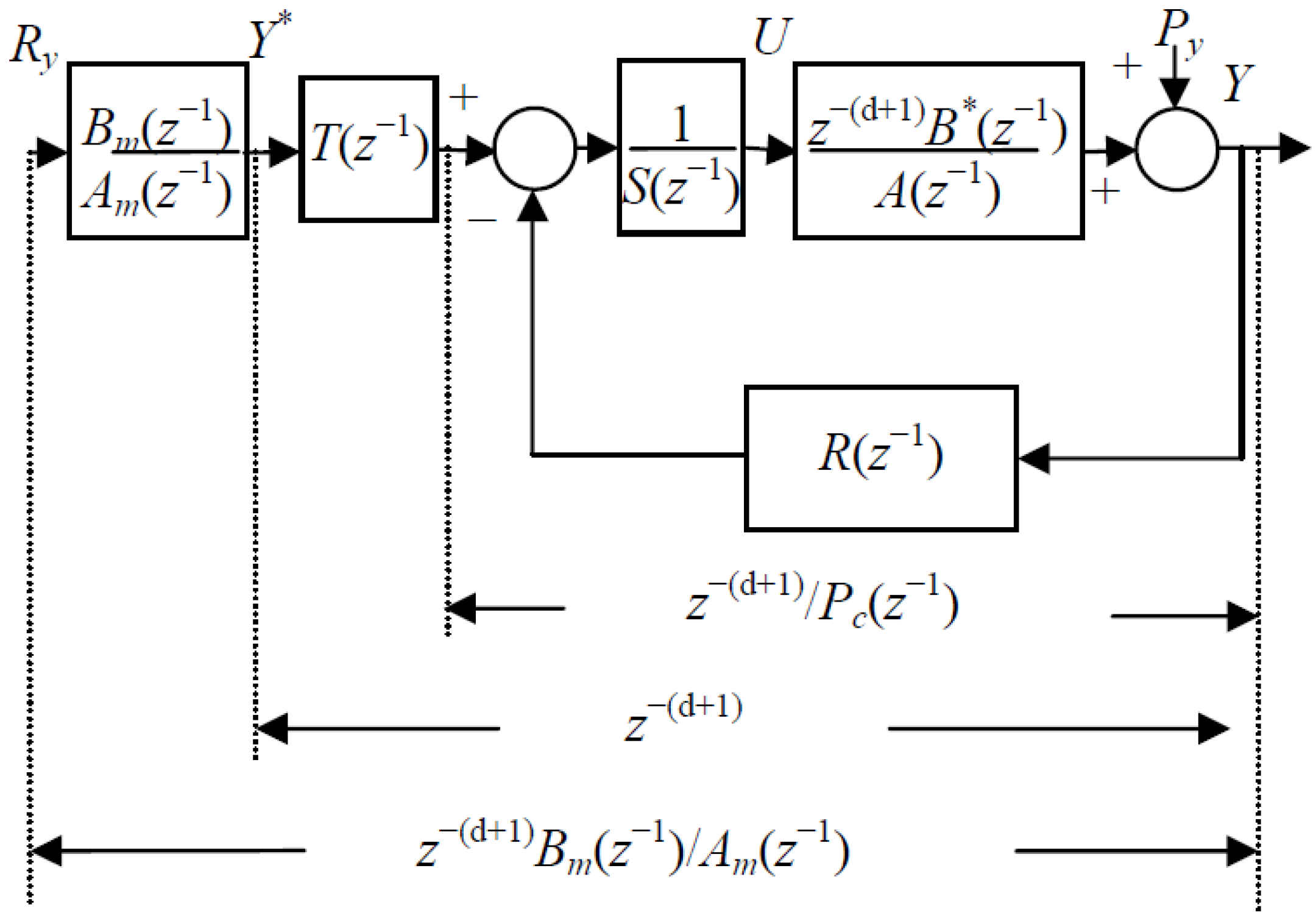
3.1.3. “Tracking and Regulation with Independent Objectives with Sensitivity Function Shaping” Method

The method contains two different steps [16]. Firstly, the controller is designed in order to adjust the desired behavior in regulation through R and S polynomials (see Figure 5). Secondly, the tracking behavior is adjusted through T, A_m and B_m. polynomials. In Figure 5, A and B (B^* without the digitizing delay) represent respectively the denominator and the numerator of the plant. d is the delay expressed in number of samplings (here d = 0). Concerning the different signals, Y is the output of the plant, Y^* the output reference, U the control signal, P_y the disturbance applied to the output of the plant and R_y the reference signal before the reference model which is defined by A_m and B_m polynomials. Finally, P_c is the characteristic polynomial of the CL system.

Figure 5. Block-diagram of a RST digital controller.

Figure 5. Block-diagram of a RST digital controller.

With respect to the behavior in regulation, knowing the plant model (A, B and d) and the desired specifications (P_{c_des}), the expression of R and S polynomials have to be found in order to fulfill the following relation:

P_c = A(z⁻¹)S(z⁻¹) + z^−(d+1) B^* (z⁻¹)R(z⁻¹) = P_{c_des}

(12)

Pre-specifications can be introduced through S and R polynomials. Thus, generally, these polynomials are written as follows:

S (z⁻¹) = H_S (z⁻¹)S'(z⁻¹) and R (z⁻¹) = H_R (z⁻¹)R'(z⁻¹)

(13)

For instance, to obtain a zero static error in response to a step, as the plant has no integrator, one must be introduced in the controller. This is obtained taking:

H_s (z⁻¹) = (1 − z⁻¹)

(14)

The desired characteristic polynomial P_{c_des} contains dominant poles included in P_d and auxiliary fast poles (non-dominants) included in P_f polynomial. Moreover, in this method, in order to cancel out the plant transfer function numerator, B^* is included in P_{c_des}:

P_{c_des} (z⁻¹) = P_d (z⁻¹)P_f (z⁻¹)B^* (z⁻¹)

(15)

This way, as it can be seen in Equation (15), the resolution of this equation leads to the presence of B^* in S, and consequently, to its canceling out (the canceling out of B^* can also be carried out introducing it in H_S, instead of P_c, and thus simplifying Equation (12) [16]).

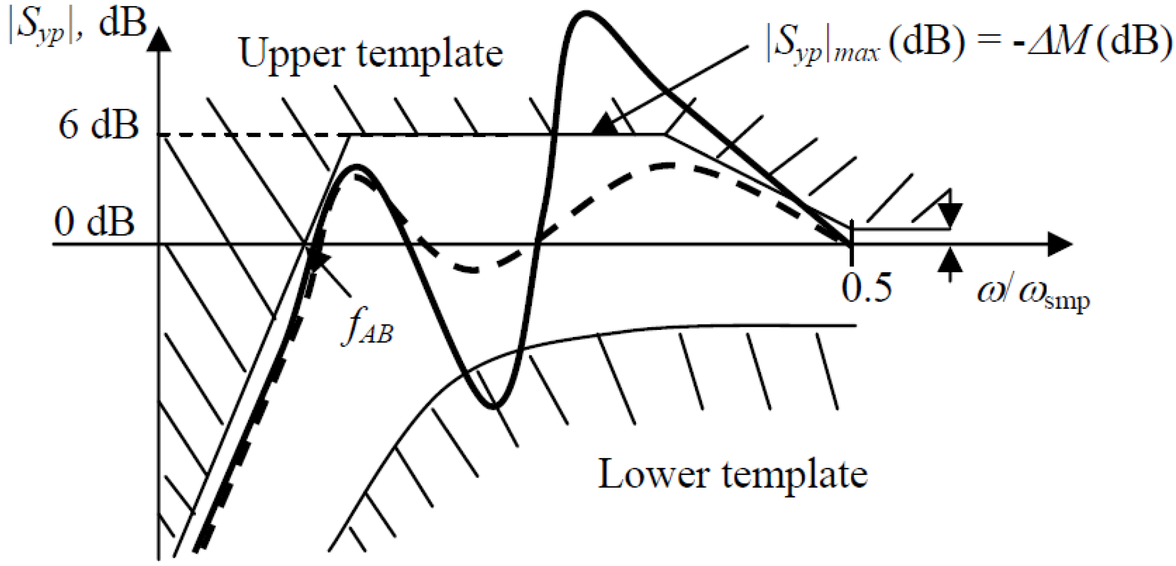
Pre-specifications of S and R polynomials, as well as P_f polynomial can be also used to adjust the robustness of the controller. The modulus and delay margins, ∆M and ∆τ, are better robustness indicators than gain and phase margins [16]. The modulus margin is related to the maximum gain of the sensibility function S_yp between the output disturbance and the output. The delay margin is also linked to this transfer function. Thus, robustness specifications are generally set defining a template for the Bode magnitude diagram of S_yp, as shown in Figure 6.

Figure 6. Template of the Bode magnitude diagram of the sensitivity function S_yp.

Figure 6. Template of the Bode magnitude diagram of the sensitivity function S_yp.

The maximum of S_yp must be lower than 6 dB. This fulfillment ensures a modulus margin higher than −6 dB. Moreover, the magnitude of S_yp has to be rather close to 0 dB in high frequencies in order to ensure a delay margin higher than a sampling period [16]. This template allows also specifying the speed of the system behavior in regulation, through the adjustment of the attenuation band frequency f_AB.

One property of the sensitivity function says that “for asymptotically stable CL, and stable open loop, the integral of the logarithm of the modulus of the sensitivity function S_yp form 0 to 0.5 f_s is zero”. This means that if changing the controller parameters the gain of S_yp increases in some frequencies, it decrease in other ones. For that reason, a lower template is also defined for S_yp, as can be seen in Figure 6. The tuning of the controller in order to fulfill the specifications consists in adjusting the Bode magnitude diagram of S_yp through H_S, H_R and P_{c_des}, in order to enter it in the defined template. Regarding the tracking behavior design, in this method, T is used to cancel out the regulation dynamics (Figure 5), taking T = P_c = P_dP_f. Once the regulation dynamics are canceled out, the tracking dynamics is tuned through A_m and B_m polynomials related to the reference model.

3.1.4. Robust Controller Design and Adjustment

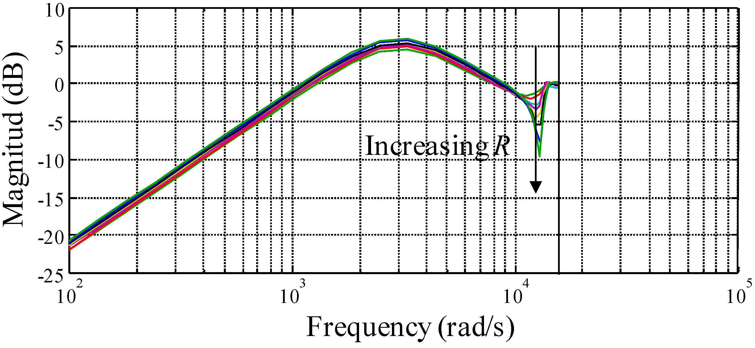
In a first step, the desired dominant poles included in P_d are specified with a damping factor ξ = 0.7 and a settling time t_s (5%) = 1 ms. Moreover, in order to fulfill the specification related to the static behavior, an integrator is included in H_S. The other polynomials (H_R and P_f) are taken equal to 1. Figure 7 shows the obtained S_yp Bode magnitude diagram.

The obtained modulus margin is too low (∆M = −11.88 dB). It is also observed that the gain is very small in high frequencies. Thus, two slightly damped auxiliary poles (ξ = 0.16) are introduced in high frequencies (ω_n = 1.45 × 10⁴ rad/s), increasing the gain in high frequencies and thus decreasing the gain in medium frequencies and raising the modulus margin. With this new tuning, the robustness margin takes the following values: ∆M = −4.42 dB and ∆τ = 3.94 T_s (see also Figure 7).

Figure 7. Bode magnitude diagram of S_yp of the Robust current controller at different operating points.

Figure 7. Bode magnitude diagram of S_yp of the Robust current controller at different operating points.

The adjustment of the controller being appropriate, the aforementioned second condition related to the sampling time can be verified. With the tuned speed, the sampling frequency is 10 times higher than the desired CL bandwidth. Thus, the second condition is fulfilled.

A study of the CL system in regulation in the other operating points is carried out. Figure 7 shows, as it was supposed, that the attenuation band is lower when the resistance increases, while the robustness margins are higher. Thus, this way, the stability and robustness in stability are ensured in the whole operating zone. Regarding the tracking dynamics, the reference model is chosen as a first order with unitary static gain and a settling time of t_s (5%) = 1 ms.

3.1.5. Gain Scheduling Controller Design

Different kinds of GS strategies exist [17]. The first types of methods are based on a Linear Parameter-Varying description of the plant. They ensure global properties of the CL system. The second class of methods consists in computing a set of local controllers on a bank of linearized models. This second method provides control systems which only ensure local properties. Consequently, global stability and global performance have to be checked a posteriori, generally through simulations.

In this study the used method has been the second type one. Considering the study carried out in Section 2.3, the load resistance is chosen as scheduling parameter. It is estimated through filtered current and voltage measures at the inverter filter output.

Nine operating points are considered, those corresponding to R_nom, 1.5 R_nom, 2 R_nom, 3 R_nom, 4 R_nom, 5 R_nom, 6 R_nom, 8 R_nom and 10 R_nom. The scheduling regions are delimited in function of these points. For the identification of the scheduling region, a hysteresis filter is applied to the estimated load in order to avoid unnecessary switching.

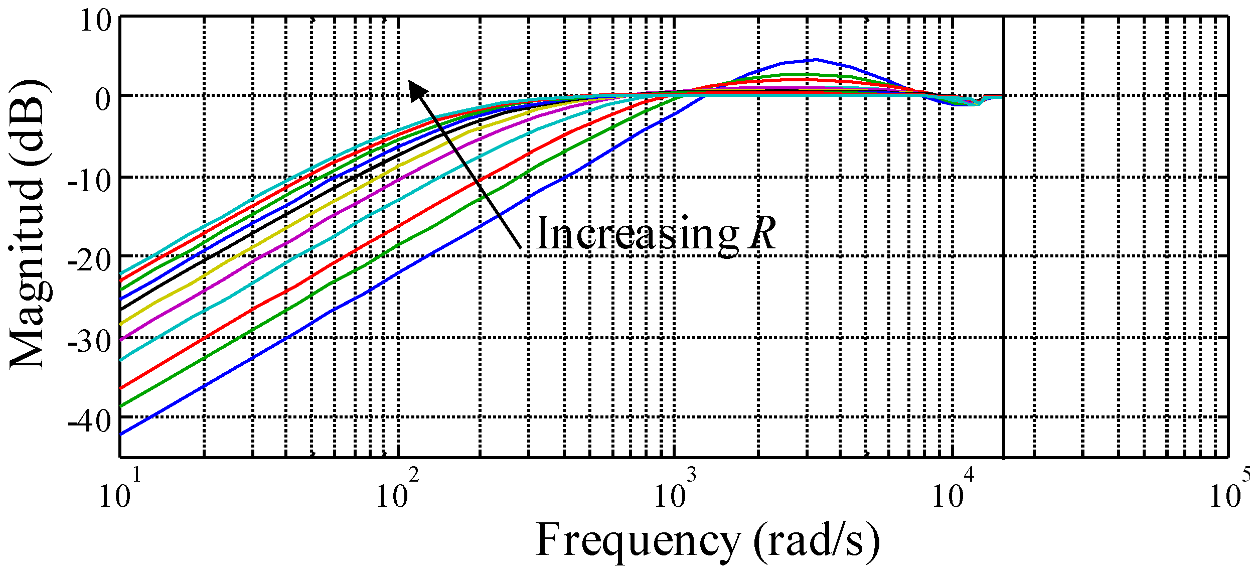
A controller is designed for each considered operating point following the same aforementioned methodology, through the digital control model obtained in each operating point. The specifications are the same as those of the Robust controller. Only P_f polynomial is changed in order to obtain the best robustness margins in each operating point. Figure 8 shows the Bode magnitude diagram of S_yp obtained with each controller. The modulus margin is always between −4.59 and −5.84 dB. Regarding the delay margin, it is higher than T_s for all controllers. Figure 8 shows also that f_AB is similar for all controllers, contrary to what it is observed in Figure 7 for the Robust controller. The switching between different controllers is carried out with a bumpless strategy.

Figure 8. Bode magnitude diagram of S_yp of the current GS controller at different operating points.

Figure 8. Bode magnitude diagram of S_yp of the current GS controller at different operating points.

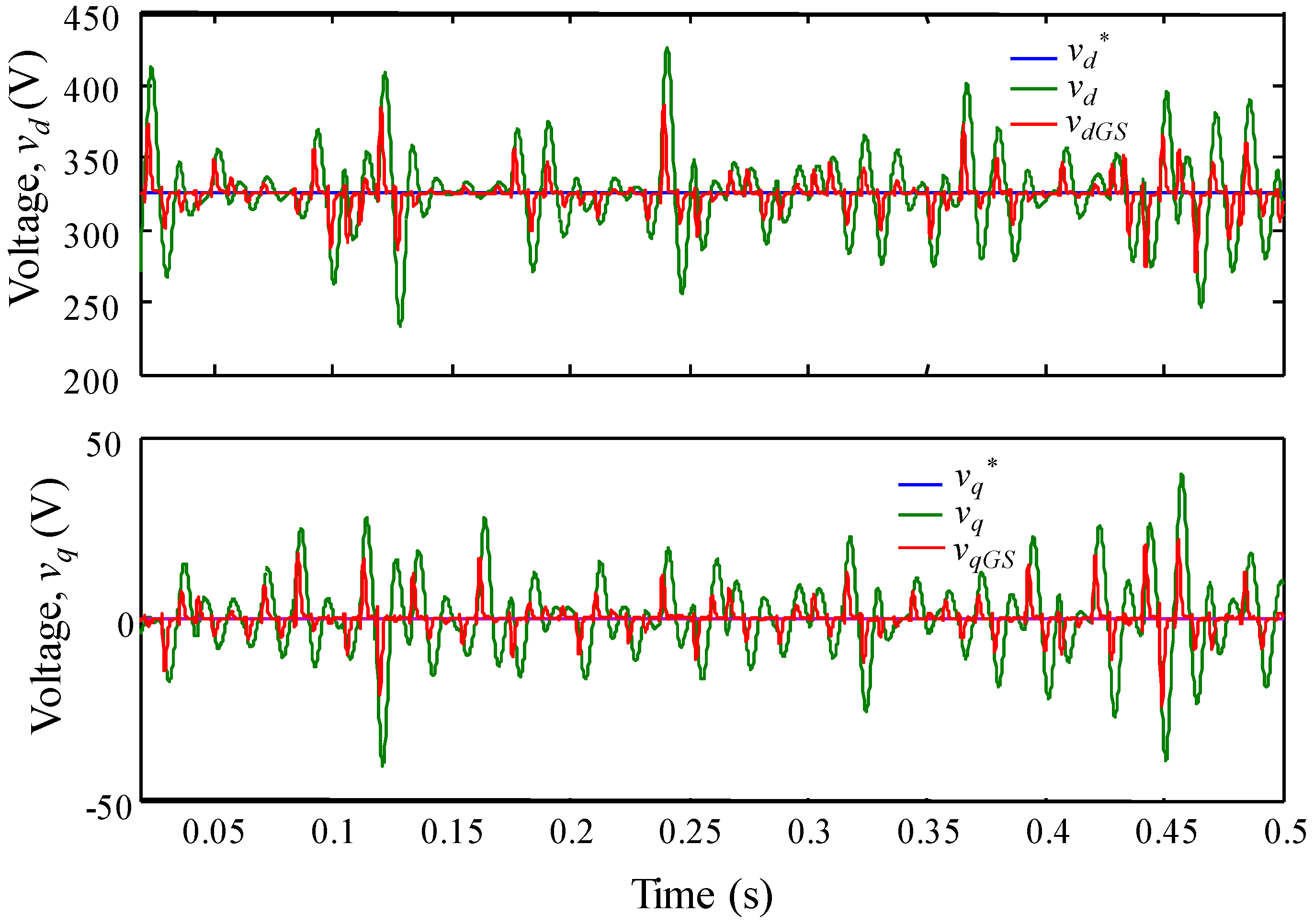
3.2. Voltage Loop

For this outer loop, as for the current loop, two different controllers are designed: a robust one and a GS type one. The plant is still nonlinear here. Postulating that the current controller has been appropriately designed, the plant model is composed by the product of the inner loop reference model and the resistance value R. Thus, as for the plant of the current loop, the nonlinearity is related to the resistive load value.

3.2.1. Control Objectives

The objective of the voltage controller is to regulate v_d and v_q voltages through the current references in d and q reference axes i_d^* and i_q^*. Moreover, as for the current loop, the Robust controller has to be stable and robust in stability in the whole operating zone, with the same robustness margins defined previously. Concerning the specifications related to the static behavior, the response to a step of reference and disturbance should be zero. Regarding the GS controller, on top of these specifications, it has to keep the same CL system settling time in the whole operating zone.

3.2.2. Control Model

As mentioned above, the control model is composed by the product of the inner loop reference model and the resistance value R:

(16)

The desired settling time for the voltage loop being the same as that of the current loop, the chosen sampling time is also the same. For the Robust controller, the nominal operating point has to be chosen. From Equation (16), it can be easily seen that the gain of the transfer function is proportional to R. Thus, the maximum gain is obtained for the maximum value of R, it is to say the operating point corresponding to the lowest power consumption. If the Robust controller is designed through the control model corresponding to this operating point, the controller should be robust in the rest of the operating zone where the gain of the plant is lower. Regarding the CL behavior, it will be slower when R decreases.

The obtained control model in the selected nominal operating point (R = 10 R_nom) is:

(17)

This transfer function does not contain zeros. The “Pole placement with sensitivity function calibration” method is used to design the voltage controllers [16]. It is very similar to the previous method. The only difference is that the plant numerator is not canceled out (B^* is not included in P_{c_des}).

3.2.3. Robust Controller Design

The obtained controller is relatively simple. An integrator is included in H_s. Moreover, the desired CL polynomial characteristic is that of the current loop reference model, A_m. Thus, the used controller design method is equivalent to the “Internal Model Control”. Concerning the P_f polynomial, it is taken equal to 1. H_R is used to fix S_yp gain to 0 dB in 0.5 f_s in order to ensure a good delay margin. The obtained robustness margins are: ∆M = −3.9 dB and ∆τ = 2.23 T_s. 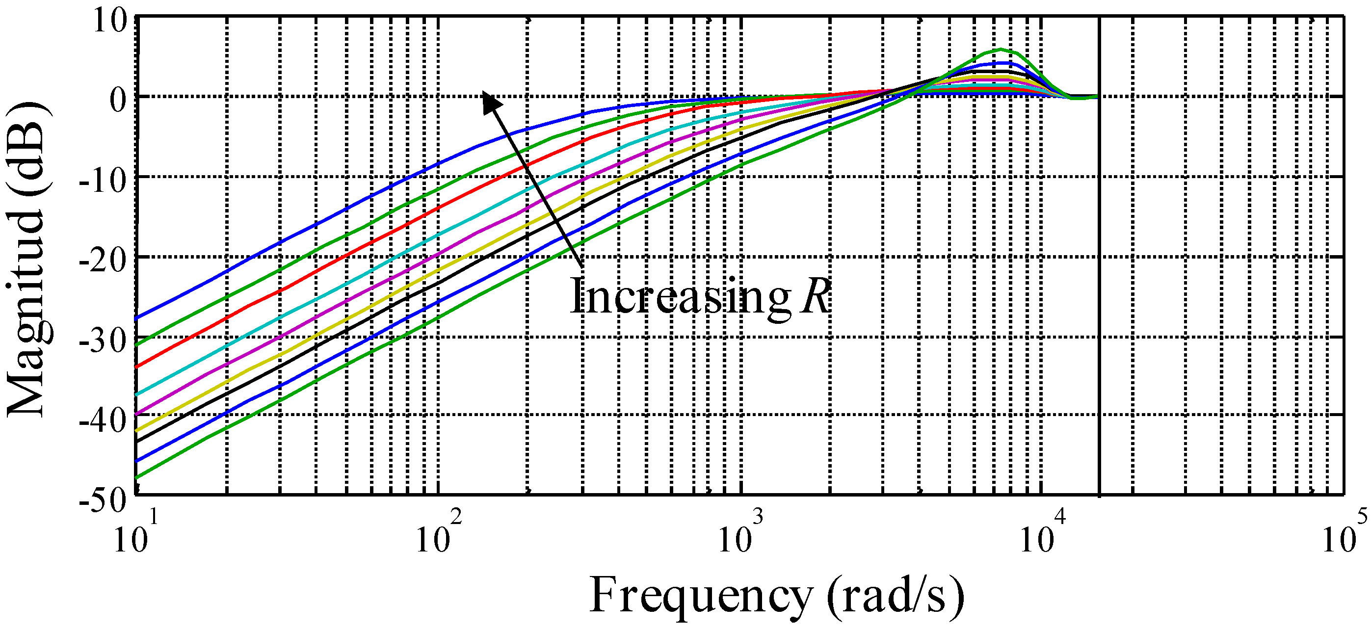Figure 9 shows the Bode magnitude diagram of the sensitivity function for this controller in different operating points. As predicted before, the robustness margins obtained for lower value of R are higher than those corresponding to the nominal point R = 10 R_nom, while f_AB is lower.

Figure 9. Bode magnitude diagram of S_yp of the Robust voltage controller at different operating points.

Figure 9. Bode magnitude diagram of S_yp of the Robust voltage controller at different operating points.

Regarding the tracking dynamics, it is not so important because the voltage set-points in d and q reference axes are constant:

(18)

T is used to cancel out the regulation dynamics and ensure a unitary static gain. For the startup dynamics, a first order reference model with a settling time t_s (5%) = 1.5 ms and unitary static gain is considered.

3.2.4. Gain Scheduling Controller Design

The GS controller is designed following the same process as for the current loop. The same scheduling parameter (estimated and filtered in the same way) and scheduling regions are considered. The controllers in the different points are designed and tuned with the same specifications as the Robust controller of the voltage loop. The obtained S_yp and robustness margins for all local controllers are the same as those of the Robust controller in the nominal operating point: ∆M = −3.9 dB and ∆τ = 2.23 T_s.

4. Simulation Results and Discussion

Simulations have been carried out through a simulation model which takes into account the inverter commutations and the duty cycle limits. In the next Section, simulations results related to the study of the two current controllers in regulation and tracking modes are presented and discussed. The voltage controllers are compared in Section 4.2.

4.1. Current Loop Simulation

In a first simulation trial the current loop regulation behavior is analyzed changing the value of R each 0.1 s to these values: R_nom, 2 R_nom, 4 R_nom, 6 R_nom, 8 R_nom. When R increases, the current decreases instantly, generating a disturbance in the output of the plant. Furthermore, when R changes the operating point (and thus the plant dynamics) changes also.

Figure 10 shows the response of i_d to R variations. The current reference is constant, at 0.5 A. It can be seen that the plant is well damped in CL with both controllers. When R increases, as predicted, the settling time of the Robust controller also increases, while that of the GS controller remains constant. For high values of R, the difference between the two controllers is important. Indeed, the settling time is of 2 ms with the GS controller while it is of 17.5 ms with the Robust controller.

In the same way, Figure 11 shows the response of i_q when R changes as before and i_q set-point is 0 A. Slight transient oscillations at the plant resonant frequency appear when R value changes. However, their amplitude is quite low and the transient is short. When increasing i_q set-point, oscillations are not noticed, as with i_d. A second simulation test is accomplished in order to analyze the tracking behavior of the inner loop. The test is carried out with the two controllers in two different operating points. In t = 0.1 s, i_d set-point changes from 0.25 to 0.5 A, and in t = 0.15 s, the set-point value returns to 0.25 A.

Figure 12 shows the response of i_d current to these set-point changes for the two controllers in the two extreme operating points, R = R_nom and R = 10 R_nom. The response obtained with the GS controller is the same in the two operating points. Moreover, it is the same response as that obtained with the Robust controller when R = R_nom. Regarding the CL behavior with the Robust controller when R = 10 R_nom, the settling time is significantly higher than that of the previous cases, 22 ms vs. 1 ms. Thus, regarding the current loop, the carried out simulation trials shows that, unlike the Robust controller, the GS controller allows ensuring the same dynamical behavior in the whole operating zone.

Figure 10. Temporal response of i_d in regulation, for the two controllers, when R changes each 0.1 s taking these values: R_nom, 2 R_nom, 4 R_nom, 6 R_nom, 8 R_nom.

Figure 10. Temporal response of i_d in regulation, for the two controllers, when R changes each 0.1 s taking these values: R_nom, 2 R_nom, 4 R_nom, 6 R_nom, 8 R_nom.

Figure 11. Temporal response of i_q in regulation, for the two controllers, when R changes each 0.1 s taking these values: R_nom, 2 R_nom, 4 R_nom, 6 R_nom, 8 R_nom.

Figure 11. Temporal response of i_q in regulation, for the two controllers, when R changes each 0.1 s taking these values: R_nom, 2 R_nom, 4 R_nom, 6 R_nom, 8 R_nom.

Figure 12. Temporal response of i_d when the current reference changes in t = 0.1 s from 0.25 to 0.5 A, and in t = 0.15 s from 0.5 to 0.25 A for both controllers in two different operating points, R = R_nom and R = 10 R_nom.

Figure 12. Temporal response of i_d when the current reference changes in t = 0.1 s from 0.25 to 0.5 A, and in t = 0.15 s from 0.5 to 0.25 A for both controllers in two different operating points, R = R_nom and R = 10 R_nom.

4.2. Voltage Loop Simulation

Once the good working of the inner loop has been checked, the voltage loop operation is tested in regulation mode. Indeed, the voltage set-points are kept to constant values (v_d^* = 325 V and v_q^* = 0 V) and a disturbing current related to burst types fast active and reactive power variations [15] is modeled and injected into the plant output, as depicted in Figure 1. The total consumed current related to the resistive loads and FVLs corresponds to an operating point around 6 R_nom.

Figure 13 shows this three-phase disturbing current. It can be observed that the sinusoidal signals are distorted, with fast varying amplitudes.

Figure 13. Disturbing three-phase current related to fast active and reactive power variations.

Figure 13. Disturbing three-phase current related to fast active and reactive power variations.

Figure 14 shows the response obtained for v_d and v_q voltages for the two types of controllers. The CL behavior is better with the GS controller (v_dGS and v_qGS voltages).

Figure 14. Voltage time series obtained with the two different controllers in the presence of a current disturbance corresponding to FVL.

Figure 14. Voltage time series obtained with the two different controllers in the presence of a current disturbance corresponding to FVL.

Indeed, thanks to the higher dynamics of this controller around the operating point, the disturbances are most quickly rejected. A similar behavior is observed for v_d and v_q. Figure 15 and Figure 16 confirm these results. In both figures, it can be noted how the tracking of the current references generated by the voltage loop is tighter with the GS controller. The d and q axes currents are virtually superposed to their references with the GS controller, while with the Robust controller, the tracking is slower.

Figure 15. d axis current obtained with the two different controllers in the presence of a current disturbance corresponding to FVLs.

Figure 15. d axis current obtained with the two different controllers in the presence of a current disturbance corresponding to FVLs.

Figure 16. q axis current obtained with the two different controllers in the presence of a current disturbance corresponding to FVLs.

Figure 16. q axis current obtained with the two different controllers in the presence of a current disturbance corresponding to FVLs.

Figure 17 shows the three-phase voltage obtained at the inverter filter output with the two different controllers during the same simulation test. With the Robust controller, the amplitude of the three sinusoids varies, while it is virtually constant with the GS controller. Only some rare variations related to the most severe disturbances are visible with this controller.

Figure 17. Three-phase voltage obtained at the inverter filter output with the two different controllers in the presence of a current disturbance corresponding to FVLs.

Figure 17. Three-phase voltage obtained at the inverter filter output with the two different controllers in the presence of a current disturbance corresponding to FVLs.

The total harmonic distortion (THD) of the first phase signal obtained with the two controllers is measured thanks to the related SimPowerSystems toolbox block of Simulink. The THD obtained with the Robust controller if 8%, while that obtained with the GS controller is 1.9%.

Finally, Figure 18 shows the produced active power for the same scenario as that of the previous Figures. It can be verified that the power variations are severe in general and of the burst type [15]. Moreover, it can be seen that produced power variations are slightly filtered with the GS controller.

Figure 18. Active power produced by the inverter with the two different controllers in the presence of a current disturbance corresponding to FVLs.

Figure 18. Active power produced by the inverter with the two different controllers in the presence of a current disturbance corresponding to FVLs.

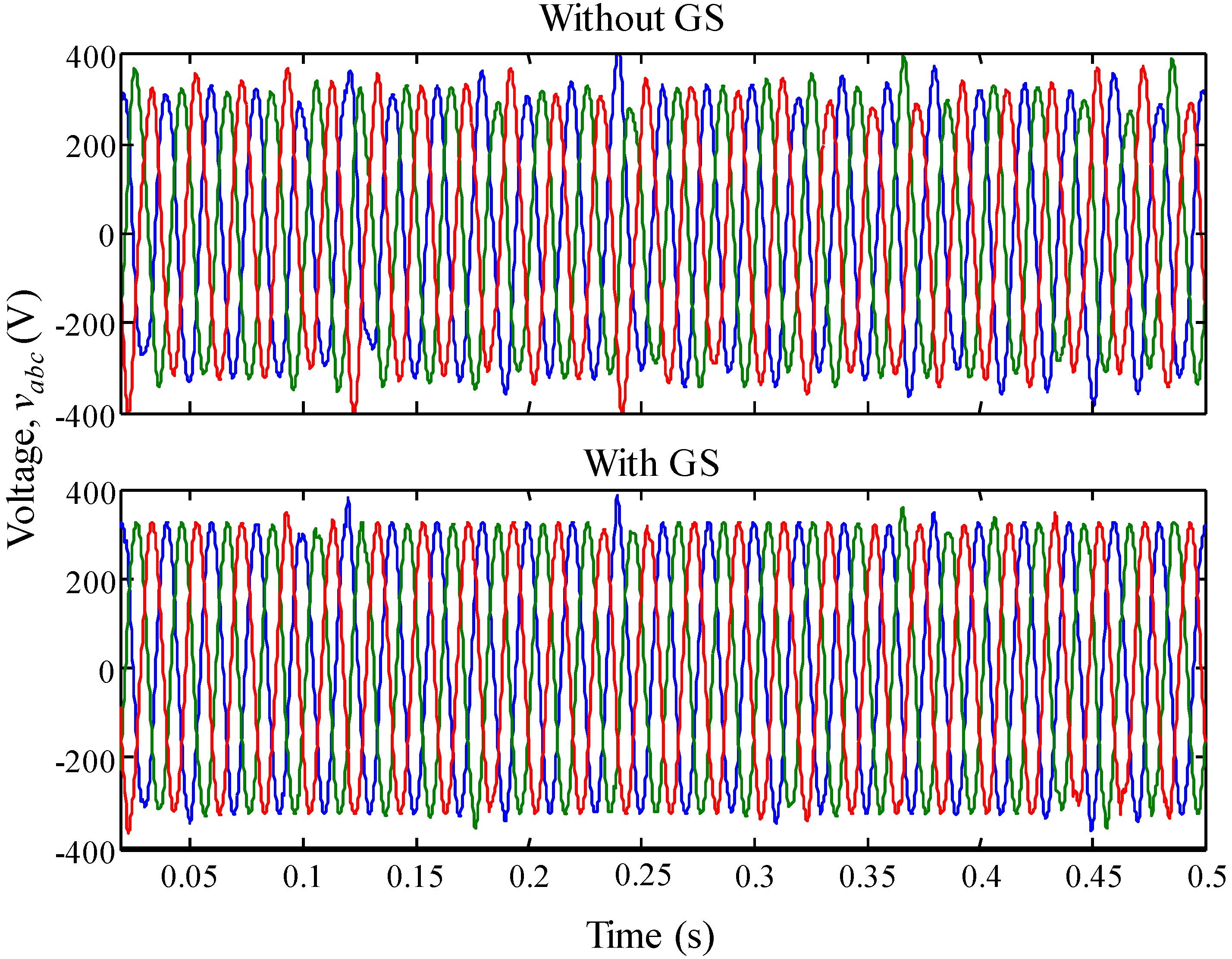
5. Conclusions and Perspectives

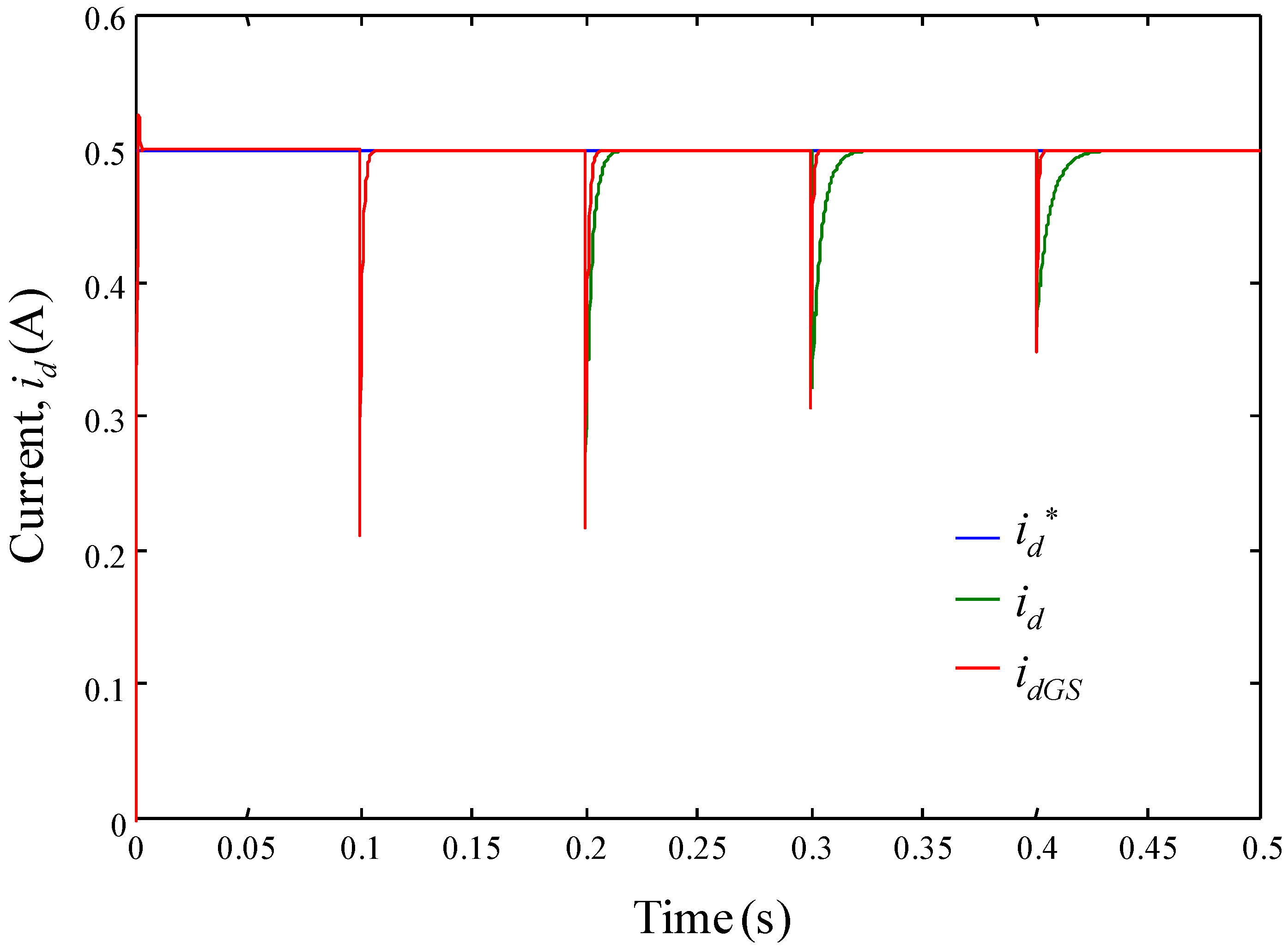
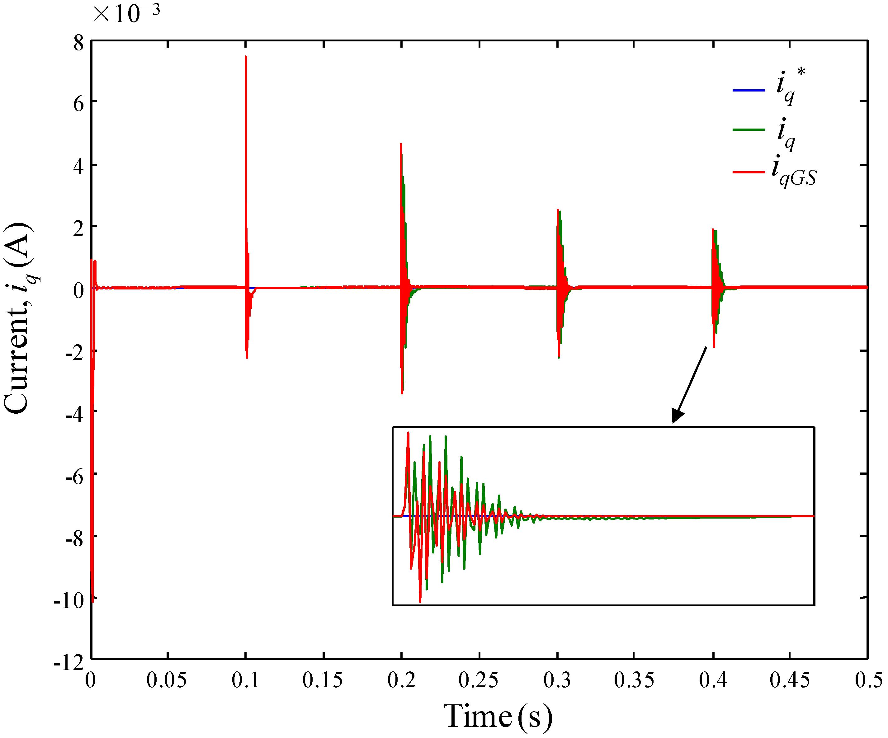
As predicted in the design of the controllers, unlike the Robust controller, the GS controller allows ensuring the same dynamical behavior in the whole operating zone. The design of the Robust controller is conservative because its main objective is to ensure the fulfillment of the specified robustness margins in the entire nonlinear operating zone. For this controller, the operating zone related to low values of consumed power (or high values of the load) is a bit problematic, because there, the inner loop dynamics is relatively slow. Moreover, in this case, the inner loop is slower than the outer one. Anyway, it has been proved that both controllers damp the oscillatory behavior of the plant and that they reject output disturbances relatively quickly. But, in presence of FVL, the THD produced with the Robust controller could be excessive, while it is acceptable with the GS controller.

Regarding the controllers’ robustness, the stability has been ensured in all carried out tests. Moreover, the GS controller is also robust in performance. However, as with this GS strategy the global stability is not guaranteed analytically, more trials should be carried out in order to test it. That is one of our perspectives, to make more tests in order to ensure the stability robustness of the GS controller, as explained in [17]. Furthermore, experimental trials (including robustness tests) are planned in the EneR-GEA experimental microgrid [14]. Moreover, for the design of the controllers which will be tested in that platform, it is foreseen to obtain the different control models corresponding to the considered operating points by identification, and to decrease the GS regions number considered here, in order to reduce the computational time.