Pitch Based Wind Turbine Intelligent Speed Setpoint Adjustment Algorithms


Abstract
: This work is aimed at optimizing the wind turbine rotor speed setpoint algorithm. Several intelligent adjustment strategies have been investigated in order to improve a reward function that takes into account the power captured from the wind and the turbine speed error. After different approaches including Reinforcement Learning, the best results were obtained using a Particle Swarm Optimization (PSO)-based wind turbine speed setpoint algorithm. A reward improvement of up to 10.67% has been achieved using PSO compared to a constant approach and 0.48% compared to a conventional approach. We conclude that the pitch angle is the most adequate input variable for the turbine speed setpoint algorithm compared to others such as rotor speed, or rotor angular acceleration.
1. Introduction
This paper presents the application of intelligent optimization techniques in wind turbine rotor speed setpoint control algorithms. Setpoint algorithms are compared in order to achieve two main objectives: to capture as much mean power as possible and to avoid reaching the tower resonance, which involves security stops with the corresponding mechanical fatigue and efficiency loss.
The rotor speed setpoint is highly related to power generation dispatch algorithms. In our case, a 100 kW Wind Turbine, the control must capture as much power as possible, but in other wind turbine systems such as [1], a probabilistic approach is taken in power generation dispatch. Rotor speed setpoint algorithms are compared in different wind regimes. The simplest reference algorithm maintains a constant setpoint. The alternative conventional algorithm tries to capture as much mean power as possible. This algorithm is the most popular one as it does not need very complex information or calculations. However, it does not take into account possible over speeds due to high rotor speed setpoints.
In a first approach we have applied a Reinforcement Learning (RL) scheme. In wind turbine control, the most important variable is wind speed. This variable has stochastic behaviour, as the environment is changing all the time. In consequence, when the RL algorithm is applied to a stochastic dynamic, we must model the problem as a Markov Decision Process (MDP). MDP is a framework for optimal system control modelling in uncertain dynamic environments. MDP was first studied by Bellman [2]. Since then MDP has been extensively used to study and embody RL systems.
There are different works on RL-MDP applied to wind turbines [3,4], but they use RL in wind turbine maintenance polices. Other authors apply RL algorithms to rotor speed control loops as in [5]. The latter papers propose a complex algorithm to adapt the pitch based rotor speed control gains. In our case, the RL-MDP framework is applied to improve the rotor speed setpoint algorithm.
An MDP framework is defined by states, actions and probability of transition from one state to another. MDP states may be continue or discrete. In [6–9] for example, an RL scheme is proposed in a multi body linked system control. Usually, in this kind of problems the states are quantified in many level or possible values.
After multiple experiments, the choice of the proposed RL scheme was rejected, because it does not improve the conventional algorithm results. This question is further detailed later. As an alternative intelligent algorithm a Particle Swarm Optimization (PSO) based adjustment scheme is proposed. PSO is a bio-inspired computational technique based on the idea of natural swarm learning mechanisms, where living organisms remember successful positions of the swarm and use them to improve future rewards. This algorithm has been applied in Wind Turbine design with success [10].
The paper is organized as follows: Section 2 establishes the problem statement. Section 3 describes the wind turbine model: aerodynamics, power train and electrical machine. Wind regimes are explained in Section 4. Section 5 describes the conventional algorithm. Section 6 is devoted to the first proposed control system based on Reinforcement Learning. Section 7 is dedicated to the second proposed control algorithm based on Particle Swarm Optimization. Section 8 provides results and comparison. Finally, the paper is concluded in Section 9.
2. Problem Statement
Wind turbine control algorithms adjust the setpoint in order to capture as much mean power as possible while preventing from reaching the tower resonance speed. These two objectives are achieved maximizing a reward function which is bounded between zero and one. This function is defined as the product between two sigmoid function form terms.
It is important to capture as much mean power as possible but, for example, if the control surpasses a certain power limit, the reward saturates. This effect has been taken into account in the first term of the reward function. The second term is related to rotor speed. A low rotor speed is a consequence of low wind speed. However this term is more relevant when the rotor speed increases up to the setpoint speed. Above this speed the corresponding term saturates. This reward function is described in Section 6.1.
3. Wind Turbine Modelling
The wind turbine plant is described by a classical model. The most important parts of the model are the power train, the power stage, the blades' aerodynamics and the electrical machine.
3.1. Wind Turbine Aerodynamics
When an airfoil moves through a fluid, it supports three types of stress: lift, drag and pitch moment. Specifically the lift is responsible for turning the turbine and its azimuthal torque. However, from the Control Engineer's point of view, the parameter that best defines the wind turbine behaviour is the power coefficient. This coefficient indicates the percentage of kinetic energy of the passing air captured by the wind turbine per time unit.
In fact, it is common to express the aerodynamics torque Tw in the following way [11]:
Pw: wind turbine power;
w: wind turbine angular speed;
ρ: air density;
Cp: aerodynamic power coefficient;
vw: wind speed;
R: rotor blade radius.
Manufacturers usually provide the aerodynamic power coefficient Cp as a function of the tip speed ratio λ and the pitch angle β. The tip speed ratio λ is the relation between rotational speed of the tip of a blade w·R and the velocity of the wind vw. It is defined by:
There exist many other more complex models that may be consulted in [12–14]. These models describe the dynamic interactions among the control variables such as the pitch and the yaw angles, and the different stresses and moments over the nacelle and the tower. On the other hand, models based on computational fluid dynamics can be used for more detailed and physically reliable calculations but due to the huge computational time required these methods are not useful in control experiments.
In pitch control the most interesting variables are the flapping and bending moments at the blade roots, together with the gyroscopic effects such as the furling forces. All these effects are described in [12] and they are modelled both in Matlab/Simulink [15] and in FAST [12,16].
The tower and the nacelle dynamics are modelled by finite element techniques given by CAD platforms (for example Catia). When these dynamics are taken into account in control algorithms design, NREL software platforms are frequently used, mostly FAST [12,16]. Furthermore, when the control algorithm has to take into account the tower and nacelle dynamics, the foundation must also be modelled.
3.2. Power Train Model
The dynamics of the power train model is one of easiest part to be described, apart from the torsion elasticity effects. The torsion elasticity is mainly defined by the elastic link of commercial elements and their technical characteristics are often not well known. Another frequent problem is the gear losses dynamics. In fact, these losses change the curve torque vs. rotor speed when the turbine is operating in a maximal power coefficient mode. This question, together with the electrical machine, is very important as the power stage strongly influences the wind turbine performance:
Tw: aerodynamic torque seen from the turbine axis;
Tem: electrical machine torque seen from the turbine axis;
c: power train damping coefficient;
Jtot: total inertia defined by Equation (4).
Jturbine: wind turbine inertia;
Jgenerator: electrical machine inertia;
igear: gear reduction ratio.
3.3. Electrical Machine and Power Train Model
100 kW wind turbine generators usually have full converter asynchronous machine topologies. The main reasons for that are the cost of power electronics, the cost of electrical machine and the power performance behaviour vs. rotor speed. The drawback of this topology is the need of a gear because it increases the weight and the cost of the power train. Synchronous electrical machines with external excitation are unusual not only due to their high required maintenance but also for their excessive cost, which is only justifiable for high power installations (1 MW) [17]. In this power range, these machines are replaced by double fed asynchronous machines for their cheaper power stages [17].
The permanent magnet machines are utilized in medium and high power wind turbines without gear. This characteristic makes these wind turbines cheaper with higher performance. In order to make compatible the speed spread of the electrical machine and the speed spread of the wind turbine a gear is set in the power train.
The main criteria to select the electrical machine for a wind turbine are:
Economical cost of the electrical machine: Permanent magnet machines are the most expensive as they are built with rare earth elements. In contrast, asynchronous machines are the cheapest, with a typical price ratio of about two or three. Commuted reluctance synchronous machines are pricewise in between the two previous models;
Economical cost of the power stage: The price of power stages depends on the power they must manage. The complexity of the electrical machine control is another factor that increases the price of the power stage. Double fed asynchronous power stages are the cheapest as they handle four times less power;
Performance vs. speed spread: Performance at rated speed is a very important factor, but it usually decreases as the rotor speed decreases. In permanent magnet machines performance is reduced less than in asynchronous machines with a rotor speed below the rated speed. In asynchronous machines full converter topologies performance decreases more than for other electrical machines when the rotor speed is under the rated speed;
Electrical machine volume and mainly its weight: The volume of the electrical machine is another important factor because it imposes strong mechanical design restrictions. It determines other control subsystems such as the pitch actuator. On the other hand, the electrical machine weight produces a reduction of the forwards-backwards tower resonance frequency;
The need for a gear in the power train: Some machines do not need a gear, with the corresponding cost reduction. Besides, the performance increases, and the tower forwards-backwards resonance frequency increases. In our case, an asynchronous full converter topology has been chosen because of its cheapest price, even though they need a gear and show worse performance at low speeds.
The power stage has been modelled by a first order system. The input is the torque demand; the output is the real torque given by the electrical machine. A τps time constant has been identified after several trials made with the power stage:
: aerodynamic torque demand or setpoint seen from the turbine axis;
τps: The power stage's torque loop time constant.
This equation only models the torque dynamics because our objective is not to develop the power stage control.
4. Wind Speed Model
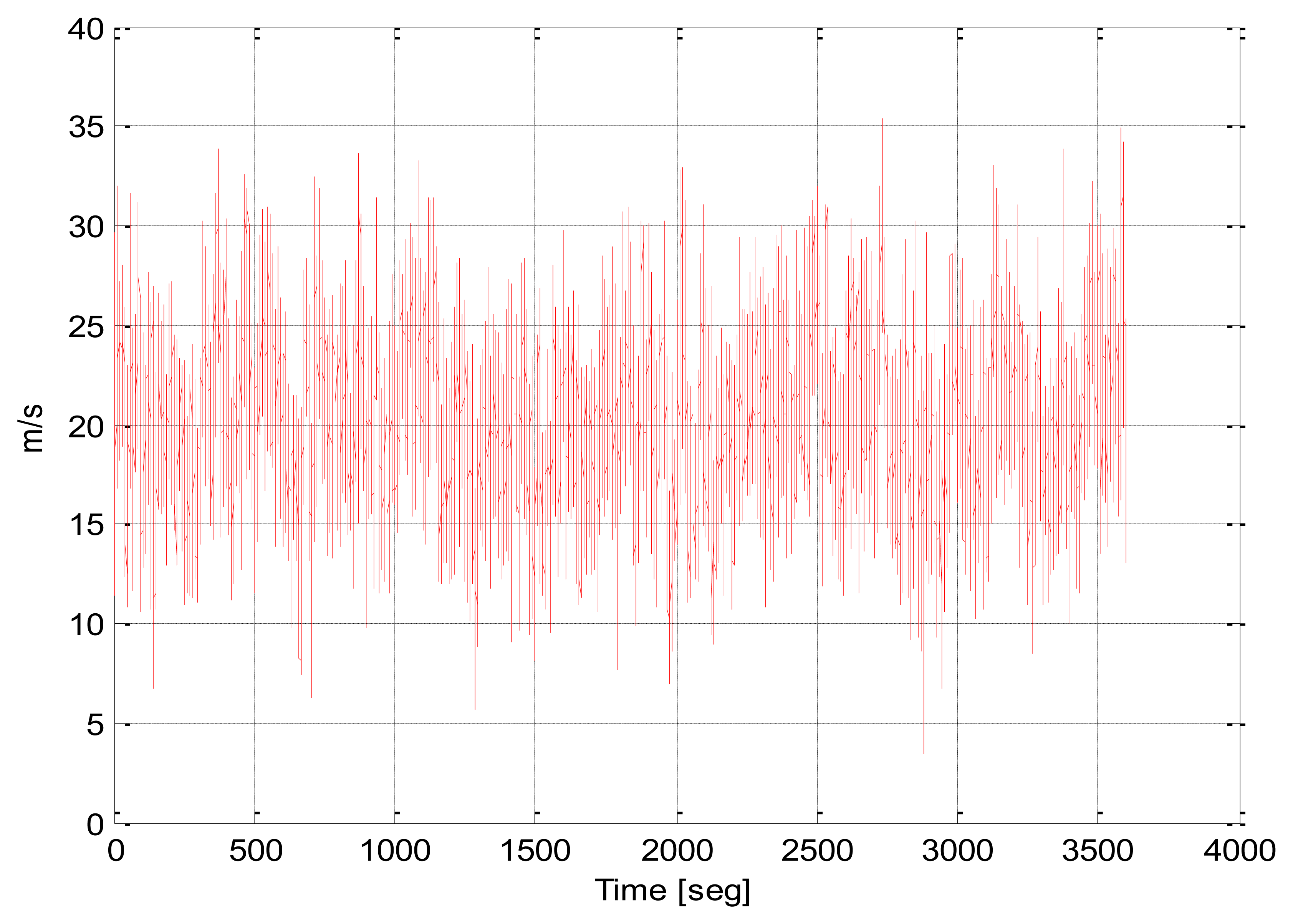
The wind speed realizations utilized in our simulations, as shown in Figure 1, have been calculated with the TurbSim tool [18]. This tool implements different wind speed models. In our case the wind speed series have been generated with the following parameters. The turbulence model is the Extreme Turbulence Model (ETM) following the IEC 61400 norm:
Mean wind speed hub: 20 m/s;
Class: III-A;
Hub height: 36 m;
Height of the low-level: 70–490 m;
Power law exponent: 0.2.
This model has been chosen because it forces the control to move the pitch angle. In this kind of wind speed realizations the pitch has more “nervous” temporal series. The structural fatigue is very high in these conditions and the pitch activity is a good measure to limit this fatigue.
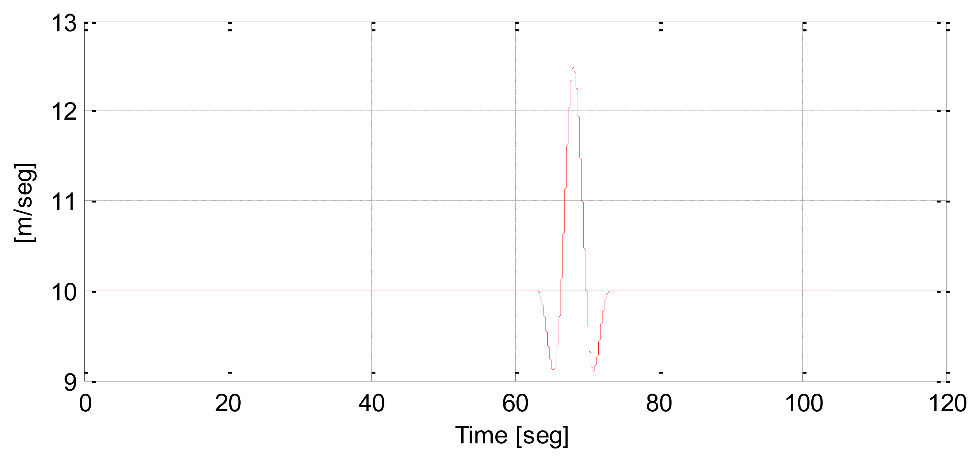
Another wind speed realization utilized in this paper is the Extreme Operating Gust (EOG), as shown in Figure 2. This gust is defined by the IEC 61400 norm. In this case, the wind blows a little less before a high wind speed increment. This wind speed shape allows us to see the pitch control behaviour. When there is a small wind speed fall a power lack results and the control reduces the pitch angle trying to prevent this effect. After this wind speed fall, if there is a high wind speed increment, the turbine captures a lot of energy, forcing the controller to increase dramatically the pitch angle. Consequently, this realization provides a lot of information about control behaviour.
The EOG model parameters are the following:
Wind turbine radius: 11.25 m;
Class: IIIA.
5. Control by Conventional Algorithm
5.1. Wind Turbine Control
A variable speed, variable pitch wind turbine has two main control loops: The torque loop and the pitch loop. The torque loop tries to follow these objectives:
To capture the maximum power at low wind speeds;
To obtain constant power from the wind when the turbine is above the rated rotor speed;
To make a smooth torque transition between these two modes.
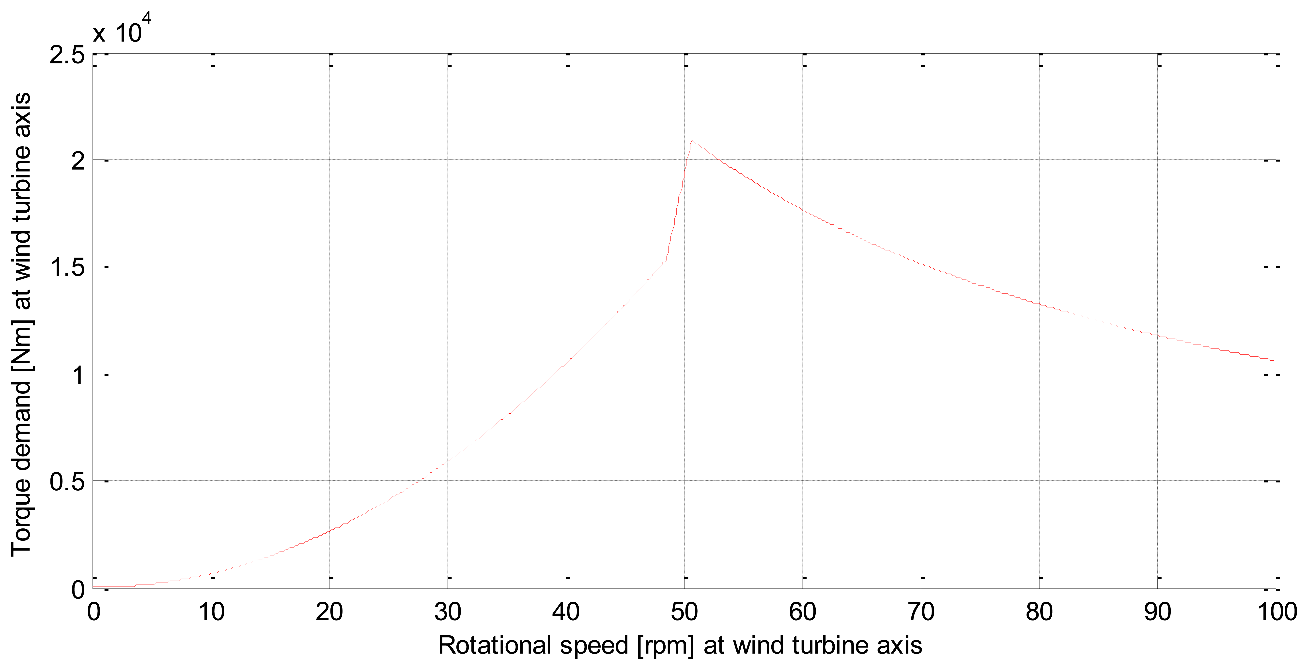
According to these objectives, the relationship between torque setpoint and rotor speed is presented in Figure 3.
When the wind turbine works below the rated speed, the torque demand is calculated as follows:
Cp_max: maximum power coefficient;
η: power train efficiency;
λoptimal: tip speed radio at maximum power coefficient.
When the wind turbine works above the rated speed, the torque demand is calculated as follows:
Pnom: rated wind turbine power.
The transition between these two curves is made linearly. This allows a smooth torque transition between them. The first curve tries to obtain the maximum power from the wind. In this stage the pitch angle is set to zero. The second curve tries to keep the rated power when the wind turbine is above the rated rotor speed. In this stage the pitch angle is variable, and it is calculated by a pitch controller. It is important to notice that the performance has to be taken into account.
The pitch controller has the objective of keeping the wind turbine speed at a certain setpoint. A typical controller structure is a PI with gain scheduling. A good technique can be found in [19]:
β*: pitch angle setpoint;
Kp: proportional gain;
w*: wind turbine angular speed setpoint;
βTi: integration time.
The pitch actuator model is described as follows:
β: pitch angle;
τpa: pitch actuator's position loop time constant.
A τpa time constant has been identified after several trials made with the pitch actuator. In this work, the pitch time rate has been limited to 10°/s. This limit is very common in this kind of applications. In fact, a greater pitch time rate can dramatically increase the structural fatigue. The PI controller parameters can be calculated by the formulae given at [19]. The controller parameters can be defined as follows:
wn: design natural pulsation;
wo: nominal operating wind turbine angular speed;
ε: design damping coefficient;
q1, q2: captured wind turbine power sensibility's linear regression coefficients.
The wind turbine power sensibility can be estimated from the power coefficient surface. Once this sensibility has been estimated the control parameters can be calculated following Equation (10).
5.2. Wind Turbine Speed Setpoint Conventional Algorithm
The conventional rotor speed setpoint algorithm is based on real pitch values. Basically, the rotor speed setpoint is set to its rated value. With higher wind speed, the pitch angle will take higher values. In this situation, when sudden falling wind gusts appear, rotor speed decreases causing loss of electrical power. This loss of production can be avoided when there is a high wind speed, if the rotor speed setpoint is slightly increased. This increment is usually set depending on the pitch angle. A more detailed explanation of this algorithm can be found in [20]. In our study, we have taken this algorithm as conventional example. It is important to remark that these setpoint changes are smoothed by a first order filter with large time constant. The main problem of this algorithm is that it does not take into account the rotor speed acceleration. Thus, a wind speed gust may arrive at high rotor speed while having a high setpoint, resulting in a serious risk as it gets closer from the tower resonance.
6. Reinforcement Learning Based Rotor Speed Setpoint
The first new solution experimented in this work is based on a Reinforcement Learning (RL) based rotor speed setpoint. The main reason for this choice is that the rotor speed setpoint has to be calculated following several opposed criteria and the decision scenario is a stochastic one: the wind speed is a very stochastic process. The two main criteria are:
To capture as much power as possible. To achieve this objective, it is necessary to maintain the rotor speed at high values when the wind speed is above the rated value. So, the rotor speed has to be maintained at high values although a wind speed gust decreases during a short time.
To stay as far as possible from the resonance and reduce the load fatigue. So, the rotor speed has to be reduced to avoid a structural damage.
This kind of problems can be posed as a Markov Decision Process (MDP), and the chosen optimization method is the Q-learning. This technique is applied in stochastic scenarios for multi elements control systems with high success [21]. Also, the RL technique has been applied to wind turbine control in [5]. In this work, the RL has been applied to rotor speed setpoint calculation. The Q matrix has two main input variables: the state and the action. The state has been defined as the Cartesian product between rotor speed and acceleration levels. These variables have been quantified in different levels as explained below.
s: rotor state defined as the Cartesian product;
wstate: rotor speed level;
wrated: rated rotor speed;
αstate: rotor angular acceleration level;
α: rotor angular acceleration;
αrated: rated rotor angular acceleration.
The defined actions are three: High, Medium and Low rotor speed setpoint. When the control system is working with high wind speed and the angular acceleration is negative, high rotor speed setpoint prevents the power from falling. On the other hand, if the rotor speed is high but the acceleration is positive, low rotor speed setpoint prevents the rotor speed from getting closer to resonance speeds. There are different discrete states, and in each state different actions can be chosen. As it may not be clear which is the best action in each state, the reinforcement matrix Q (s, a) must be estimated. In fact, this matrix changes with time, or with the wind turbine placement. This estimation has been built by means of a Q-learning algorithm. Each time the state and its action are calculated the corresponding Q (s, a) matrix element is actualized following the law below:
Qt (s, a): reinforcement matrix at t instant;
a: possible action taken for each s rotor state;
δ: learning ratio;
Rt: instant reward.
The δ the learning ratio must be between zero and one. In our case, this parameter has been set to 0.2. The Rt is the reinforcement obtained at instant t. This variable is evaluated by measuring the captured power and the rotor speed error. Every instant the state is calculated and the reward maximizing action is selected. The rotor speed setpoint is defined by the selected action. There are only three possible actions. The first one imposes high rotor speed setpoint value (2% above the nominal rotor speed). The second one imposes a medium rotor speed setpoint value (the nominal rotor speed). Finally, the third one imposes low rotor speed setpoint (2% below the nominal rotor speed):
Finally the learning algorithm updates the Q (s, a) element.
6.1. Reward Function
The reward function can be expressed as follows:
error: rotor speed error defined between rotor speed and its setpoint;
errorrated: rated rotor speed error.
This function depends on the captured power and on the rotor speed error. The function is the product between two sigmoid terms. The first term gives a low value when the captured power is low, but has a horizontal asymptote that goes to one when the power arrives to infinity. In fact, this term is 0.73 at the rated power. The second term has the same sigmoid function, but in this case the positive rotor speed errors are not penalized because they appear when the wind speed is low. When the rotor speed error is negative, as when there is an over speed, the term decreases because it is closer to the resonance speed. This reinforcement function is always between zero and one. This mathematical property is very desirable because it prevents numerical instabilities in the learning process. The algorithms are compared according to the mean value given by this function along the different wind speed regimes.
7. Pitch Based Rotor Speed Setpoint Using PSO
The second new solution experimented in this work is based on a metaheuristic optimization using the Particle Swarm Optimization (PSO) method. PSO seeks the best parameters for a proposed pitch based rotor speed setpoint function. This proposed function is used to control the wind turbine by pitch angle, which is the only input variable utilized as proposed in the literature [20]. The PSO algorithm-based rotor speed setpoint is explained in this point. First, a mathematical definition of PSO algorithm applied to this work is provided. Secondly, the tuning parameters used are explained and thirdly, the strategy to apply the PSO optimized parameters to evaluation function is exposed.
7.1. Mathematical Definition
PSO is a metaheuristic technique [22] inspired by the collective behaviour exhibited by animals which consists on aggregating together and acting like a single entity capable to move or to stay without a clear guiding leader.
The PSO computational method iteratively optimizes by proposing new solutions based on information of previous results of each particle and the neighbour particle's experiences. The mathematical implementation of PSO method applied to this problem follows. More details can be found in [23].
Mathematically, the search space is defined as A⊂Rn, where n is the number of variables. In our case, there are two dimensions or operation variables: a and α. The first dimension a represents the lower bound from which we start applying the rotor speed setpoint algorithm. The second dimension α represents an exponential parameter that modules the rotor speed setpoint policy sharpness. Each particle is a candidate solution that keeps the values of operation variables, the position in the search space defined in each iteration k:
A particle i moves from one point xi(k) of n dimension to another xi(k+1) with a velocity ui(k) where i can be a particle between 1 and N. Velocity at iteration k to particle i is denoted as:
The best positions that have ever been visited until iteration k by each particle are stored. Each particle only has memory to store the last best position and it is denoted as:
The best position that N particles have visited at iteration k is denoted by g(k):
7.2. Parameters Used
In PSO there are some parameters to be set:
Number of particles (N) it influences in the computational time;
Stop condition: defined by the maximum number of iterations T;
Constraints: Particle positions move between boundaries to fulfil the constraints. Particles must satisfy amin < a < amax and αmin < α < αmax;
Inertia Weight mi is a parameter of particles that exerts resistance to change the motion;
Cognitive parameter (c1) controls the influence of each particle with respect to its best performance found so far;
Social parameter (c2) controls the experience influence of each particle with respect to the best position found by its society.
High values of c1 and c2 provide new points in relatively distant regions of the search space, therefore achieving a better global exploration. On the other hand, the selection of smaller values for these parameters, with c1 > c2 condition, performs refined local search around the best positions achieved previously.
Random values (r1, r2): The r1 and r2 represent uniform distribution random values between 0 and 1. The velocity is updated every iteration. The following equations calculate the particles direction velocity as:
The position is updated from iteration k to k+1 by:
7.3. Assessment Function
The novelty in this paper resides in the function set Equation (15), indexed by a and α parameters, a new pitch based rotor speed setpoint algorithm:
In order to maintain the continuity of the setpoint function, K is defined as follows:
Δwmax is the maximum rotor speed setpoint increment; b is the pitch angle value for which the algorithm applies Δwmax as setpoint increment. These two parameters are set according to our wind turbine dynamics:
The proposed rotor speed setpoint function can express the conventional algorithm when α is equal to one. Two operation parameters need to be optimized. Particles move in a two dimensional space defined by a and α. PSO algorithm optimizes the mean reward of Equation (14). Parameter a is the pitch angle value for which the algorithm does not apply any setpoint increment. Parameter α is an exponent coefficient that increases or decreases the slope of the setpoint function.
8. Results and Comparison
A comparison between the four main rotor speed setpoint policies is carried out:
Constant, which maintains the rotor speed setpoint in a nominal value;
Conventional, which increases the rotor speed setpoint with the pitch angle. This algorithm has been modelled with α = 1, according to Equations (20) and (21);
The proposed RL, which takes into account the rotor speed and the acceleration to change the rotor speed setpoint, according to Equations (11), (12) and (13);
The proposed PSO, which increases the rotor speed setpoint with the pitch angle with an exponential α value, according to Equations (20) and (21).
These algorithms are going to be evaluated in two mains aspects:
Captured power. This value is the mean value of the captured power along certain time span;
Rotor speed error. This value only evaluates the negative error values.
In this comparison the wind speed series utilized are based on EOG models and turbulence wind speed series generated by TurbSim program [18]. The mean wind speeds are 6, 8, 10, 12, 14, 16 and 20 m/s. The turbulence parameters used in these series are given in Section 4.
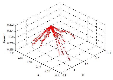
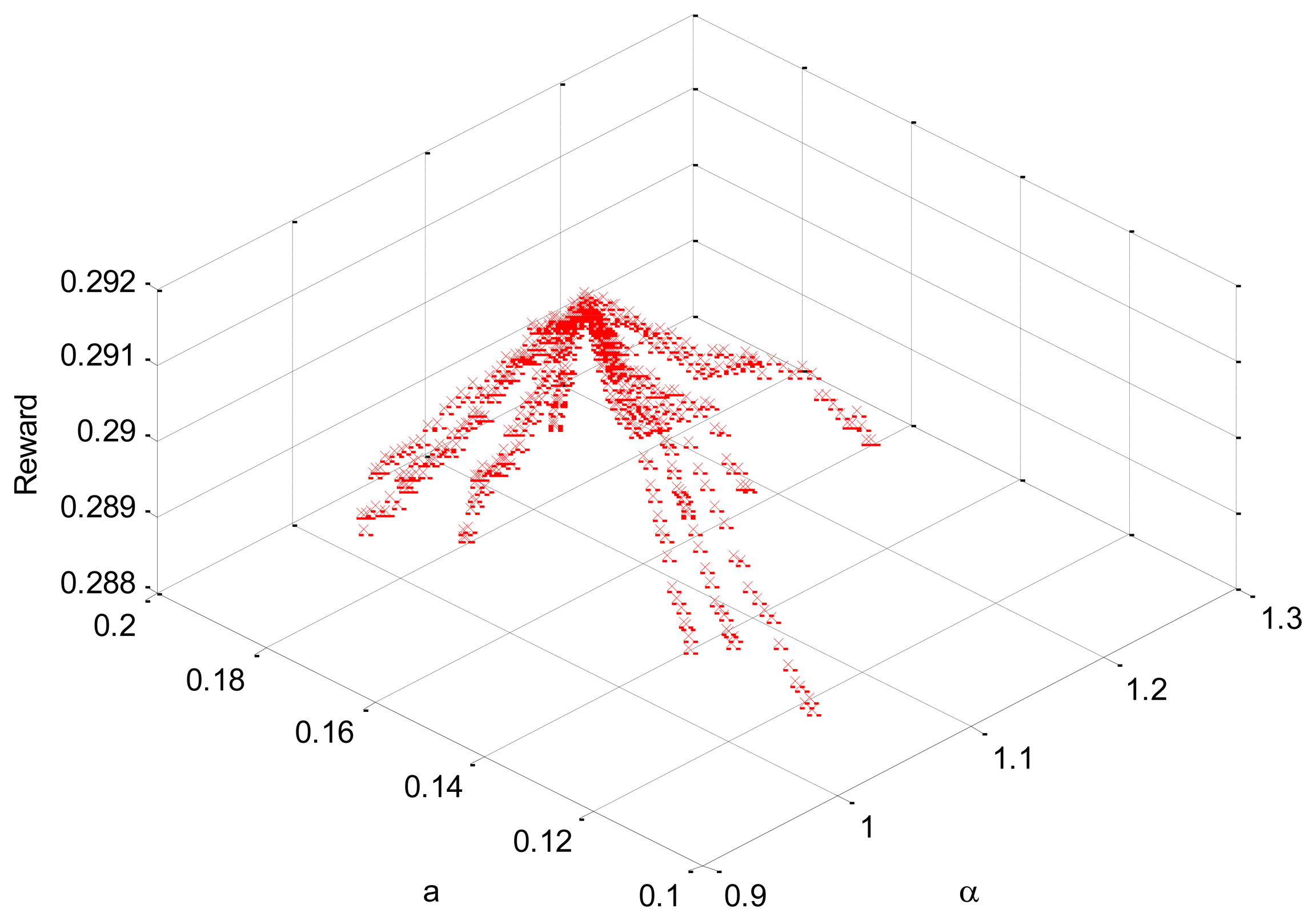
PSO simulations have been carried out with a number of particles in between 40 and 400. Figure 4 shows the results of one of these simulations with 40 particles. All simulations have been executed with c1 = 0.001 and c2 = 0.01; inertia weight = 0.09; number of iterations = 50. Different operation variable spans were tested. Specifically, the spans for Figure 4 were:
0.2·b < a < 0.6·b; 0.9 < α < 1.2 with 40 particles.
Other tested variable spans were:
0.2·b < a < 0.9·b; 0.2 < α < 0.9 with 40 particles;
0.2·b < a < 0.9·b; 0.5 < α < 1.5 with 400 particles;
0.2·b < a < 0.99·b; 0.2 < α < 5 with 400 particles.
All simulations lead us to the same optimal point.
Result values are summarized in Table 1. The PSO algorithm obtains the best mean reward, which improves in 10.67% the constant algorithm and 0.48% the conventional algorithm. The authors estimate that RL algorithm does not have good reward values because of two main reasons:
The algorithm has more input variables (rotor speed and acceleration) than the other ones (pitch angle). This increases the complexity of RL adjustment process.
The RL states have been discretized into a very low number of possibilities in order to reduce the tail of Q (s, a) matrix elements. This choice implies a reduction of improvement capacity.
Mean Reward is evaluated along 800 s time span following the equation below:
9. Conclusions and Future Work
In this paper we have presented intelligent optimization techniques in wind turbine rotor speed setpoint control algorithms. Setpoint algorithms were compared in order to capture as much mean power as possible while avoiding the tower resonance on a 100 kW wind turbine. RL and PSO algorithms were used, together with constant and conventional rotor speed setpoint algorithms for comparison purposes.
Results show that the proposed PSO based rotor speed setpoint algorithm is the best approach in order to improve the proposed reward function. This algorithm is easy to implement in Wind Turbine Control systems and it does not require much computational power. It improves a constant approach, which is very common, in 10.67%. It also improves the more sophisticated conventional approach in 0.48%.
We estimate that RL algorithm has a good potential in this problem but it needs a more complex state definition in order to improve its reward mean value. This implies a heavy increase of computational requirements. Further exploration of these alternatives is envisaged in a near future.
Another important potential improvement is to change the proposed reward function in Equation (14) in order to take into account the turbine blade root load, due to its influence in the structural fatigue. A good starting point for this redefinition is described in [24].


| Metric | Setpoint algorithm | |||
|---|---|---|---|---|
| Constant | Conventional | RL | PSO | |
| Mean reward | 0.2625 | 0.2891 | 0.2500 | 0.2905 |
| Improvement PSO | 10.67% | 0.48% | 16.20% | |
Acknowledgments
This research was supported by the Basque Government through the projects IG-2011/0000794, S-PE11UN061 and S-PE12UN015, and by the Argolabe Ingeniería SL Company. Some of the authors belong to Computational Intelligence Group of the University of the Basque Country (UPV/EHU), supported by the Basque Government.
- Conflicts of Interest: The authors declare no conflict of interest.
References
- Lyu, J.-K.; Heo, J.-H.; Park, J.-K.; Kang, Y.-C. Probabilistic Approach to Optimizing Active and Reactive Power Flow in Wind Farms Considering Wake Effects. Energies 2013, 6, 5717–5737. [Google Scholar]
- Bellman, R. A Markovian Decision Process. J. Math. Mech. 1957, 6, 679–684. [Google Scholar]
- Byon, E.; Ntaimo, L.; Ding, Y. Optimal Maintenance Strategies for Wind Turbine Systems under Stochastic Weather Conditions. IEEE Trans. Reliab. 2010, 59, 393–404. [Google Scholar]
- Byon, E.; Ding, Y. Season-Dependent Condition-Based Maintenance for a Wind Turbine Using a Partially Observed Markov Decision Process. IEEE Trans. Power Syst. 2010, 25, 1823–1834. [Google Scholar]
- Sedighizadeh, M.; Rezazadeh, A. A Modified Adaptive Wavelet PID Control Based on Reinforcement Learning for Wind Energy Conversion System Control. Adv. Electr. Comput. Eng. 2010, 10, 153–159. [Google Scholar]
- Fernandez-Gauna, B.; Manuel Lopez-Guede, J.; Zulueta, E.; Grana, M. Learning Hose Transport Control with Q-Learning. Neural Netw. World 2010, 20, 913–923. [Google Scholar]
- Fernandez-Gauna, B.; Lopez-Guede, J.M.; Grana, M. Concurrent Modular Q-Learning with Local Rewards on Linked Multi-Component Robotic Systems. In Foundations on Natural and Artificial Computation; Ferrández, J.M., Sánchez, J.R.A., de la Paz, F., Toledo, F.J., Eds.; Springer: Berlin/Heidelberg, Germany, 2011; Volume 6686, pp. 148–155. [Google Scholar]
- Lopez-Guede, J.M.; Grana, M.; Zulueta, E. On Distributed Cooperative Control for the Manipulation of a Hose by a Multirobot System. In Hybrid Artificial Intelligence Systems; Corchado, E., Abraham, A., Pedrycz, W., Eds.; Springer: Berlin/Heidelberg, Germany, 2008; Volume 5271, pp. 673–679. [Google Scholar]
- Manuel Lopez-Guede, J.; Fernandez-Gauna, B.; Grana, M.; Zulueta, E. Empirical Study of Q-Learning Based Elemental Hose Transport Control. In Hybrid Artificial Intelligent Systems; Corchado, E., Abraham, A., Pedrycz, W., Eds.; Springer: Berlin/Heidelberg, Germany, 2011; Volume 6679, pp. 455–462. [Google Scholar]
- Cai, X.; Zhu, J.; Pan, P.; Gu, R. Structural Optimization Design of Horizontal-Axis Wind Turbine Blades using a Particle Swarm Optimization Algorithm and Finite Element Method. Energies 2012, 5, 4683–4696. [Google Scholar]
- Garcia-Sanz, M.; Oses, J.A. Evolutionary Algorithms for Automatic Tuning of QFT Controllers. In Modelling, Identification, and Control; Hamza, M.H., Ed.; ACTA Press: Calgary, AB, Canada, 2004. [Google Scholar]
- Burton, T.; Sharpe, D.; Jenkins, N.; Bossanyi, E. Wind Energy Handbook; John Wiley & Sons: Hoboken, NJ, USA, 2001. [Google Scholar]
- Hammerum, K. A Fatigue Approach to Wind Turbine Control. Master's Thesis, Technical University of Denmark, Kongens Lyngby, Denmark, December 2006. [Google Scholar]
- Abad, G.; Lopez, J.; Rodriguez, M.; Marroyo, L.; Iwanski, G. Doubly Fed Induction Machine: Modeling and Control for Wind Energy Generation, 1st ed.; Wiley-IEEE Press: Hoboken, NJ, USA, 2011; pp. 1–640. [Google Scholar]
- Wright, A.D. Modern Control Design for Flexible Wind Turbines; Technical Report NREL/TP-500-35816; National Renewable Energy Laboratory: Golden, CO, USA; July; 2004. [Google Scholar]
- Jonkman, J.M.; Buhl, M.L. FAST User's Guide; Technical Report NREL/EL-500-38230. National Renewable Energy Laboratory: Golden, CO, USA, August 2005. Available online: http://wind.nrel.gov/designcodes/simulators/fast/fast.pdf (accessed on 17 June 2014).
- Hau, E. Wind Turbines—Fundamentals, Technologies, Application, Economics; Springer: Berlin, Germany, 2013. [Google Scholar]
- Kelley, N.; Jonkman, B. NWTC Computer-Aided Engineering Tools (TurbSim). 2012. Available online: http://wind.nrel.gov/designcodes/preprocessors/turbsim/ (accessed on 17 June 2014). [Google Scholar]
- Hansen, M.H.; Hansen, A.; Larsen, T.J.; Øye, S.; Sørensen, P.; Fuglsang, P. Control Design for a Pitch-Regulated, Variable Speed Wind Turbine; Risø-R Report Risø-R-1500(EN); Risø National Laboratory: Roskilde, Denmark; January; 2005. [Google Scholar]
- Van der Hooft, E.L.; Schaak, P.; van Engelen, T.G. Wind Turbine Control Algorithms; DOWEC-F1W1-EH-03-094/0; Dutch Ministry of Economic Affairs: The Hague, The Netherlands; December; 2003. [Google Scholar]
- Fernandez-Gauna, B.; Manuel Lopez-Guede, J.; Grana, M. Towards Concurrent Q-Learning on Linked Multi-Component Robotic Systems. In Hybrid Artificial Intelligent Systems; Springer: Berlin/Heidelberg, Germany, 2011; Volume 6679, pp. 463–470. [Google Scholar]
- Kennedy, J.; Eberhart, R. Particle swarm optimization. Proceedings of the IEEE International Conference on Neural Networks, Perth, Australia, 27 November–1 December 1995; pp. 1942–1948.
- Clerk, M. Particle Swarm Optimization; John Wiley & Sons: Hoboken, NJ, USA, 2010. [Google Scholar]
- Lee, G.; Byon, E.; Ntaimo, L.; Ding, Y. Bayesian Spline Method for Assessing Extreme Loads on Wind Turbines. Ann. App. Stat 2013, 7, 2034–2061. [Google Scholar]
© 2014 by the authors; licensee MDPI, Basel, Switzerland. This article is an open access article distributed under the terms and conditions of the Creative Commons Attribution license ( http://creativecommons.org/licenses/by/3.0/).
Share and Cite
González-González, A.; Etxeberria-Agiriano, I.; Zulueta, E.; Oterino-Echavarri, F.; Lopez-Guede, J.M. Pitch Based Wind Turbine Intelligent Speed Setpoint Adjustment Algorithms. Energies 2014, 7, 3793-3809. https://doi.org/10.3390/en7063793
González-González A, Etxeberria-Agiriano I, Zulueta E, Oterino-Echavarri F, Lopez-Guede JM. Pitch Based Wind Turbine Intelligent Speed Setpoint Adjustment Algorithms. Energies. 2014; 7(6):3793-3809. https://doi.org/10.3390/en7063793
Chicago/Turabian StyleGonzález-González, Asier, Ismael Etxeberria-Agiriano, Ekaitz Zulueta, Fernando Oterino-Echavarri, and Jose Manuel Lopez-Guede. 2014. "Pitch Based Wind Turbine Intelligent Speed Setpoint Adjustment Algorithms" Energies 7, no. 6: 3793-3809. https://doi.org/10.3390/en7063793
APA StyleGonzález-González, A., Etxeberria-Agiriano, I., Zulueta, E., Oterino-Echavarri, F., & Lopez-Guede, J. M. (2014). Pitch Based Wind Turbine Intelligent Speed Setpoint Adjustment Algorithms. Energies, 7(6), 3793-3809. https://doi.org/10.3390/en7063793