1. Introduction
As a result of the development of new paradigms, such as cloud computing, e-commerce and social networks, data center power consumption has increased significantly around the world in recent years (e.g., [
1,
2,
3]). Large data centers are becoming critical elements in the performance of daily tasks [
4]. In fact, data centers now account for around 1.5% of the total power consumed in the U.S. and represent a cost of $4.5 billion, a share that is expected to increase [
5]. Therefore, a great deal of current research is focused on reducing that consumption (e.g., [
6,
7,
8]). On the other hand, optimization techniques applied to saving energy have developed significantly since 2000 [
9].
The conclusions of such studies are highly relevant to information technology (IT) companies when considering ways to minimize operational costs and maximize sustainability [
10].
Nowadays, some works aim at reducing energy consumption of data centers. Gandhi [
11] performs an analysis of the effectiveness of dynamic power management in data centers. This simplest of dynamic power management policies reduces the energy consumption by turning off servers when they are not needed. However, the highly abstract nature of the work, which does not consider the electrical components of the data center, may render the results unrealistic.
An interesting approach is presented in [
12] with an integrated solution that tightly couples IT management and cooling infrastructure management to improve overall efficiency of data center operation. Different from this work, we propose a strategy to optimize the electrical flow of data center power infrastructures.
In [
10], the authors discuss the impact of architectural parameters on data center power consumption. The power consumption of BCube [
13], DCell [
14] and Fat-tree [
15] data center structures is analyzed. The results show that the energy consumption of data centers, because they are designed for a much larger number of servers, is higher than necessary.
As opposed to previous works, what is proposed here is an optimization algorithm that would reduce data center energy consumption by improving the electrical energy flow. Additionally, the dependability, cost and sustainability issues are computed through the Energy Flow Model (EFM) and Reliability Block Diagrams (RBD)/Stochastic Petri Nets (SPN) models supported by the ASTRO environment [
16].
This paper extends our previous work [
6,
17] in which an integrated approach for computing sustainability, dependability and cost issues is proposed. The main goal in this current paper is to improve the electrical energy flow of EFM models and, as a result, improve the metrics obtained through that model. The EFM [
18] allows verifying if the energy flow does not exceed the maximum energy capacity that each component can supply (considering electrical equipment) or extract (assuming cooling equipment).
Algorithms are employed to traverse the EFM in order to compute the energy consumption, sustainability impact and the operational cost of data center architectures [
17]. This work proposes a new algorithm to optimize the energy flow between components by taking into account the electrical efficiency of the devices present in the EFM models. The main goal is to improve the energy flow when there are redundant paths available to support the demanded energy. In concise terms, the proposed algorithm (Power Load Distributed Algorithm—PLDA) aims at increasing the utilization of those paths that have higher electrical efficiency levels.
It should be stressed that the EFM has the support of the ASTRO/Mercury environment [
16]. ASTRO is a tool that analyzes power, cooling and IT data center infrastructures. The environment kernel, Mercury, is responsible for performing the evaluation of the supported models (Stochastic Petri nets—SPN; Reliability Block Diagrams—RBD; EFM; and Markov Chain—MC) [
19]. ASTRO provides views for modeling data center power, cooling and IT infrastructures from which non-specialized users may conduct the dependability, sustainability and cost evaluation without the need to be familiar with those formalisms used by Mercury [
16]. Models created through the ASTRO environment are automatically converted to models supported by Mercury (for the dependability evaluation).
A case study is conducted to compare the dependability, sustainability and cost results obtained before and after applying the optimization technique (PLDA algorithm) to different data center power architectures. The computed dependability evaluation employs a hierarchical approach that recognizes the advantages of both stochastic Petri nets (SPN) [
20] and Reliability Block Diagrams (RBD) [
21].
The paper is organized as follows:
Section 2 introduces basic concepts regarding data center infrastructures, sustainability, directed acyclic graphs (DAGs) and dependability;
Section 3 presents an overview of Reliability Block Diagram (RBD);
Section 4 presents an overview of the ASTRO/Mercury environment;
Section 5 describes the Energy Flow Model (EFM);
Section 6 explains the PLDA;
Section 7 applies the adopted methodology;
Section 8 presents a real-world case study; and finally,
Section 9 concludes the paper and suggests directions for future work.
2. Preliminaries
This section discusses the basic concepts needed for a better understanding of the paper and presents an overview of data center infrastructures, followed by an explanation of the concepts of exergy and directed acyclic graphs. Finally, the concepts about dependability are introduced.
2.1. Data Center
With the aim of ensuring availability, a data center is the concentration in one location of the processing and data storage devices responsible for running the business of organizations. Power outages and electrical energy oscillations are important events that a data center must be able to deal with in order to avoid damage to its equipment and provide the high availability demanded. A data center essentially consists of three sub-systems:
The IT infrastructure comprises three main components: servers, network equipment and storage devices. Software services are usually organized in a multi-tier architecture with separate layers for web-servers, application servers and databases.
The cooling infrastructure is responsible for extracting heat from the data center room. It accounts for between 10% and 20% of the total data center energy consumption [
22].
The power infrastructure provides uninterrupted and conditioned electrical energy at the correct voltage and frequency to the IT and cooling sub-systems. The electricity passes through transformers, transfer switches, uninterruptible power supplies (UPS), distribution boards and, finally, to rack power strips [
23]. The current work focuses on the power infrastructure.
2.2. Exergy
There are several interconnected methods of comparing equipment from the point of view of sustainability, for example: respective electrical energy consumption; the materials used in manufacture; or the environmental impact and irreversible environmental losses for future generations. These alternative techniques for measuring sustainability occasionally produce conflicting results. For instance, any particular item of equipment may be considered a better option than another, if despite having higher power consumption, it has a positive impact on the future environment.
Exergy is a metric that estimates the energy consumption efficiency of a system, such as the architecture of a data center. As an index for the global assessment of sustainability, the thermodynamic property of exergy is of great importance. It is defined as the maximal fraction of latent energy that can be theoretically converted into useful work [
24]. A useful illustration would be to compare the exergy of 1 kJ of gasoline with that of 1 kJ of water at ambient temperature. The exergy of the gasoline is much greater, since it can be used to move a truck, but the water at ambient temperature cannot.
2.3. Directed Acyclic Graph
A graph can be described as a structure constituted by two elements: the arcs and vertices. In recent decades, a relationship between algorithms and graphs has been studied. In general, the area of algorithms and graphs may be characterized as one whose primary interest is to solve problems in graphs using algorithms, keeping in mind a computing concern. In this study, the case is repeated once we have a problem in a graph. There are several types of graphs with several special issues (e.g., complete, symmetric, cyclic, directed,
etc.) [
25]. This paper adopts directed acyclic graphs.
A directed graph, D (V,E), is a finite nonempty set, V (vertices), and a set of arcs, E (edges) ordered pairs of distinct vertices [
26]. Thus, in a directed graph, each arc (v,w) has only one direction from v to w. In an acyclic graph, the initial and final vertices cannot be the same for any subpath in the graph.
In this paper, the EFM is a directed acyclic graph. For more details about the graphs, the reader is redirected to [
25,
26].
2.4. Dependability
The dependability of a system can be understood as the ability to deliver a set of services that can be justifiably trusted [
21,
27,
28]. In point of fact, dependability is closely related to the concepts of fault tolerance and reliability.
Reliability is the probability that the system will deliver a set of services for a given period of time. Fault tolerance is the ability of a system not to fail even when there are faulty components [
29]. In fault-tolerant systems, the reliability provides the probability that a system will function even when there are faulty components.
Availability is another important concept that quantifies the mixed effect of both the failure and repair process in a system [
21]. To calculate the availability value of a given device or system, the uptime and the downtime, or the time to failure (TTF) and time to repair (TTR), need to be known. Since the specific uptime and downtime are not accessible, the solution is to use mean values. In such a situation, the commonly adopted metrics are mean time to failure (MTTF) and mean time to repair (MTTR). For more details, the reader should refer to [
21], which also supplies the equations for estimating dependability metrics.
3. Dependability Model—Reliability Block Diagram
The Reliability Block Diagram (RBD) is a combinatorial model that was initially proposed as a technique for calculating the reliability of systems by employing intuitive block diagrams. The technique was then extended to compute availability and maintainability [
21].
The RBD structure establishes a logical interaction between the components, defining which combinations of failed and active elements are able to sustain system operation. Thus, the system is represented by subsystems or components connected according to their function or reliability relationship [
30].
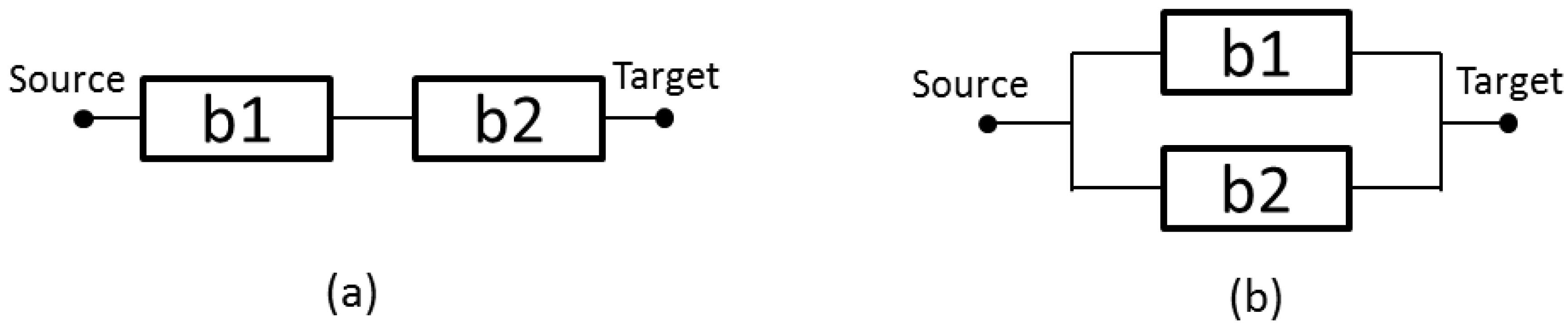
Figure 1a is an illustration of a series arrangement, where the failure of a single component will cause the whole system to cease to function [
31].
Assuming a system with
n independent components, the reliability (instantaneous availability or steady state availability) is calculated by:
where
is the reliability—
(instantaneous availability (
) or steady state availability (
))—of block
.
Figure 1b depicts a parallel arrangement, where the whole system will continue to function, even if only a single component is operational [
31].
Assuming a system with
n independent components, the reliability (instantaneous availability or steady state availability) is calculated by:
Figure 1.
(a) Serial arrangement; and (b) parallel configuration.
Figure 1.
(a) Serial arrangement; and (b) parallel configuration.
A
k-out-of-
n system functions if and only if
k or more of its
n components are functioning. Let
be the success probability of each of those blocks. The system success probability (reliability or availability) is calculated by:
For other examples and closed-form equations, the reader should refer to [
21].
3.1. Structure Function
Structural functions are used to represent the relationship between the individual components and system state. Consider a system,
S, composed by a set of components,
C =
∣ 1 ≤
i ≤
n, where the state of the system,
S, and its components could be either operational or failed and
n is the number of components of the system. Let the discrete random variable,
, indicate the state of component
i; thus:
Additionally, a vector,
x = (
,
, ...,
), represents the state of each component of the system. The state of the system is determined by the states of the components. The structure function,
, maps the system state vector,
x, to one or zero, as shown below:
The blocks (e.g., components) are usually arranged using the following composition mechanisms: series, parallel, k-out-of-n blocks, bridge or even a combination of previous approaches. The following lines highlight the structural and parallel composition utilized in this paper.
: Let
n components,
,
, ...,
, in series; the structural function of these components is represented by:
: Let
n components,
,
, ...,
, in parallel; the structural function of these components is represented by:
3.2. Logic Function
Logical functions have the same goal of structural functions: to indicate a relationship between the states of the components and the state of the system. However, in some cases, simplifying the structure function may not be an easy task [
21]. A logic function of a coherent system may be adopted to simplify the system’s functions through Boolean algebra.
: Let
x = (
,
, ...,
), the vector that represents the state of
n components of a system. The serial logic function (
S) is defined by:
: Let
x = (
,
, ...,
), the vector that represents the state of
n components of a system. The parallel logic function (
S) is defined by:
For more details about structured or logic functions, the reader is redirected to [
21,
32].
4. ASTRO/Mercury Environment
ASTRO is a tool that analyzes power, cooling and IT data center and cloud infrastructures [
16]. The environment’s kernel, named Mercury, is responsible for evaluating the supported models: Stochastic Petri Nets (SPN), Reliability Block Diagrams (RBD), EFM and Markov Chain (MC). Mercury supports the difficulties encountered with RBD modeling (e.g., dependency relationship), which may be solved by SPN or MC.
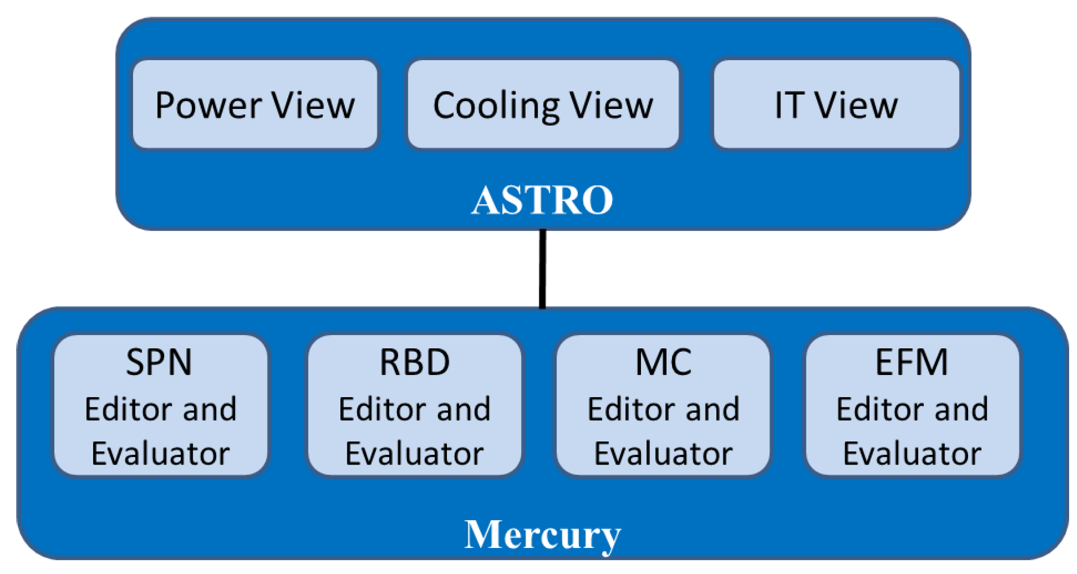
Figure 2 presents the relation between ASTRO and Mercury. It is important to state that the model built through the IT, power and cooling views available in ASTRO can be automatically converted to the models supported by Mercury (for dependability evaluation).
Therefore, in the ASTRO environment, non-specialized users may conduct the dependability, sustainability and cost evaluations without the need to be familiar with those models. This work focuses on the Mercury environment.
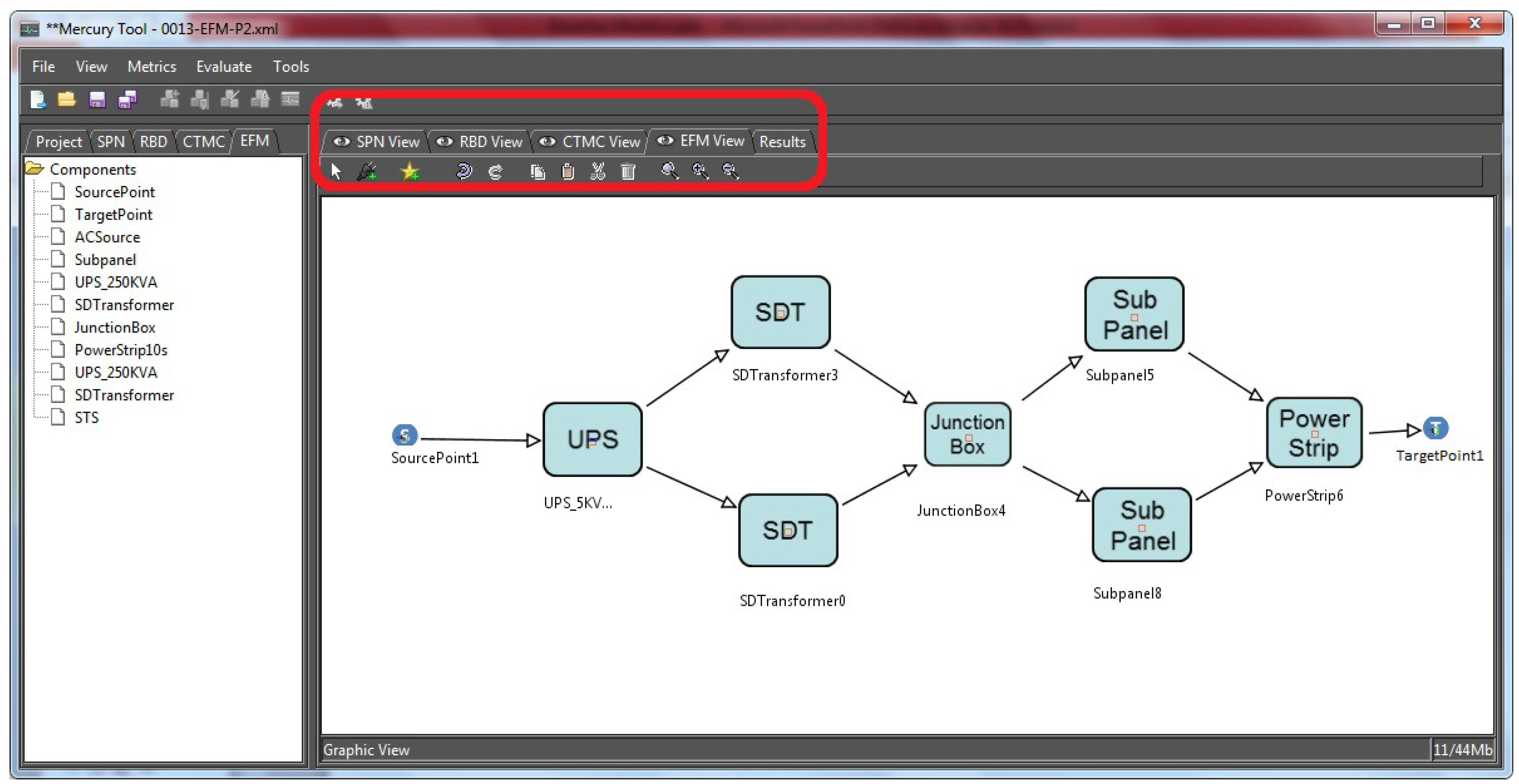
Figure 3 depicts the Mercury environment. The highlighted rectangle shows the set of models available in the Mercury tool. In this figure, an example of the EFM is also depicted.
In the ASTRO/Mercury environment, non-specialized users may conduct the dependability, sustainability and cost evaluations without the need to be familiar with those models.
For more details about the ASTRO/Mercury tool, the reader is redirected to [
16].
Figure 2.
Environment functionalities.
Figure 2.
Environment functionalities.
Figure 3.
Mercury environment.
Figure 3.
Mercury environment.
5. Energy Flow Model
The Energy Flow Model (EFM) [
18] quantifies the energy flow between system components, whilst respecting the maximum energy that each component can provide or extract. The EFM is represented by a directed acyclic graph in which components are modeled as vertices and the respective connections correspond to edges. The following defines the EFM:
, where:
represents the set of nodes (i.e., the components), in which is the set of source nodes, is the set of target nodes and denotes the set of internal nodes, ;
= {(a,b) ∣ a ≠ b} denotes the set of edges (i.e., the component connections).
is a function that assigns weights to the edges (the value assigned to the edge (j, k) is adopted for distributing the energy assigned to the node, j, to the node, k, according to the ratio, w(j,k)/w(j, i), where is the set of output nodes of j);
is a function that assigns to each node the heat to be extracted (considering cooling models) or the energy to be supplied (regarding power models);
is a function that assigns each node with the respective maximum energy capacity;
is a function that assigns each node (a node represents a component) with its retail price;
is a function that assigns each node with the energetic efficiency.
For more details about EFM modeling, the reader is directed to [
18].
Example
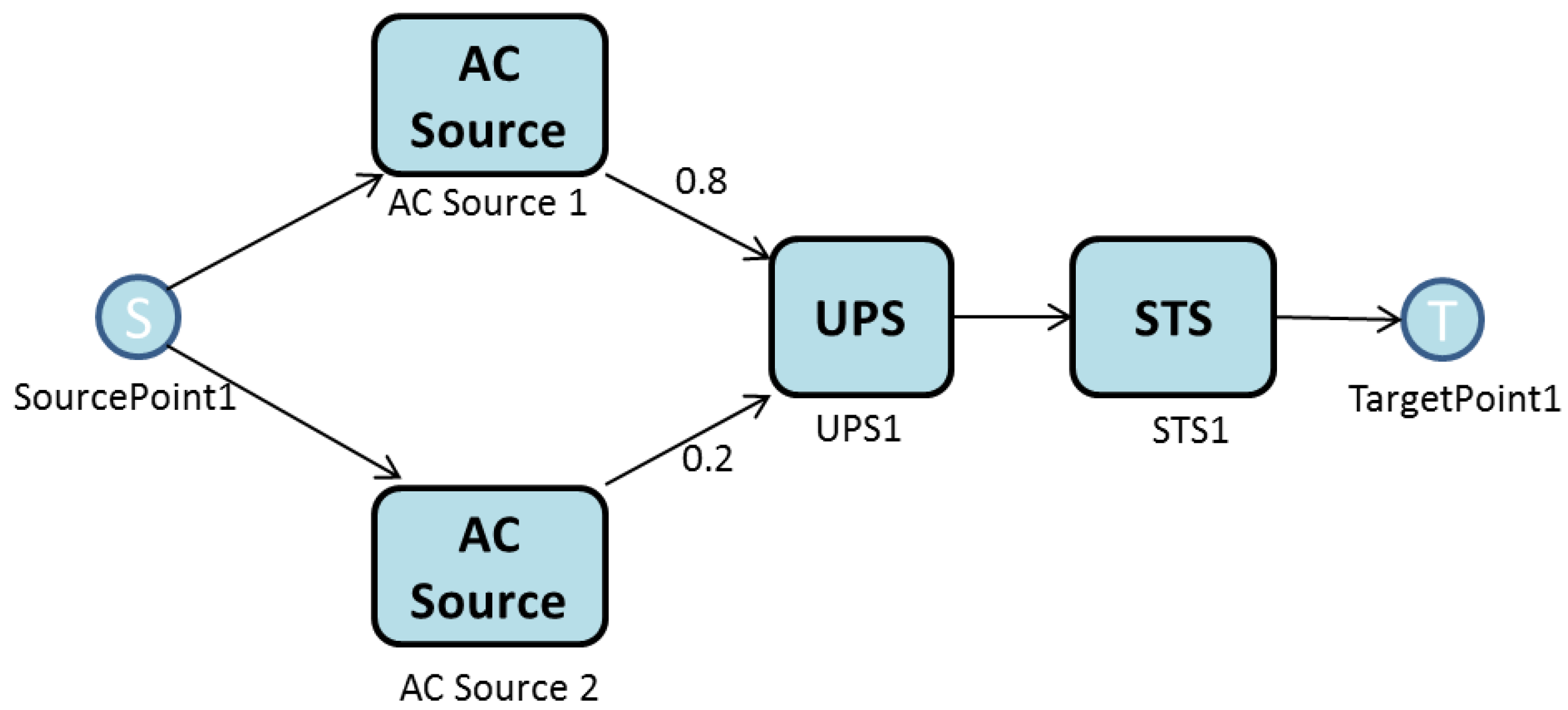
Figure 4 is an example of an EFM. The rounded rectangles equate to the type of equipment, and the labels name each item. The edges have weights that are used to direct the energy flow between the components. For the sake of simplicity, the graphical representation of EFM models hides the default weight, one.
In the present paper, the EFM is employed to compute the overall energy required to provide the necessary energy at the target point. The demanded power associated to TargetPoint1 is 128.25 kW. Thus, since the efficiency of STS1 (Static Transfer Switch) is 95%, the electrical power the STS component must receive is 135 kW.
A similar strategy is adopted for component, UPS1. Since its energy efficiency is 90%, the electrical power flowing through it is 150 kW. From UPS1, the flow is divided between the two AC sources according to the associated edge weights. Therefore, 120 kW of the flow is assigned to ACSource1 and 30 kW to the other. The process continues until SourcePoint1 is reached, which accumulates the total flow.
However, here, the respective weights and efficiency of the ACSource components do not correspond. A weight of 0.8 units is ascribed to the edge that connects the UPS node to ACSource1 and a weight of 0.2 to the other edge that connects the node to ACSource2. This means that ACSource1 supplies four times more power than ACSource2.
It is important to stress that the edge weights are defined by the model designer. There is no guarantee that the designers allocate the best values for that distribution, and the outcome may be higher power consumption. The present paper aims to optimize the edge weight distribution of the EFM model through a Power Load Distribution Algorithm, as explained in
Section 6.
Figure 4.
A simple example of energy modeling with the Energy Flow Model (EFM).
Figure 4.
A simple example of energy modeling with the Energy Flow Model (EFM).
5.1. Cost
The evaluated capacity of cost in a data center is essential for an analysis of return on investment and other business decision processes. This work considers acquisition and operational costs. The acquisition cost is the financial resource required to purchase the data center infrastructure. The operational cost corresponds to the cost of the operation of the data center for a period of time, considering energy consumed, energy cost, period of evaluation and the availability of the data center.
In this paper, the operational cost is utilized as a metric to financial evaluation of the data center, once this metric relates availability and energy consumption. It is computed by the following Equation (
8). In addition, it is important to stress that other costs (e.g., maintenance cost) can be added to this equation.
where: OpCost is the operational cost;
is the electrical energy consumed;
is the energy cost;
T is the assumed period;
A is the availability; and
α is the factor adopted to represent the amount of energy that continues to be consumed when a component has failed.
5.2. Operational Exergy
In this work, the operational exergy is used to measure the environmental impact of the electrical energy waste of the electrical components of the data center. Each electrical component dissipates a fraction of heat, which is not theoretically converted into useful work, called operational exergy.
The lower the value of operational exergy, the lower the environmental impact from the data center infrastructure. Equation (
9) is used to compute the value of operational exergy:
where
is the operational exergy of each device;
T is the period of analysis;
A is the system availability; and
α is the factor that represents the amount of energy that continues to be consumed after a component has failed.
Each type of device uses a specific equation to calculate the operational exergy. The equation used to evaluate a diesel generator is different from that used to evaluate a cooling tower. This study considered only electrical devices, and Equation (
10) is utilized to compute the exergy of each device.
where:
is the total input power of the electrical device; and
η is the delivery efficiency.
For more information, the reader is redirected to [
17].
6. Power Load Distribution Algorithm
A Power Load Distribution Algorithm (PLDA) is proposed to minimize the electrical energy consumption of the EFM models [
18]. The PLDA is based on the Ford-Fulkerson algorithm, which computes the maximum possible flow in a flow network [
33]. The network is represented by a graph, where the transport capacity of the devices is defined in the edges. The algorithm begins by traversing the graph, searching for the best flows between two specific points in the graph. If a particular path lacks the capacity to support all of the flow demanded, then the residual flow is redirected to other paths. The Priority First Search (PFS) is the adopted method for selecting the path between the nodes. The PFS chooses the path according to the highest electrical capacities of nodes in the graph [
34]. For more details about the Ford-Fulkerson algorithm, the reader is referred to [
33].
The flow to be distributed (called demanded electrical energy) is an element of the EFM model. The demand is inserted into the destination vertex and will be the stop criterion of the algorithm. Whilst there is demanded energy in the destination vertex, a “path” is sought to transmit that flow. The choice is made from among the vertices belonging to that path and is the vertex with the lowest capacity.
After each iteration, the value of the aforementioned lowest capacity vertex is subtracted from the demanded value. For every vertex of that path, the flow is increased and the capacity decremented by the value of the transmitted flow. All changes are applied to the EFM model.
The PLDA algorithm is composed of two functions, initialize and PLDA. Algorithm 1 (function Initialize) is responsible for initializing variables, as well as performing calls to the PLDA. The number of calls corresponds to the number of target nodes on the EFM model, G, set as a parameter in Algorithm 1. The first step of the algorithm is to make a copy of the original graph, G. The copy is stored in the variable, R (Line 1). A vector, named ccu, is employed to associate to each node a value that expresses the current capacity utilized by each node. Line 3 initializes the ccu of each node to zero. Next, a repetition structure (Lines 5 to 7) is adopted to perform calls to the PLDA kernel. Finally, the weights on the edges of the EFM model are updated according to the current accumulated vector, ccu (Line 8).
The function PLDA (Algorithm 2) is the kernel of the power load distribution algorithm. Algorithm 2 begins by checking if there is a valid path from the node, n, to the node, s. The n is an element of the set of target nodes, , and the s is an element of the set of source nodes, , of the EFM. A valid path is a path from one node to another where the electrical capacity of all components in this path are respected. The variable, P, is a vector that holds the elements of a valid path (line 2). Once a valid path is verified, a symbol representing infinity is assigned to the variable, pf (line 3). In Line 5, pf receives the value returned by the call to the function, getMinimumCapacity(). This function is responsible for computing the minimum capacity of the paths available. Next, the ccu of each node is updated (Line 8). In addition, the demanded electrical power of the node, n, is also updated (Line 10). The previous steps are repeated until all valid paths have been analyzed. Finally, the residual graph, R, is returned. It is important to stress that only the edge weights are changed from the original graph, G.
| Algorithm 1 Initialize Power Load Distribution Algorithm (PLDA; G) |
- 1:
R = G; - 2:
for N do - 3:
- 4:
end for - 5:
for do - 6:
- 7:
end for - 8:
- 9:
|
| Algorithm 2 PLDA (R, (n), n) |
- 1:
while (isPathValid(R,n,s)) & ( > 0) do - 2:
- 3:
- 4:
for do - 5:
- 6:
end for - 7:
for do - 8:
- 9:
end for - 10:
= - - 11:
end while - 12:
R
|
Example
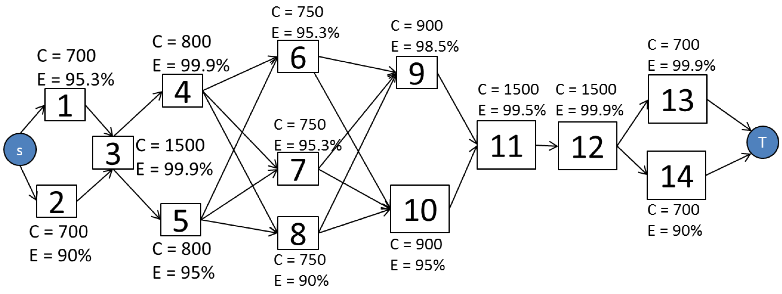
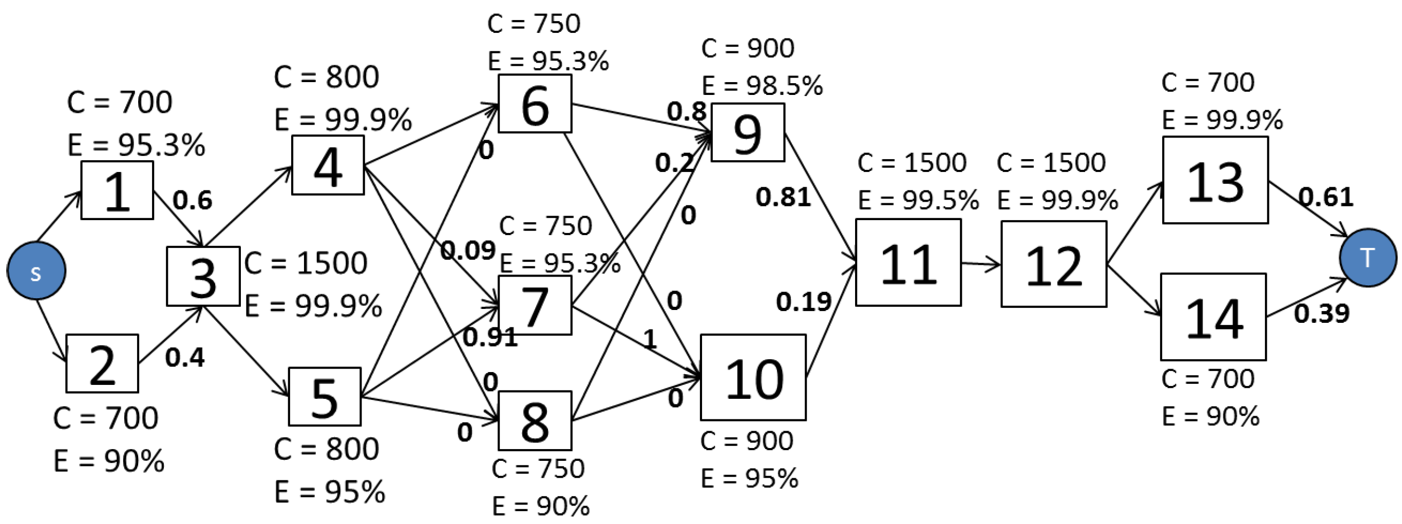
Figure 5 illustrates the EFM model of a specified architecture. In the example, all the edge weights are set to the default value, one. The power flow is computed by traversing the graph from the target to the source node.
Figure 6 depicts the EFM model after the execution of the PLDA. It should be noted that the weights on the edges have changed, optimizing the power flow through a best weights distribution.
Table 1 presents a summary of the results obtained by the PLDA. Column “
Improvement" depicts the improvement. The system efficiency is improved by over 4.2%; consequently, the associated cost and sustainability figures are improved by 4.2% and 20.4%, respectively. Availability results were also computed with RBD/SPN models, but are not included here.
Figure 6.
EFM model after PLDA execution.
Figure 6.
EFM model after PLDA execution.
Table 1.
Summary results before and after PLDA execution.
Table 1.
Summary results before and after PLDA execution.
| Metric | Before | After | Improvement (%) |
|---|
| Availability (%) | 0.99999226 | 0.99999226 | 0 |
| Number of 9 s | 5.111 | 5.111 | 0 |
| Downtime (hs) | 0.0677 | 0.0677 | 0 |
| Input Power (kW) | 1,312.63 | 1,259.64 | 4.2 |
| System Efficiency (%) | 76.18 | 79.38 | 4.2 |
| Operational Cost (USD) | 1,264,849 | 1,213,784 | 4.2 |
| Operational Exergy (GJ) | 9,859.32 | 8,188.11 | 20.4 |
7. Methodology
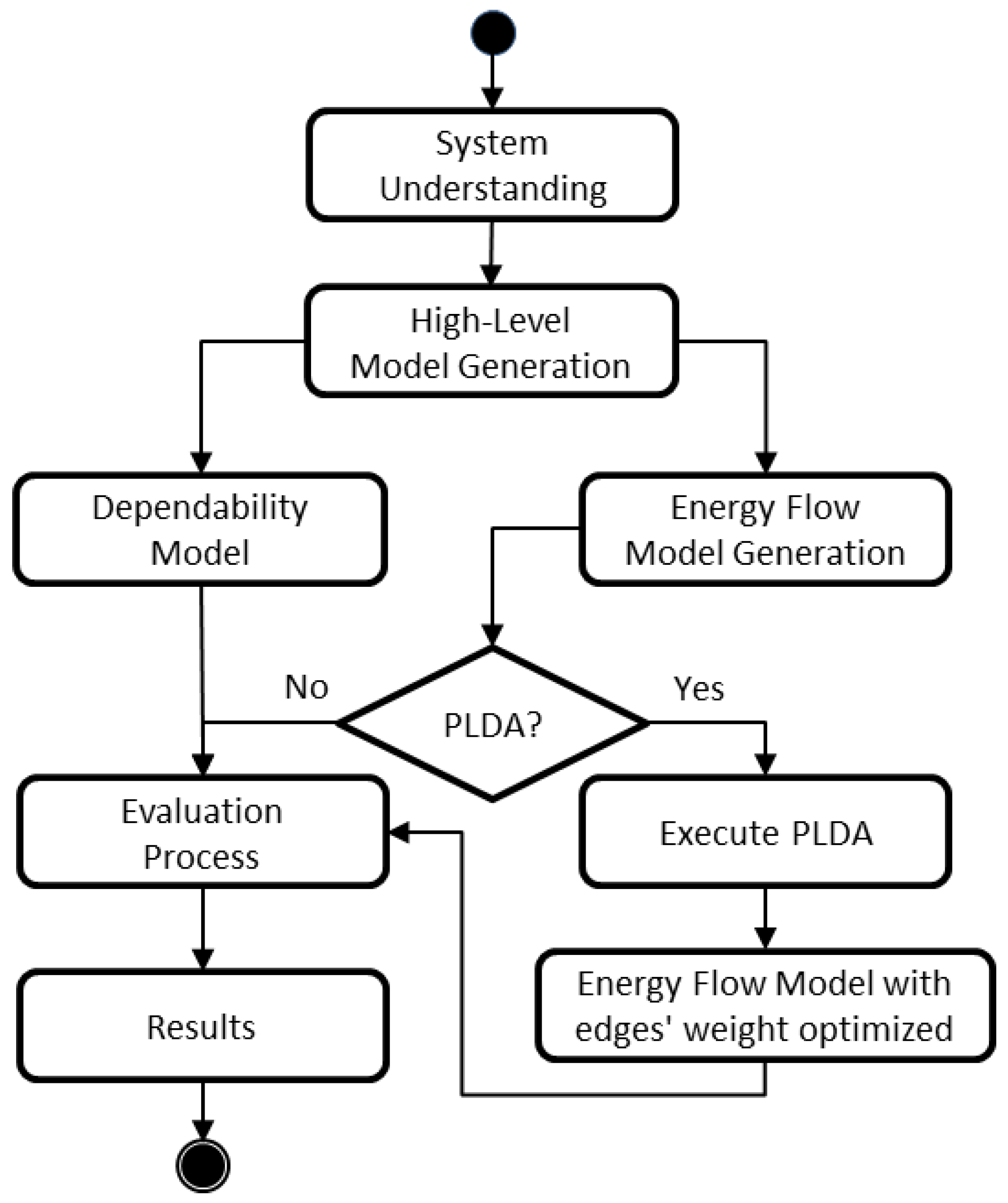
Figure 7 depicts an overview of the allocation methodology. Its first step comprises understanding the system components, interfaces and interactions. This phase should also produce the set of metrics (e.g., input power, availability, reliability, costs) to be evaluated. The next stage is to create the high-level models that represent the data center architecture. These high-level models can be created by adopting the data center views present in the ASTRO tool. The dependability models can be automatically obtained by the models created in ASTRO. Besides, the EFM is also generated.
The PLDA optimizes the energy flow distribution of the EFM models, which are available in the Mercury tool. Therefore, following the adopted methodology, at this time, there are two ways to proceed, the application or not of the PLDA algorithm. If it is executed, then, the algorithm updates the EFM model with different weights on the edges. This optimizes the electrical energy flow distribution of EFM. The next stage is to conduct the evaluation of the dependability model, which is followed by the evaluation of the EFM and takes into account the availability result obtained through the dependability evaluation. Finally, the evaluation results are obtained.
In order to show the applicability of the PLDA algorithm, the results obtained considering the execution of PLDA may be compared with the results from the models that were not optimized. Such comparison is further performed in
Section 8.
8. Case Study
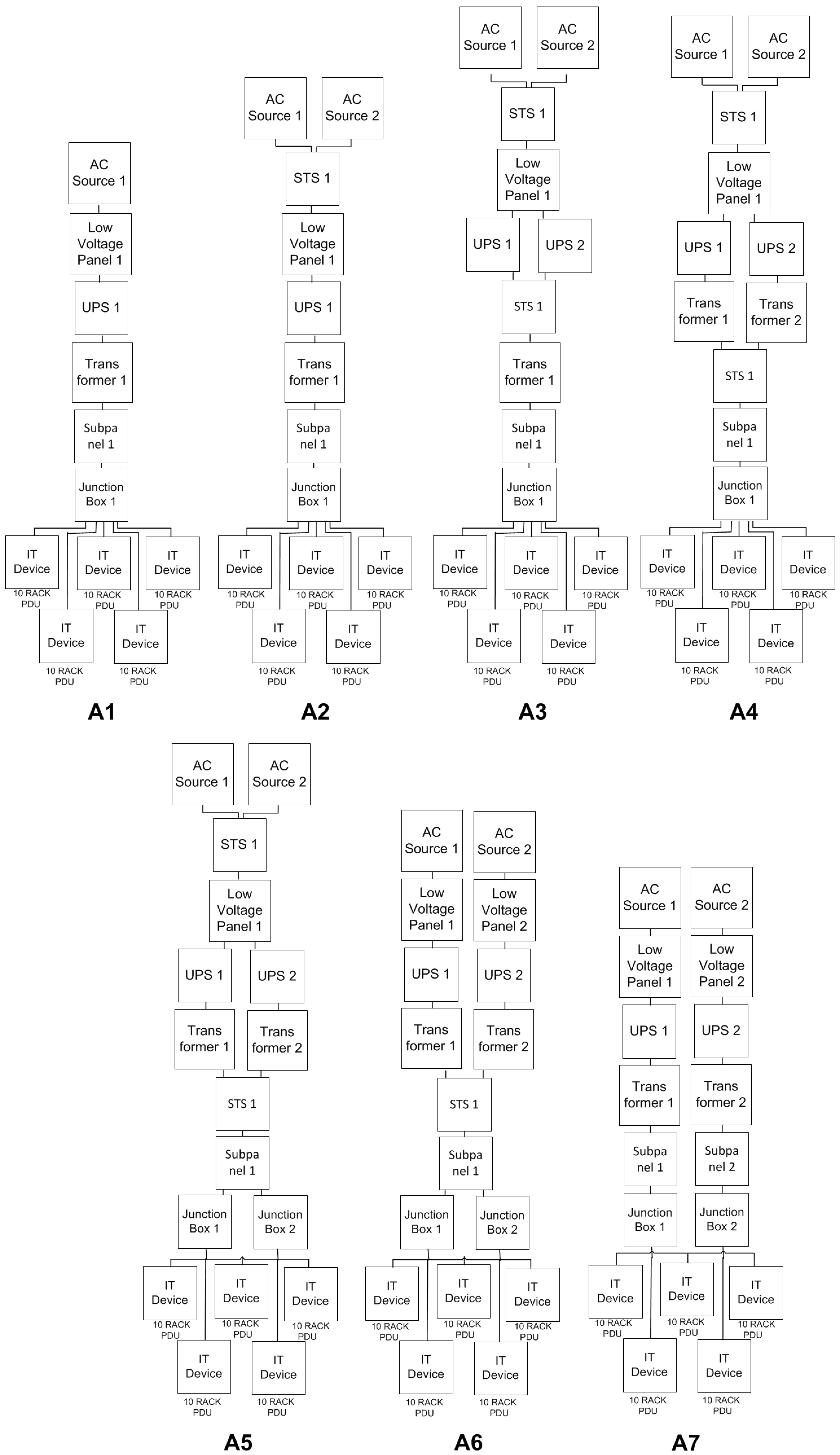
The objective of the case study was to verify the applicability of the PLDA. Seven data center power infrastructures were evaluated (see
Figure 8). For each architecture, the following metrics were calculated: (i) operational exergy; (ii) operational cost; (iii) availability; (iv) number of nines (availability in another view); (v) downtime (year); (vi) input power; and (vii) system efficiency.
Figure 8.
Architectures A1 to A7.
Figure 8.
Architectures A1 to A7.
These values were computed over the period of one year. Each metric was computed before and after the PLDA execution.
8.1. Architectures
The architectures analyzed are similar to those present in HP Labls, Palo Alto, CA, USA [
35]. Beginning from the real power infrastructure depicted in
Figure 8 (A1), the other architectures were defined according to the reliability importance index [
23]. This index identifies the component to be replicated. For instance, in architecture A1, component, ACSource, was indicated to be replicated. Therefore, A2 corresponds to A1 considering component, ACSource, replicated. A similar approach was adopted to propose the other architectures. Typically, the electrical flow in a data center starts from a power supply (
i.e., AC source) and, then, passes through voltage panels, uninterruptible power supply units (UPSs), power distribution units (PDUs) (composed of a transformer and an electrical subpanel), junction boxes and, finally, to rack PDUs (rack power distribution units). As detailed in
Table 2, the case study employs redundant devices with dissimilar electrical efficiencies. The table also lists the maximum energy capacity of each device.
Table 2.
Capacity and efficiency.
Table 2.
Capacity and efficiency.
| Equipment | Efficiency (%) | Capacity (kW) |
|---|
| AC Source 1 | 95.3 | 10,000 |
| AC Source 2 | 90 | 10,000 |
| STS 1 | 99.5 | 1,500 |
| STS 2 | 98 | 1,500 |
| STS 3 | 99.5 | 1,500 |
| SDT (or Transformer) 1 | 98.5 | 5,000 |
| SDT (or Transformer) 2 | 95 | 5,000 |
| Sub Panel 1 | 99.9 | 1,500 |
| Sub Panel 2 | 95 | 1,500 |
| Sub Panel 3 | 99.9 | 1,500 |
| Low Voltage Panel 1 | 99.9 | 1,500 |
| Low Voltage Panel 2 | 95 | 1,500 |
| UPS 1 | 95.3 | 5,000 |
| UPS 2 | 90 | 5,000 |
| Junction Box 1 | 99.9 | 1,500 |
| Junction Box 2 | 98 | 1,500 |
| Power Strip | 95.1 | 5,000 |
8.2. Models
This section presents the models for A5. However, a similar process was followed to evaluate the other architectures (A1–A4, A6 and A7).
Figure 9 illustrates the RBD model for architecture A5.
Figure 9.
Reliability Block Diagram (RBD) model of architecture A5.
Figure 9.
Reliability Block Diagram (RBD) model of architecture A5.
The evaluation of the RBD model provides the availability metric. This is achieved by following these functions.
Table 3 depicts the variables used in Functions (
11)–(
13), their respective equipment and definitions. For more details about the notation of variables and procedures, the reader is referred to [
32]. The MTTF and MTTR values needed to compute the availability were obtained from [
36].
Table 3.
Equipment, associated variables and definitions.
Table 3.
Equipment, associated variables and definitions.
| Equipment | Variables | Definition |
|---|
| AC Source 1 and 2 | AC S1 and AC S2 | AC Source |
| STS 1 and 3 | STS1 and STS3 | Static Transfer Switch |
| Sub Panel 1 | SP1 | Sub Panel |
| Low Voltage Panel 1 | LVP1 | Low Voltage Panel |
| UPS 1 and 2 | UPS1 and UPS2 | Uninterruptible Power Supply |
| Junction Box 1 and 2 | JB1 and JB2 | Junction Box |
| Power Strip | RPDU(1..5) | Power Strip |
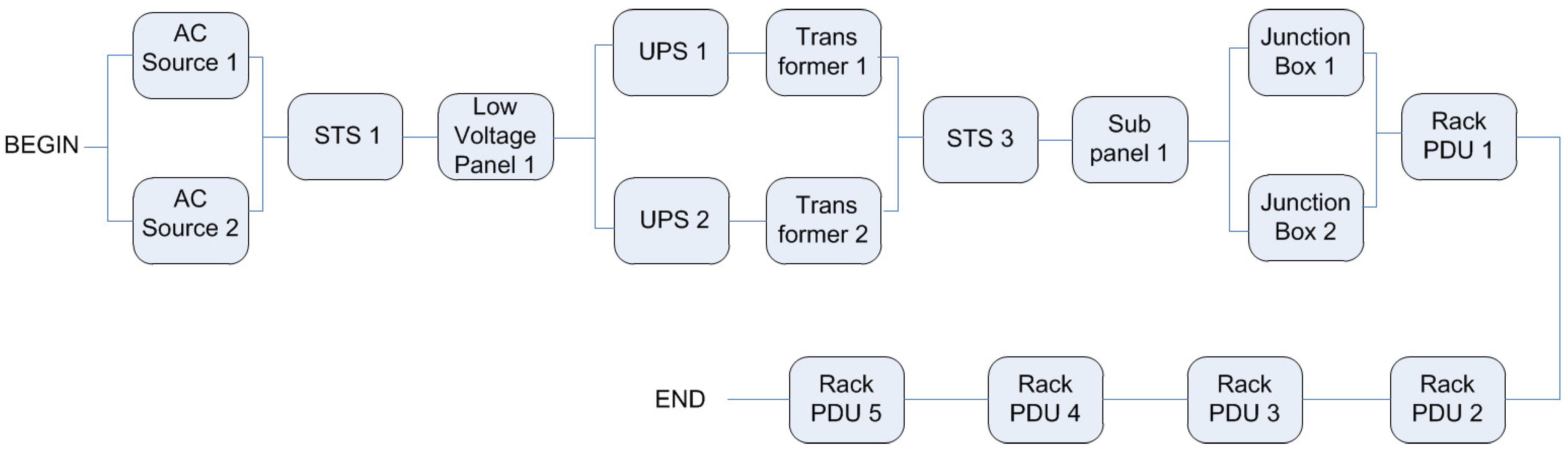
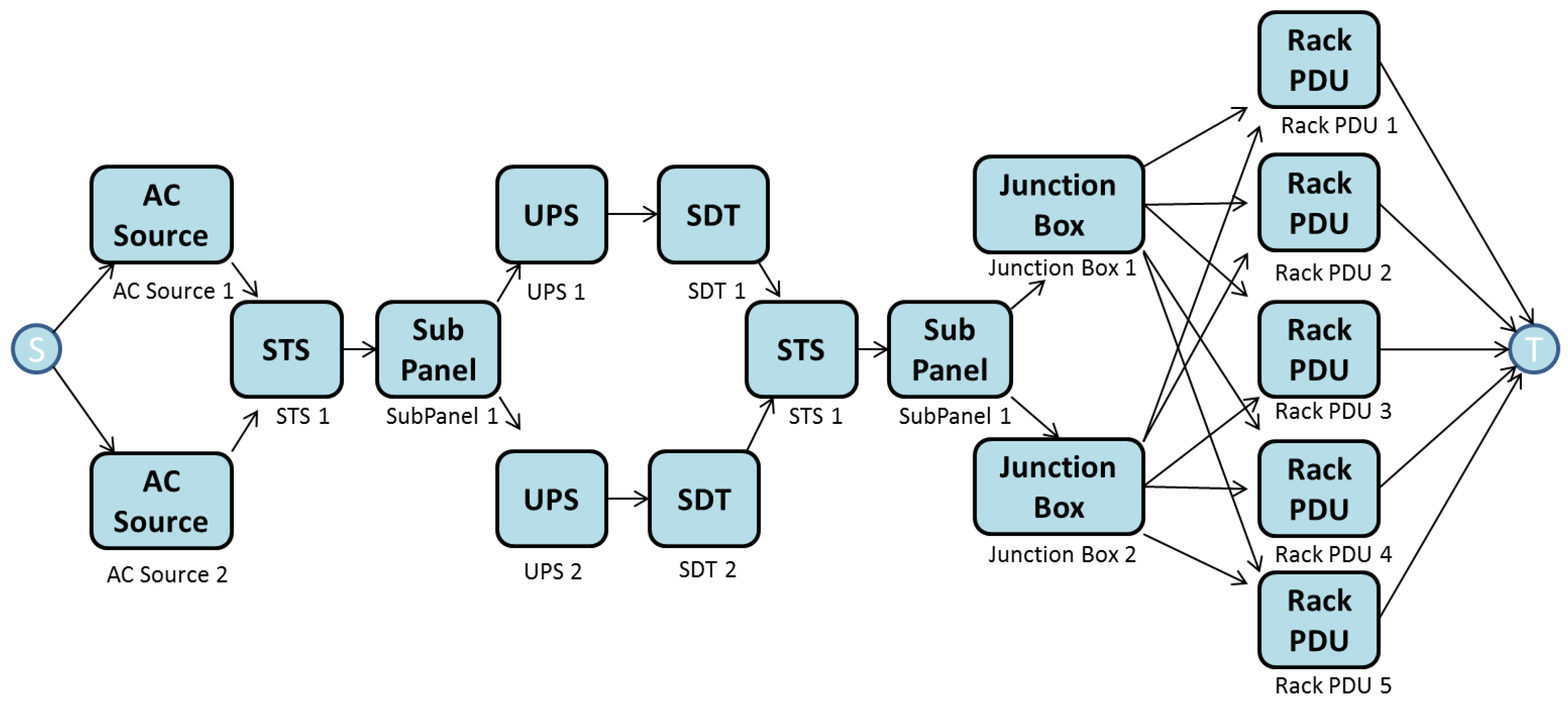
Once the availability is known, an EFM is created to compute a further set of metrics (e.g., cost and operational exergy) for each arrangement.
Figure 10 shows the EFM model for A5.
Figure 10.
Architecture A5 in the EFM model.
Figure 10.
Architecture A5 in the EFM model.
8.3. Results
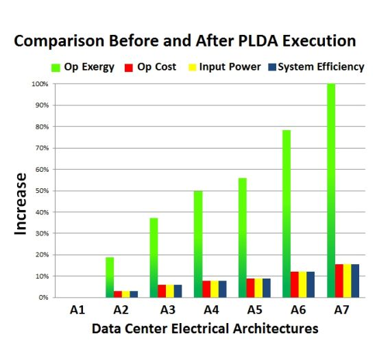
Table 4 summarizes the results for each power infrastructure, where A1 to A7 represent the architectures evaluated. Row
gives the results obtained before executing the PLDA; row
After is the results after PLDA execution;
Improvement (%) is the improvement achieved in percentage;
Op Exergy is the operational exergy in gigajoules (GJ);
Op Cost is the operational cost in UDS;
Availability is the availability level;
Number 9s is the availability in number of nines (−log[1−A/100]);
Downtime is the downtime cost per year;
Input Power is the input power in kW; and
System Efficiency is the system efficiency.
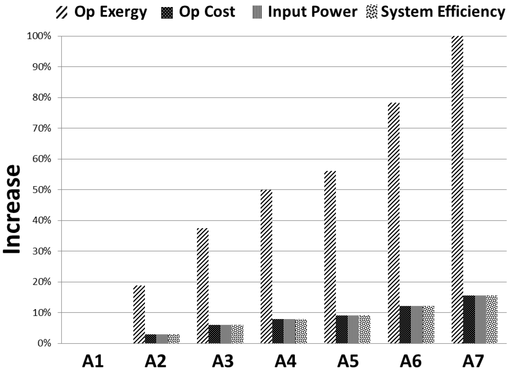
From the aforementioned table, the first thing to be noted is the improvement obtained. For instance, the operational cost of A7 is reduced by over 15% and the environmental impact by around 100%. Architecture A1 is the only architecture in which no improvement was observed. However, this behavior was expected, due to the absence of redundant devices.
Once higher levels of redundancy were adopted (considering devices with different efficiencies), better results were obtained with the PLDA algorithm. That fact is clearly evident in the graphical representation of the improvements obtained in all architectures, depicted in
Figure 11.
The PLDA does not affect the results of dependability. This behavior occurs, because with the EFM model, it is possible to compute operational exergy, operational cost, input power and system efficiency.
Table 4.
Results of PLDA execution with improvement in %.
Table 4.
Results of PLDA execution with improvement in %.
| Architectures | - | Op Exergy | Op Cost (USD) | Availability | Number 9s | Downtime (year) | Input Power | System Efficiency (%) |
|---|
| A1 | Before | 5,627 | 1,133,569 | 0.9979 | 2.684 | 18.121 | 1,178.82 | 84.82 |
| After | 5,627 | 1,133,569 | 0.9979 | 2.684 | 18.121 | 1,178.82 | 84.82 |
| Improvement (%) | 0 | 0 | 0 | 0 | 0 | 0 | 0 |
| A2 | Before | 6,922 | 1,174,589 | 0.9994 | 3.255 | 4.8667 | 1,219.63 | 81.99 |
| After | 5,823 | 1,140,993 | 0.9994 | 3.255 | 4.8667 | 1,184.75 | 84.4 |
| Improvement (%) | 18.8 | 2.9 | 0 | 0 | 0 | 2.9 | 2.9 |
| A3 | Before | 8,253 | 1,215,242 | 0.99943 | 3.25 | 4.92 | 1,261 | 79.24 |
| After | 6,010 | 1,146,719 | 0.99943 | 3.25 | 4.92 | 1,190 | 83.98 |
| Improvement (%) | 37.3 | 5.9 | 0 | 0 | 0 | 5.9 | 5.9 |
| A4 | Before | 9,005 | 1,238,130 | 0.9993 | 3.171 | 5.902 | 1,285 | 77.77 |
| After | 6,010 | 1,146,591 | 0.9993 | 3.171 | 5.902 | 1,190 | 83.98 |
| Improvement (%) | 49.8 | 7.9 | 0 | 0 | 0 | 7.9 | 7.9 |
| A5 | Before | 9,398 | 1,250,134 | 0.9993 | 3.172 | 5.8887 | 1,298 | 77.02 |
| After | 6,010 | 1,146,592 | 0.9993 | 3.172 | 5.8887 | 1,190 | 83.98 |
| Improvement (%) | 56 | 9 | 0 | 0 | 0 | 9 | 9 |
| A6 | Before | 10,383 | 1,280,685 | 0.9997 | 3.698 | 1.7547 | 1,329 | 75.22 |
| After | 5,825 | 1,141,398 | 0.9997 | 3.698 | 1.7547 | 1,184 | 84.4 |
| Improvement (%) | 78.2 | 12.2 | 0 | 0 | 0 | 12.2 | 12.2 |
| A7 | Before | 11,410 | 1,312,259 | 0.9999 | 5.11 | 0.067 | 1,361.84 | 73.43 |
| After | 5,639 | 1,135,910 | 0.9999 | 5.11 | 0.067 | 1,178 | 84.83 |
| Improvement (%) | 102 | 15.5 | 0 | 0 | 0 | 15.5 | 15.5 |
Figure 11.
Comparison before and after PLDA execution.
Figure 11.
Comparison before and after PLDA execution.
9. Conclusions
The present paper proposed an algorithm, called the Power Load Distribution Algorithm (PLDA), to reduce the electrical energy consumption of data center power infrastructures. The main goal of the PLDA algorithm is to automatically allocate more appropriate values to the edge weights of the EFM models. Such an optimization-based approach was evaluated through a case study, which demonstrated that the results obtained after the execution of the PLDA were significantly better. For some of the case study architectures, the results for sustainability impact (exergy) were improved by more than 100%, and power consumption, system efficiency and operational cost were improved by up to 15%. In the worst case, the results were equal to those obtained without the PLDA.
In the future, we intend to study how dynamic power management can help to optimize data center electrical consumption.


