4.1. Experimental Setup
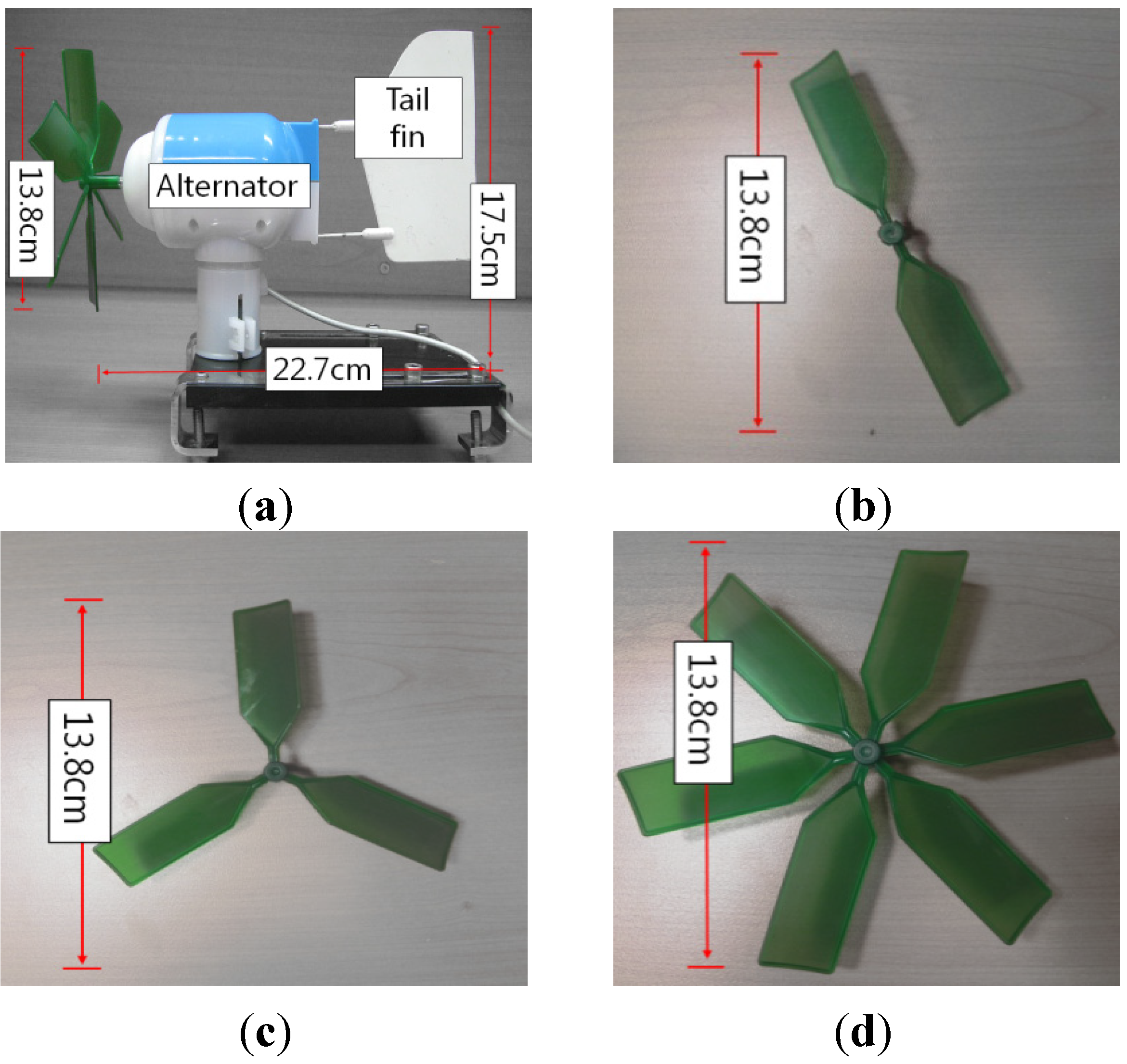
To verify the performance of the three micro-wind turbines (
i.e., the three horizontal-axis turbines in
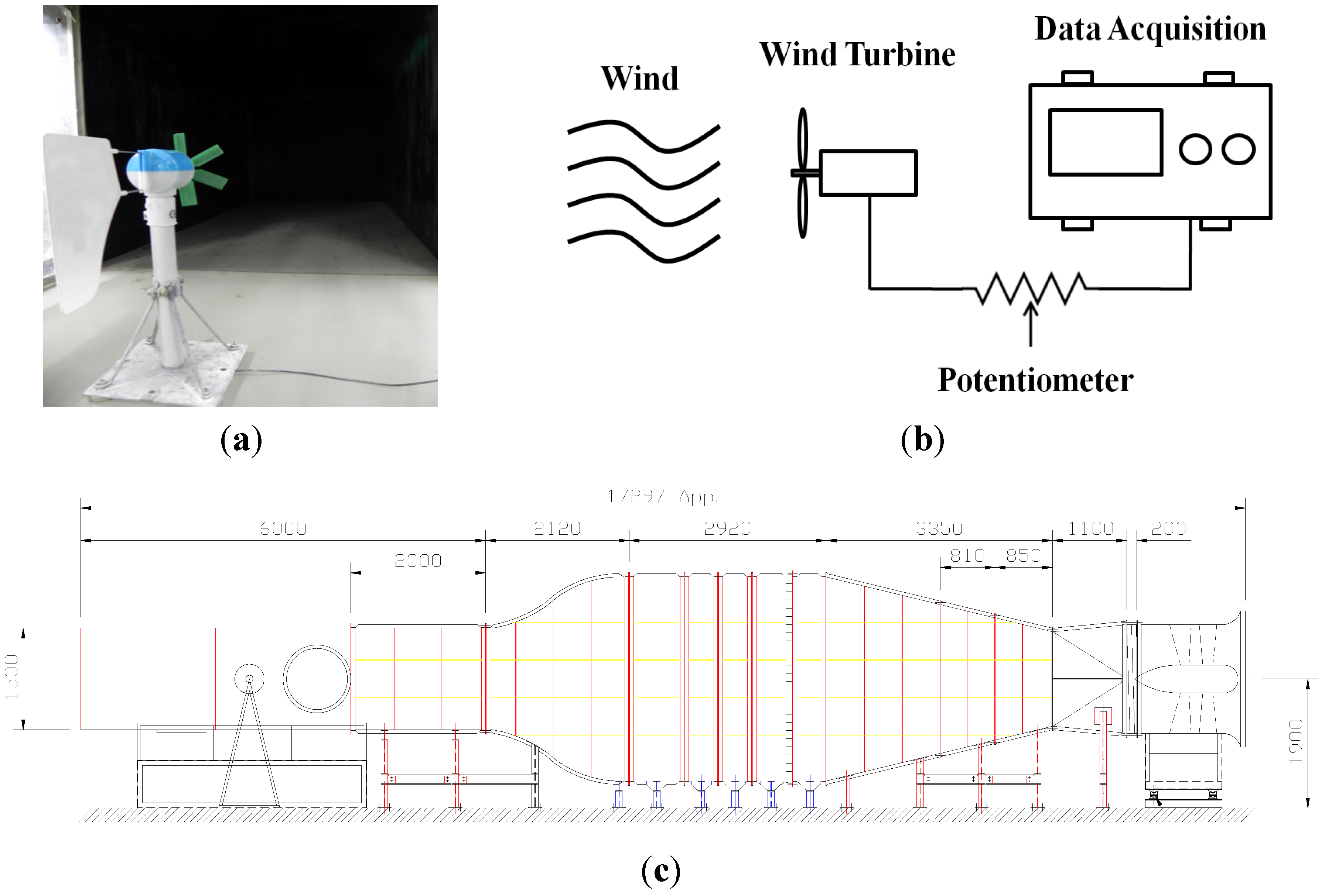
Figure 7), a series of the experimental tests was carried out in the wind tunnel with a constant wind speed. The dimensions of the wind tunnel used in this test are shown in
Figure 8(c). The power generated from the wind turbines passed through a potentiometer varying from 30 Ω to 5 kΩ that was used to tune the resistive loads; at each step, the output voltage from the wind turbines was measured by an oscilloscope, as shown in
Figure 8. The weather conditions for the ambient pressure, ambient temperature, and relative humidity in the laboratory were 995.5 hPa, 23 °C and 52%, respectively. Therefore, the air density was 1.1646 kg/m
3.
Figure 8.
Experimental setup: (a) wind turbine in the wind tunnel; (b) configuration of the experiment; (c) wind tunnel facility.
Figure 8.
Experimental setup: (a) wind turbine in the wind tunnel; (b) configuration of the experiment; (c) wind tunnel facility.
4.2. Experimental Results
The first experiment was done to evaluate the performance of the three different wind turbines under the same wind environment with an RMS wind speed of 7 m/s. The RPM (revolutions per minute) of the wind turbines was adjusted as the resistance of the potentiometer varied under the same wind environment and the output voltage at each load resistance step was measured.
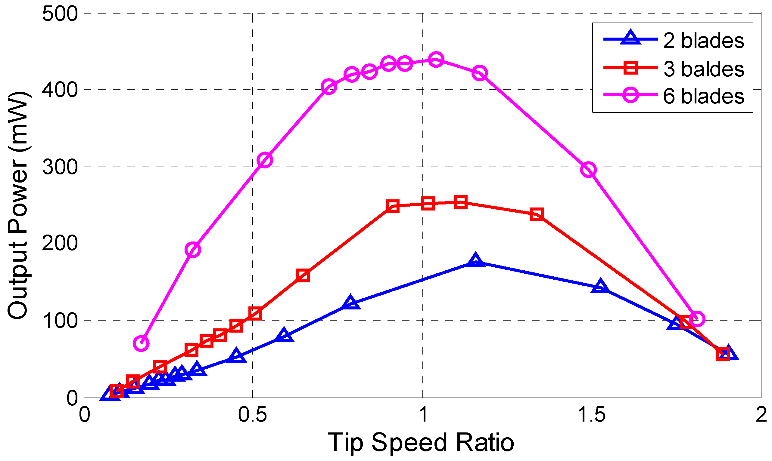
Figure 9 shows the RPM of the rotor
versus the output power with the three different types of rotors. Under the same wind speed, the RPM
versus the generated power for three-blade shapes are plotted by adjusting the resistance to find the maximum output power. From the result, it was demonstrated that the wind turbine with six-blade rotor had the most powerful performance, having a generated power of 439 mW with a wind speed of 7 m/s. In terms of the power density shown in
Table 5, the case with six blades also showed a maximum of 2.93 mW/cm
2, while the case with three showed 1.69 mW/cm
2 and that with two blades showed 1.17 mW/cm
2.
Figure 9.
Wind turbine efficiencies for three different types of rotors (at 7 m/s).
Figure 9.
Wind turbine efficiencies for three different types of rotors (at 7 m/s).
Table 5.
Output power with different type of rotors.
Table 5.
Output power with different type of rotors.
| Rotor type | Diameter (cm) | Maximum Output (mW) | Power Density (mW/cm2) |
|---|
| Two blades | 13.8 | 175.05 | 1.17 |
| Three blades | 13.8 | 252.80 | 1.69 |
| Six blades | 13.8 | 438.79 | 2.93 |
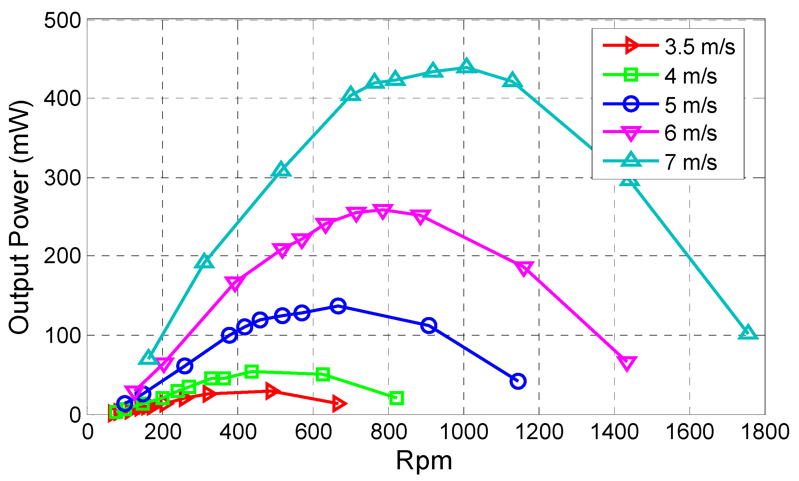
Next the performances under different wind speeds ranging from 3.5 m/s to 7 m/s were explored for the best performing six-blade rotor.
Figure 10 shows the evolution of the overall generated power of the wind turbine for five different wind speeds (
i.e., 3.5 m/s, 4 m/s, 5 m/s, 6 m/s and 7 m/s). For a wind speed of 3.5 m/s, which is the cut-in wind speed of the proposed wind turbine, a maximum of 28.88 mW power was achieved and a maximum power of 438.79 W at a wind speed of 7 m/s was obtained. The output voltage measurements at each maximum power point are summarized in
Table 6.
Figure 10.
Overall generated power of a micro-wind turbine with a six-blade rotor.
Figure 10.
Overall generated power of a micro-wind turbine with a six-blade rotor.
Table 6.
Outputs at the maximum power points.
Table 6.
Outputs at the maximum power points.
| Wind Speed (m/s) | Voltage (V) | Current (mA) | Power (mW) |
|---|
| 3.5 | 5.73 | 5.04 | 28.88 |
| 4 | 5.06 | 10.54 | 53.30 |
| 5 | 8.09 | 16.85 | 136.34 |
| 6 | 9.66 | 26.84 | 259.32 |
| 7 | 12.57 | 34.91 | 438.79 |
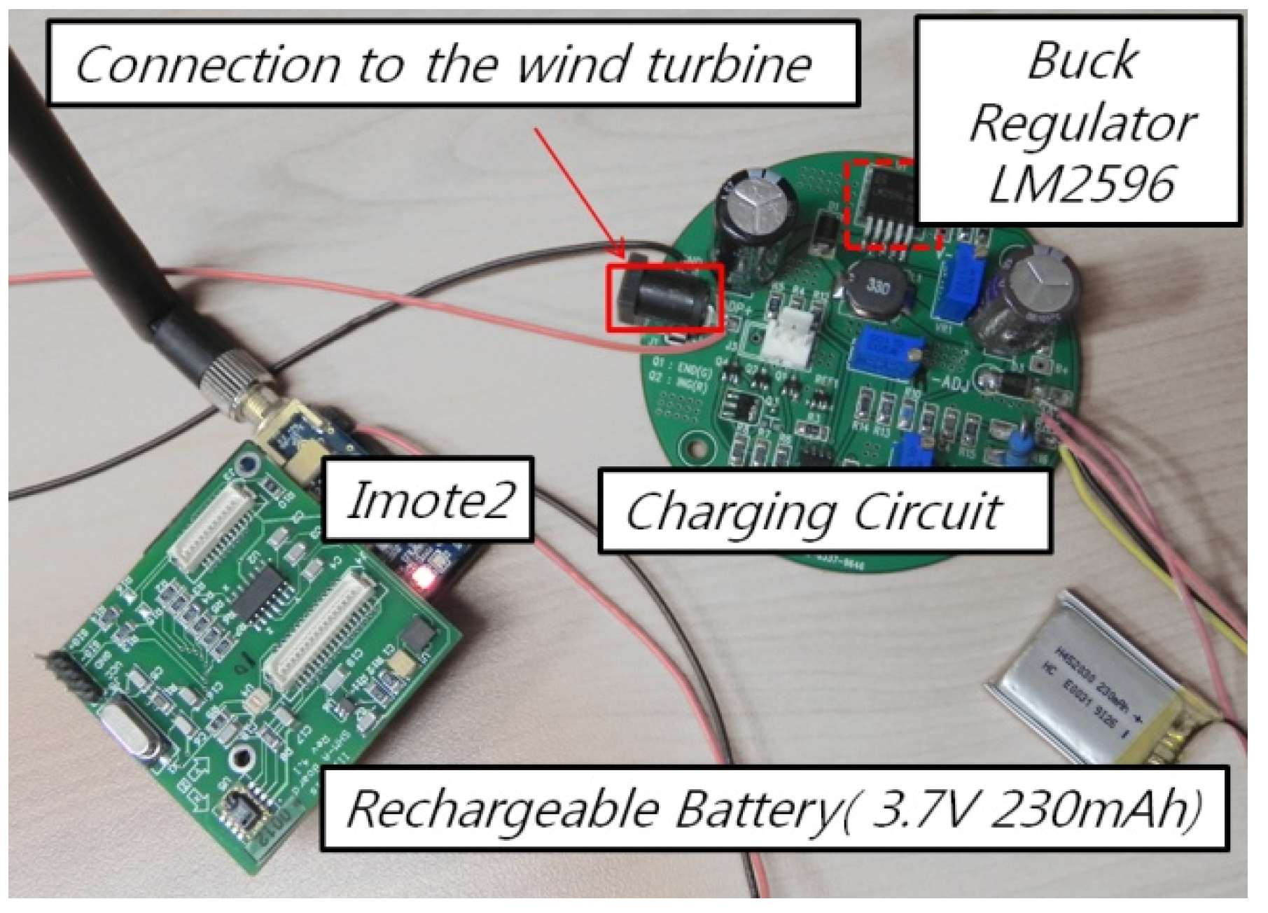
4.3. Validation of Self-Sufficient Operation Capacity
To test the feasibility of charging through the proposed wind turbine, it was connected to a rechargeable battery and a charging circuit as shown in
Figure 11. The main component of the charging circuit is a buck regulator (model LM2596). The LM2596 is a high-efficiency buck regulator that supports an input range of 7 V~30 V and an adjustable output range of 1.25 V~35 V. The output voltage of the LM2596 was set to 4.2 V to charge a Li-polymer rechargeable battery having a nominal voltage of 3.7 V, and a 230-mAh Li-polymer rechargeable battery was used.
Figure 11.
Charging system for the wireless sensor (Imote2).
Figure 11.
Charging system for the wireless sensor (Imote2).
The actual charging and sensing test was carried out with the same sensing parameters as done in
Table 3. The total power consumption during the test was 72.66 mWh as the power loss during the sleep mode (
i.e., 10 mWh) was excluded from the power consumption for one day in
Table 3.
In order to check the time required to recover the power loss during sensing, the wireless sensor node was equipped with the wind turbine and the charging circuit. Its result (
i.e., the “with charging” case) was compared with that of a sensor node without the turbine and the circuit (
i.e., the “without charging” case). Due to the limitation of the regulator and the impedance mismatch between the wind turbine and the charging circuit [
16], wind speeds lower than 7 m/s could not be used for the charging test.
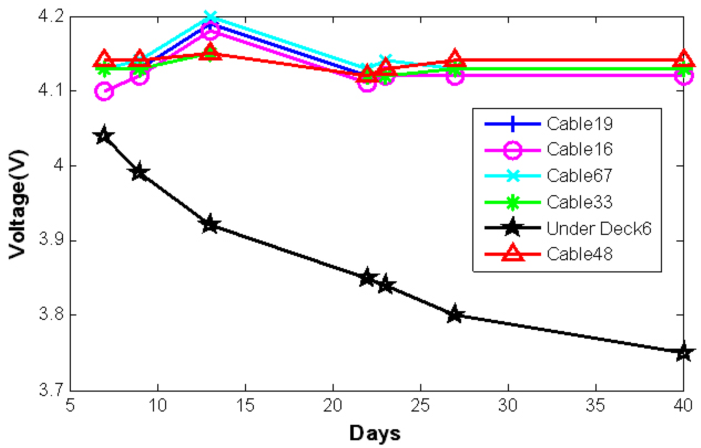
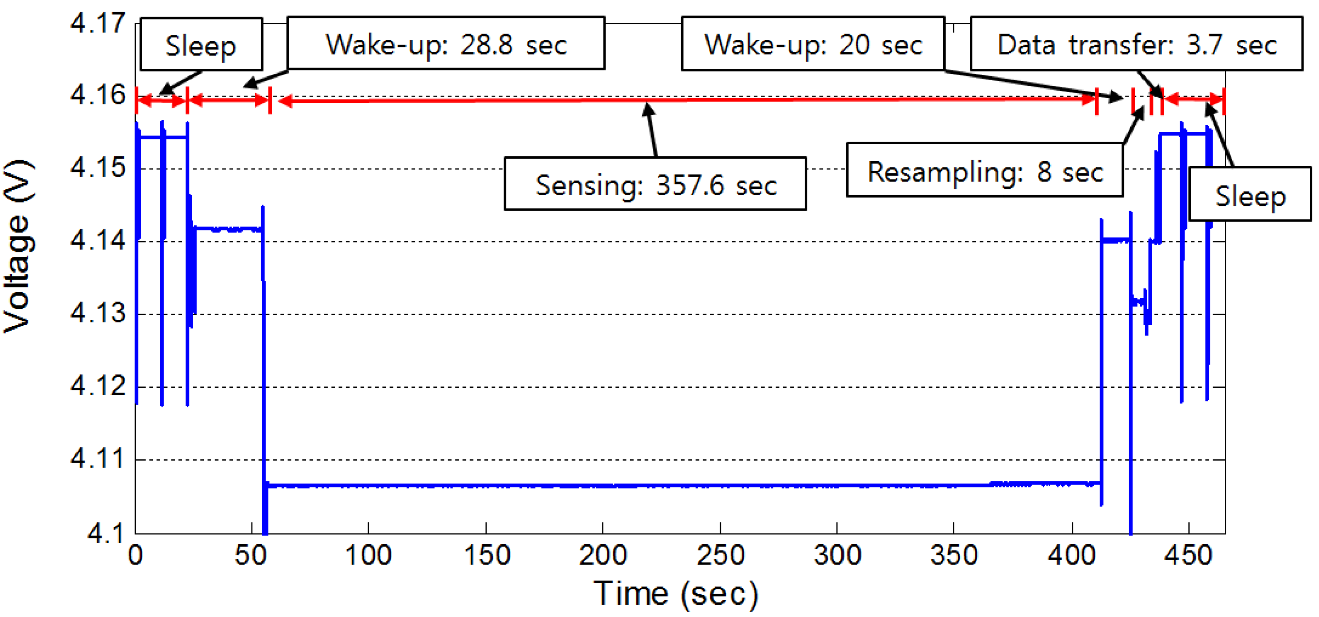
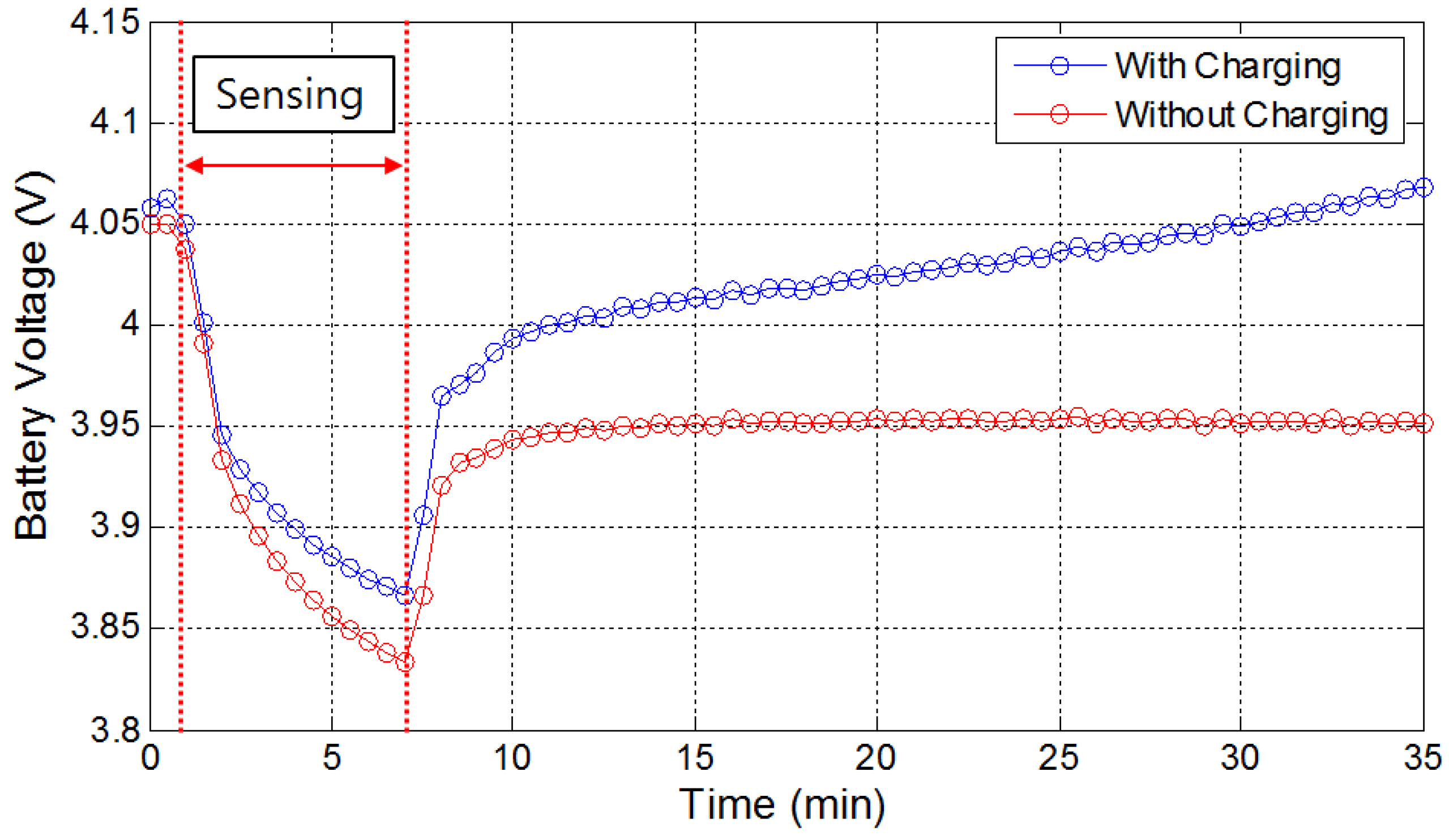
Figure 12 shows the battery voltage variations of two cases (
i.e., the “with charging” and the “without charging” cases) at a wind speed of 7 m/s. As shown in the figure, battery voltages in both cases declined rapidly during sensing due to the high level of power consumption. After sensing, the battery level in the “without charging” case had decreased, though it slightly recovered (
i.e., from 4.05 V to 3.95 V), showing a voltage drop of 0.1 V. In the ‘with charging’ case, the battery level during the sensing process showed a slight decrease; however, with charging from the wind turbine, the degree of the decline was more moderate, and showed a steadily increasing trend in terms of the battery level requiring a recovery time of 33 min.
Figure 12.
Battery levels according to the charging condition.
Figure 12.
Battery levels according to the charging condition.
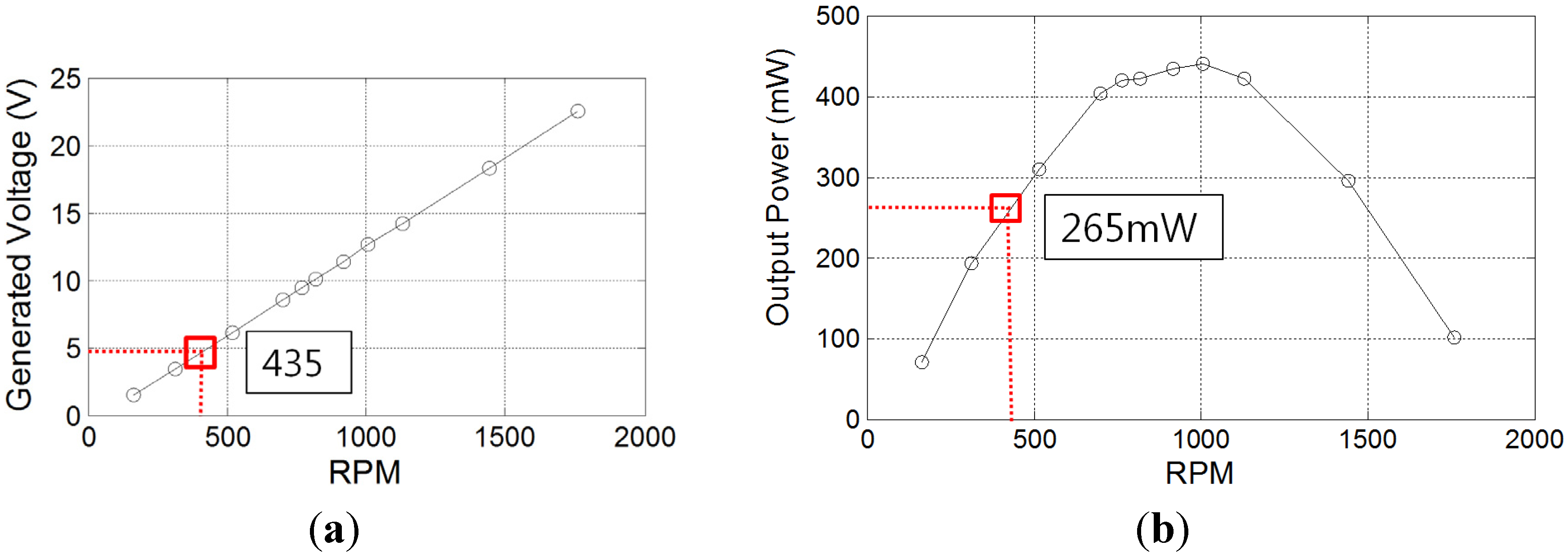
It was found from the actual power-charging test that the maximum power at 7 m/s (
i.e., 438.79 mW) was not extracted due to the impedance mismatch between the wind turbine and the charging circuit. The output voltage at the maximum power was 12.57 V, as shown in
Table 6; however, the voltage during the charging test from the charging circuit was 4.99 V. Under this impedance condition, the RPM was 435 rad/s and the corresponding generated output was 265 mW, as shown in
Figure 13.
Figure 13.
Output power and output voltage (at 7 m/s): (a) RPM versus the output voltage; (b) RPM versus the output power.
Figure 13.
Output power and output voltage (at 7 m/s): (a) RPM versus the output voltage; (b) RPM versus the output power.
Theoretically, 16.4 min is required to compensate for the power consumption of 72.66 mWh during the test (
i.e., 72.66 mWh/265 mW = 16.4 min). In practice, however, it took 33 min to recover the power loss completely. Therefore, the charging efficiency to the battery in this case was determined to be about 50%. If the maximum peak power [
16] can be extracted and the charging efficiency to battery is taken into account, it would take 19.8 min to recover the power loss. The maximum power can be harvested continuously through maximum power point tracking (MPPT) technique [
16,
17,
18] that tracks the peak power points of the power generating system for any given environmental conditions.
The charging time under different wind speeds was estimated and is summarized in
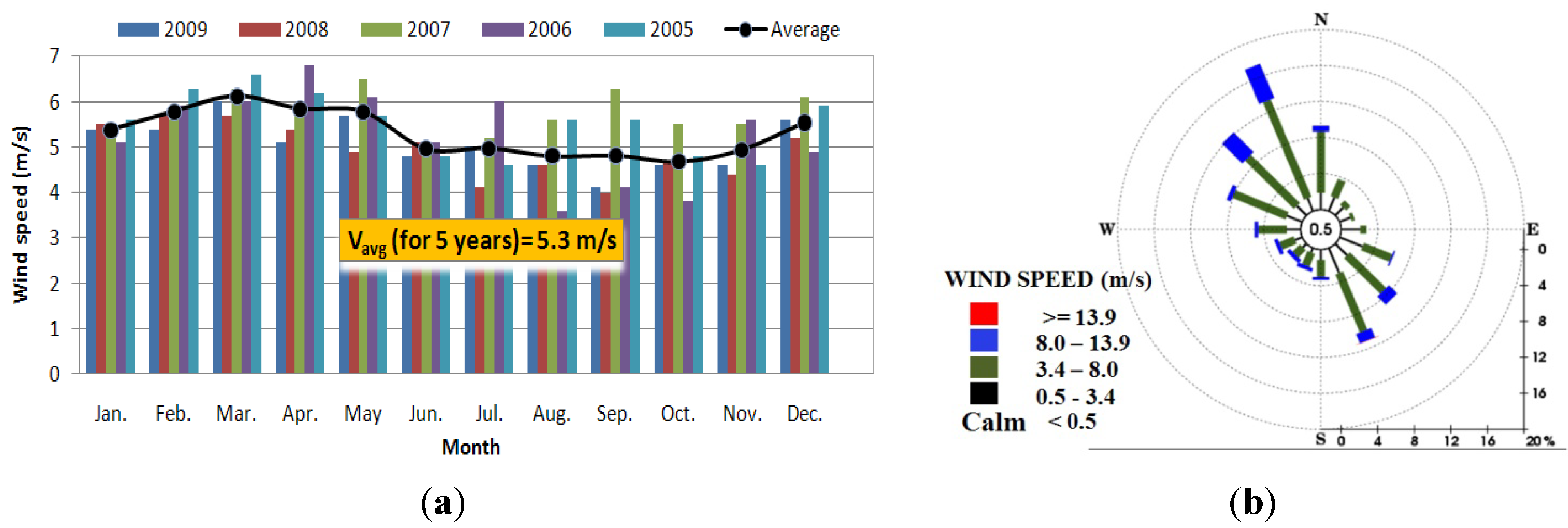
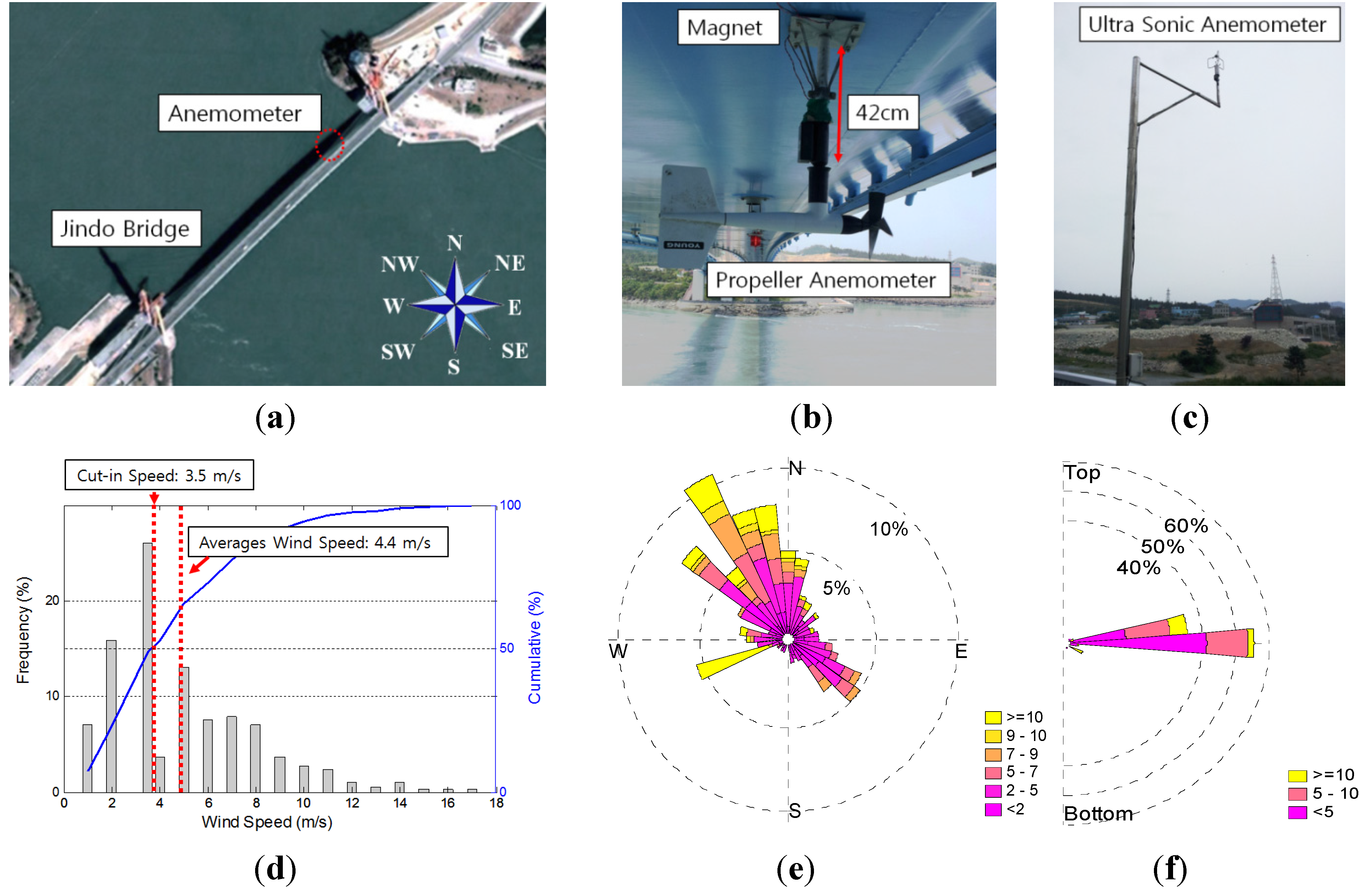
Table 7. Here, the charging efficiency to the battery for all the different wind speed cases is assumed to be identical, because the parameters affecting the charging efficiency, such as the charging method and the battery status, are almost the same for the different wind speeds. As seen from the table, there are large variations in the recovery time depending on the wind speed. At a wind speed of 7 m/s, only a short duration of wind of 19.8 min can operate the sensing process for a day, whereas 63.9 min and 163.4 min are required at a wind speed of 5 m/s and 4 m/s, respectively. It was found that a strong wind with a short duration was more efficient than a long-lasting low wind flow. Since the average wind speed at the Jindo Bridge site is 4.4 m/s and the cumulative wind distribution at 4 m/s is more than 50% (see
Figure 3(d)), wind blowing at 4 m/s or higher wind speed for 163.4 min (
i.e., about 2.7 h) is not a rare case. Moreover, the electricity generation process does not need to be continuous in this case. Even though the electricity is generated intermittently from the turbine, sufficient electrical energy can be ensured as long as the total electricity generation period is about 2.7 h in the case of 4 m/s or higher wind speed. This is quite feasible based on the wind measurement data from the Jindo Bridge site. Therefore, a wireless sensor with the proposed micro-wind turbine installed under the deck of the bridge may successfully perform the sensing process in most cases. However, if the proposed micro-wind turbine cannot provide the sufficient electricity for a stable functioning of the wireless sensor due to lacks of wind and electricity generation period for several consecutive low-wind days, combining a shadowed solar panel with the proposed wind turbine can be another alternative.
The efficiency of the proposed wind turbine varies from 7.50% to 14.25% for corresponding wind speeds of 3.5 m/s to 7 m/s as seen from
Table 7. This large amount of variation may result from friction in the generator, internal electrical resistance and efficiency of the rotors.
Table 7.
Estimated charging time.
Table 7.
Estimated charging time.
| Wind Speed (m/s) | Maximum Measured Power (mW) [A] | Recovery Time at Measured Power (min) | Available Wind Power (mW) [B] | Efficiency * (%) |
|---|
| 3.5 | 28.88 | 301.5 | 384.77 | 7.50 |
| 4 | 53.30 | 163.4 | 574.35 | 9.28 |
| 5 | 136.34 | 63.9 | 1121.78 | 12.15 |
| 6 | 259.32 | 33.6 | 1938.44 | 13.38 |
| 7 | 438.79 | 19.8 | 3078.18 | 14.25 |

