Mid-Term Energy Demand Forecasting by Hybrid Neuro-Fuzzy Models

Abstract

This paper proposes a structure for long-term energy demand forecasting. The proposed hybrid approach, called HPLLNF, uses the local linear neuro-fuzzy (LLNF) model as the forecaster and utilizes the Hodrick–Prescott (HP) filter for extraction of the trend and cyclic components of the energy demand series. Besides, the sophisticated technique of mutual information (MI) is employed to select the most relevant input features with least possible redundancies for the forecast model. Each generated component by the HP filter is then modeled through an LLNF model. Starting from an optimal least square estimation, the local linear model tree (LOLIMOT) learning algorithm increases the complexity of the LLNF model as long as its performance is improved. The proposed HPLLNF model with MI-based input selection is applied to the problem of long-term energy forecasting in three different case studies, including forecasting of the gasoline, crude oil and natural gas demand over the next 12 months. The obtained forecasting results reveal the noteworthy performance of the proposed approach for long-term energy demand forecasting applications.

1. Introduction

The world demand for energy is on a growing path due to the increase in world population. For instance, consumption of petroleum in the Unites States, as one of the world’s largest energy consumers, has increased by 20.4% from 1990 to 2005. The US natural gas consumption has also experienced a 16.32% increase within the same period [1]. Therefore, governments and policy-makers need accurate forecasts of energy demand, especially long-term forecasts, for large-scale decision making, such as investment planning for generation and distribution of energy.

Through the past decades, different methods have been developed for energy demand forecasting. The auto-regressive integrated moving average (ARIMA) model is one of the most popular time series-based methods which has been used for energy consumption prediction to a great extent. For instance, Haris and Liu proposed ARIMA and transfer function models for prediction of electricity consumption [2]. ARIMA and seasonal ARIMA (SARIMA) were used by Ediger and Akar to estimate the future primary energy consumption of Turkey from 2005 to 2020 [3]. Linear regression models have also been proposed for energy consumption prediction [4].

However, when nonlinearity of the forecasting problem prevails, the linear approaches may fail to capture the nonlinear dynamics of the process. In the past decade, computational intelligence (CI)-based models have been at the center of attention in forecasting applications, such as energy consumption and demand forecasting. The CI-based methods can effectively capture and model the nonlinear behavior of time series. Fuzzy logic and artificial neural networks (ANN) are two main CI-based techniques which have found many applications in modeling and prediction. Energy consumption modeling and forecasting are also among the applications of the CI-based approaches. Azadeh et al. estimated the oil demand in the US, Canada, Japan and Australia using a fuzzy regression modeling approach [5]. A hybrid technique of well-known Takagi-Sugeno fuzzy inference system and fuzzy regression has been proposed for prediction of short-term electric demand variations by Shakouri et al. [6]. In their study, they proposed a type III TSK fuzzy inference machine combined with a set of linear and nonlinear fuzzy regressors in the consequent part to model the effects of climate change on the electricity demand. Padmakumari et al. combined neural network and fuzzy modeling for long-term distribution load forecasting [7]. They employed radial basis function network (RBFN) as the neural network part of their approach. Long-term monthly gasoline demand forecasting has been performed using an intelligent adaptive algorithm in [8]. The intelligent algorithm, composed of artificial neural network, conventional regression and design of experiment (DOE), was applied for monthly gasoline demand forecasting in Japan, USA, Kuwait, Canada and Iran. Based on the findings in [8], ANN provides far less error than regression. Yokoyama et al. concentrated on neural networks to predict energy demands [9]. They used an optimization technique, termed “Modal Trimming Method” to optimize model’s parameters and then forecasted cooling demand in buildings. A considerable number of review studies on intelligent demand forecasting, have also been published. A comprehensive literature survey on electric demand forecasting using artificial intelligence (AI) techniques has been presented in [10]. This literature review study has presented a wide-range biography of numerous papers, concentrated on AI-based load forecasting techniques such as expert systems, fuzzy, genetic algorithm, artificial neural network (ANN), etc. Another review on electric load forecasting approaches has been conducted by Hahn et al. in [11]. They have provided an overview on classical time series and regression methods as well as artificial intelligence and computational intelligence approaches. Various traditional and CI-based models for energy demand forecasting have been also reviewed in [12].

Due to successful application of the neural networks and fuzzy inference systems, the synergistic combination of them, i.e., neuro-fuzzy models, have also been proposed for energy consumption prediction. For instance, Chen proposed a fuzzy-neural approach for long-term forecasting of electric energy in Taiwan [13]. As another example, the adaptive neuro-fuzzy inference system (ANFIS) has been employed for short-term forecasting of natural gas demand [14]. In this research, the ANFIS approach was used with pre-processing and post-processing techniques to enhance forecasting accuracy. Nostrati et al. also proposed a neuro fuzzy model for long- term electrical load forecasting [15].

In this paper, we develop a long-term energy demand forecasting approach established on the HP filtering, MI-based input selection and LLNF modeling. Due to the high correlation of the energy demand series to the population, such series often contain a trend component. Hence using HP filter for decomposition of the demand time series into trend and cyclic components is proposed as an effective technique for energy demand forecasting. Since the energy demand series are affected by various factors such as population, GDP as well as demand historical, selection of the most appropriate inputs turns to be a challenging task. As another novelty behind this paper, we employ the sophisticated technique of mutual information for selection of the inputs with most relevance to the output and the least redundancy and enhancing the modeling performance of the LLNF model to a considerable extent. Finally, after presenting the mathematical description of the mentioned techniques, the proposed HPLLNF + MI approach is implemented in three case studies for forecasting long-term demand of gasoline, crude oil and natural gas in the United States.

2. Framework of the Forecasting Approach

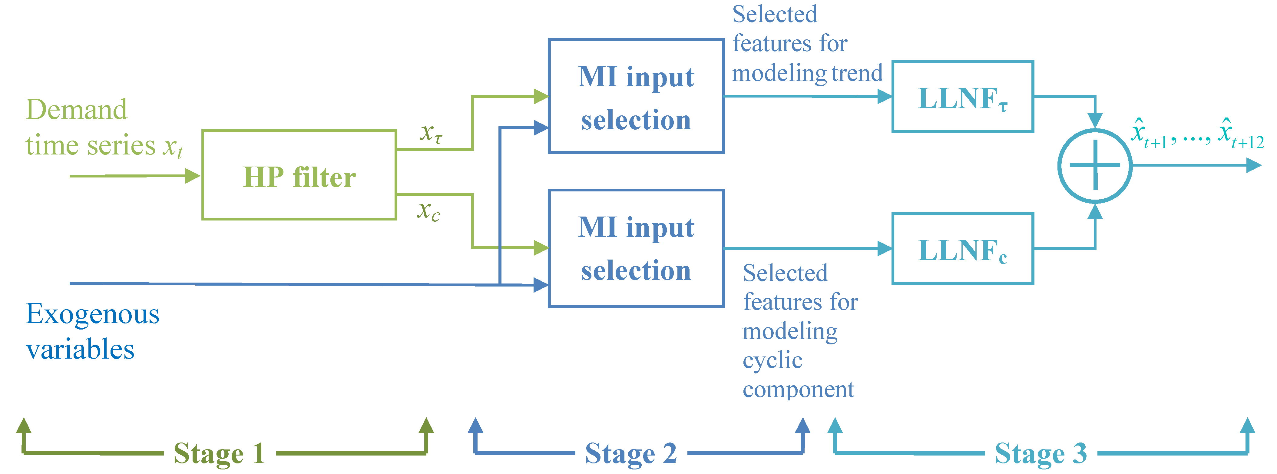
A general description of our proposed energy demand forecast framework is presented in this section. In brief, the proposed approach includes three stages: data preprocessing, input selection and forecasting, as shown by Figure 1.

Figure 1. Structure of the proposed forecasting approach.

Figure 1. Structure of the proposed forecasting approach.

In the first stage, the time series of energy demand up to the test period is passed through the HP filter and trend and cyclic components are generated. This decomposition allows us to model trend and fluctuations of the time series separately and more accurately. It must be noted that trend and cyclic components are separately modeled by LLNF_τ and LLNF_c, respectively. Then, in the next stage, the input selection technique of mutual information is employed to determine appropriate inputs for each of LLNF models. In the third stage, the selected input variables are applied to LLNF models and forecast values are provided. By aggregating the predictions of the two LLNF models, final values of the energy demand forecast are produced.

3. Local Linear Neuro-Fuzzy Models

A neuro-fuzzy (NF) model is a fuzzy system drawn in a neural network structure, combining the learning, parallel processing and generalization capabilities of neural networks and logicality, transparency and use of a priori knowledge in fuzzy systems. A local linear neuro-fuzzy system, as a notable category of NF models, decomposes an a priori unknown global nonlinear system into a series of local linear models and then tries to carry out the simpler task of identifying parameters of linear sub-models [16,17].

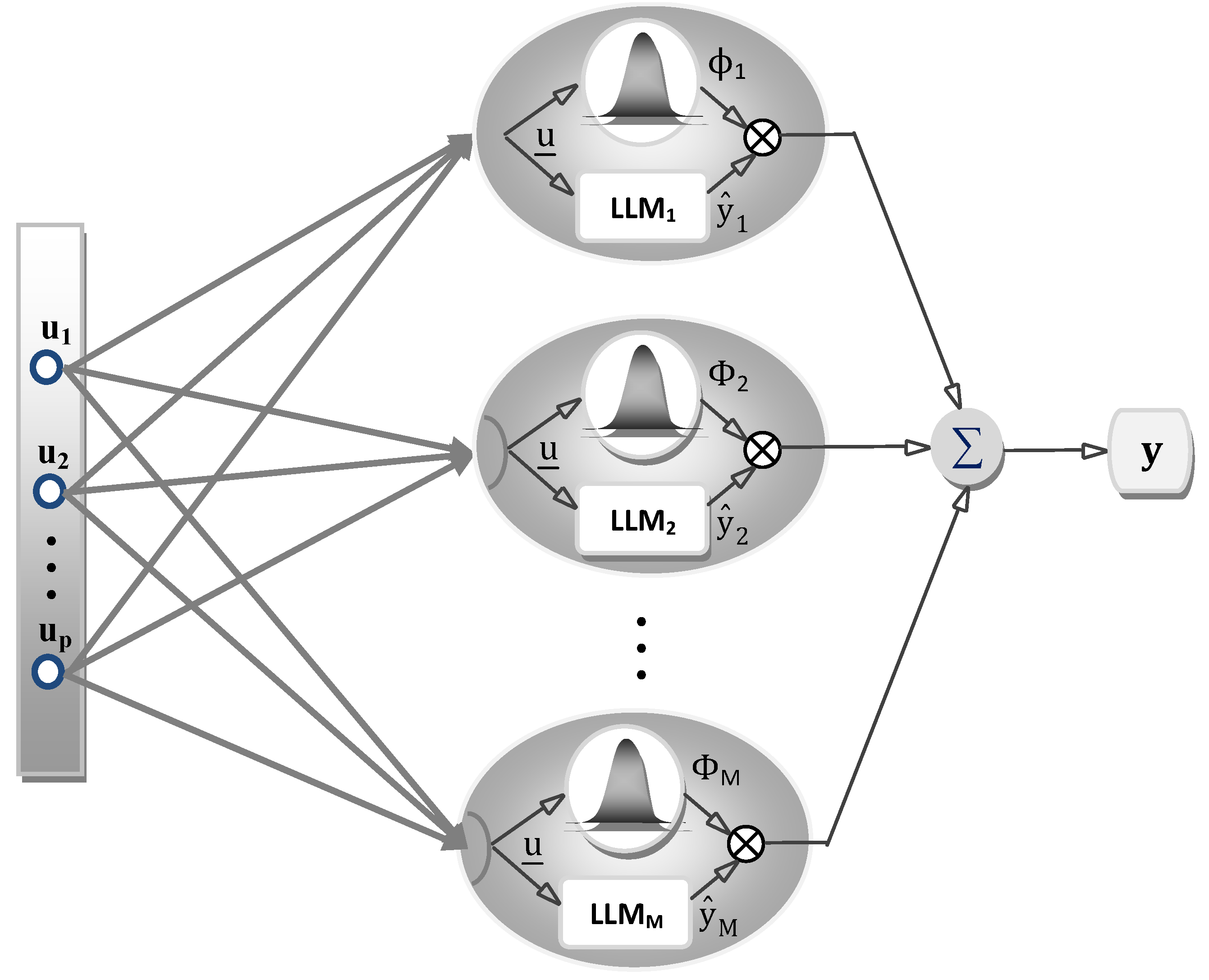
The network structure of a LLNF model is illustrated by Figure 2. In LLNF model, each neuron is composed of a local linear model (LLM) and a validity function which sets the validity region of the LLM. Accordingly, for input vector $\underset{\_}{u}={\left[u_1{u}_2\cdots u_p\right]}^T$, the unknown nonlinear system can be approximated in the following form:

$$\widehat{y}={\displaystyle \sum _{i=1}^M{\widehat{y}}_i{\varphi }_i\left(\underset{\_}{u}\right)}$$

(1)

which is an interpolation of M local sub-models, weighted with validity functions ${\varphi }_i$.

The output of each LLM (${\widehat{y}}_i$) can be stated as follows:

$${\widehat{y}}_i={\theta }_{i0}+{\theta }_{i1}{u}_1+{\theta }_{i2}{u}_2+\mathrm{...}+{\theta }_{ip}{u}_p$$

(2)

where θ_ij are LLM parameters associated with neuron i.

In order to ensure that contribution of all local sub-models amounts to 100%, the validity functions are normalized to form a partition of unity, i.e.,

$${\displaystyle \sum _{i=1}^M{\varphi }_i\left(\underset{\_}{u}\right)=1}$$

(3)

with validity functions ${\mu }_j\left(\underset{\_}{u}\right)$, which are not normalized, the normalized validity functions ${\varphi }_j\left(\underset{\_}{u}\right)$, can be computed using the following:

$${\varphi }_i\left(\underset{\_}{u}\right)=\frac{{\mu }_i\left(\underset{\_}{u}\right)}{{\displaystyle \sum _{j=1}^M{\mu }_j\left(\underset{\_}{u}\right)}}$$

(4)

Figure 2. Structure of the LLNF model.

Figure 2. Structure of the LLNF model.

In the presented description of the LLNF model, two types of parameters should be identified; the parameters associated with local linear models (θ_ij) and the parameters associated with validity functions. The former parameters are called rule consequent parameters, while the latter are referred to as rule premise parameters.

Global and local estimation procedures can be employed for the identification of the parameters of the local linear models. It is shown that for low noise level, the global estimation outperforms the local approach. Furthermore, the former has better interpolation behavior. However, the local estimation performs better for high noise level and has less computational complexities [16]. Both of these approaches will be considered in this paper. The sophisticated local linear model tree (LOLIMOT) algorithm is also utilized for identification of the validity functions parameters.

3.1. Global Estimation of the Local Linear Models Parameters

A single least-square algorithm is run for global estimation of rule consequent parameters. Hence the following least squares optimization enters the problem:

$$\underset{\underset{\_}{\theta }}{\min }I={\displaystyle \sum _{j=1}^{N}e\left(j\right)}$$

(5)

where $e\left(j\right)=y\left(j\right)-\widehat{y}\left(j\right)$ and $\underset{\_}{y}={\left[y\left(1\right)y\left(2\right)\cdot \cdot \cdot y\left(N\right)\right]}^T$ contains the measured outputs.

For an LLNF model with M neurons and P inputs, the vector of linear parameters contains $n=M\left(p+1\right)$ elements:

$$\underset{\_}{\theta }=[{\theta }_{10}{\theta }_{11}\mathrm{...}{\theta }_{1p}{\theta }_{20}{\theta }_{21}\mathrm{...}{\theta }_{2p}{\theta }_{M0}{\theta }_{M1}\mathrm{...}{\theta }_{Mp}]{}^T$$

(6)

The corresponding regression matrix $\underset{\_}{X}$ for N measured data samples is:

$$\underset{\_}{X}=\left[{\underset{\_}{X}}_1{\underset{\_}{X}}_2\mathrm{...}{\underset{\_}{X}}_M\right]$$

(7)

where the regression sub-matrix ${\underset{\_}{X}}_i$ takes the following form:

$$\left[\begin{array}{cccc}{\varphi }_i\left(\underset{\_}{u}\left(1\right)\right)& u_1\left(1\right){\varphi }_i\left(\underset{\_}{u}\left(1\right)\right)& \mathrm{...}& u_p\left(1\right){\varphi }_i\left(\underset{\_}{u}\left(1\right)\right)\\ {\varphi }_i\left(\underset{\_}{u}\left(2\right)\right)& u_1\left(2\right){\varphi }_i\left(\underset{\_}{u}\left(2\right)\right)& \mathrm{...}& u_p\left(2\right){\varphi }_i\left(\underset{\_}{u}\left(2\right)\right)\\ ⋮& ⋮& & ⋮\\ {\varphi }_i\left(\underset{\_}{u}\left(N\right)\right)& u_1\left(N\right){\varphi }_i\left(\underset{\_}{u}\left(N\right)\right)& \mathrm{...}& u_p\left(N\right){\varphi }_i\left(\underset{\_}{u}\left(N\right)\right)\end{array}\right],i=1,\mathrm{...},M$$

(8)

Hence:

$$\underset{\_}{\widehat{y}}=\underset{\_}{X}.\underset{\_}{\widehat{\theta }};\underset{\_}{\widehat{\theta }}={\left({\underset{\_}{X}}^T\underset{\_}{X}\right)}^{-1}{\underset{\_}{X}}^T\underset{\_}{y}$$

(9)

3.2. Local Estimation of the Local Linear Models Parameters

While all $n=M\left(p+1\right)$ of the local linear models are estimated simultaneously by the global estimation approach, in the local approach M separate local estimations are performed for the $p+1$ parameters of each local linear model. The parameter vectors for each of the estimations are:

$${\underset{\_}{\theta }}_i={\left[{\theta }_{i0}{\theta }_{i1}\mathrm{...}{\theta }_{ip}\right]}^T,i=1,\mathrm{...},M$$

(10)

The corresponding regression matrices are:

$${\underset{\_}{X}}_i=\left[\begin{array}{cccc}1& u_1\left(1\right)& \mathrm{...}& u_p\left(1\right)\\ 1& u_1\left(2\right)& \mathrm{...}& u_p\left(2\right)\\ ⋮& ⋮& & ⋮\\ 1& u_1\left(N\right)& \mathrm{...}& u_p\left(N\right)\end{array}\right],i=1,\mathrm{...},M$$

(11)

It must be noted that all local linear models have identical regression matrix, since the elements of the ${\underset{\_}{X}}_i$ do not depend on i. The output of each local linear model is valid in the region where the corresponding validity function is close to unity. Hence, as the validity function decreases, the data become less relevant for estimation of ${\underset{\_}{\theta }}_i$. Therefore, the validity function values are introduced as weighting factors in the error function to carry out a weighted least squares optimization:

$$\underset{{\underset{\_}{\theta }}_i}{\min }{I}_i={\displaystyle \sum _{j=1}^N{\varphi }_i\left(\underset{\_}{u}\left(j\right)\right)e\left(j\right)}$$

(12)

The solution for the weighted least squares problem in (11) is given below:

$${\underset{\_}{\theta }}_i={\left({\underset{\_}{X}}_i^T{\underset{\_}{Q}}_i{\underset{\_}{X}}_i\right)}^{-1}{\underset{\_}{X}}_i^T{\underset{\_}{Q}}_i\underset{\_}{y}$$

(13)

where ${\underset{\_}{Q}}_i$ is the N × N diagonal weighting matrix:

$${\underset{\_}{Q}}_i=\left[\begin{array}{cccc}{\varphi }_i\left(\underset{\_}{u}\left(1\right)\right)& 0& \mathrm{...}& 0\\ 0& {\varphi }_i\left(\underset{\_}{u}\left(2\right)\right)& \mathrm{...}& 0\\ ⋮& ⋮& & ⋮\\ 0& 0& \mathrm{...}& {\varphi }_i\left(\underset{\_}{u}\left(N\right)\right)\end{array}\right]$$

(14)

3.3. Estimation of the Validity Functions Parameters

The local linear model tree algorithm is used for estimation of validity functions parameters. This algorithm, owing to its fast rate of convergence, computational efficiency and intuitive constructive implementation is preferred to other optimization methods such as genetic algorithms and simulated annealing. The LOLIMOT algorithm utilizes multivariate normalized axis-orthogonal Gaussian membership functions, as stated below:

$$\begin{array}{ll}{\mu }_i\left(\underset{\_}{u}\right)& =\exp \left(-\frac{1}{2}\left(\frac{{\left(u_1-c_{i1}\right)}^2}{{\sigma }_{i1}^2}+\mathrm{...}+\frac{{\left(u_p-c_{ip}\right)}^2}{{\sigma }_{ip}^2}\right)\right)\\ & =\exp \left(-\frac{1}{2}\frac{{\left(u_1-c_{i1}\right)}^2}{{\sigma }_{i1}^2}\right)\cdot \mathrm{...}\cdot \exp \left(-\frac{1}{2}\frac{{\left(u_1-c_{i1}\right)}^2}{{\sigma }_{i1}^2}\right)\end{array}$$

(15)

where c_ij and σ_ij represent center coordinate and standard deviation of normalized Gaussian validity function associated with ith local linear model. The validity functions in (15) are normalized according to (4).

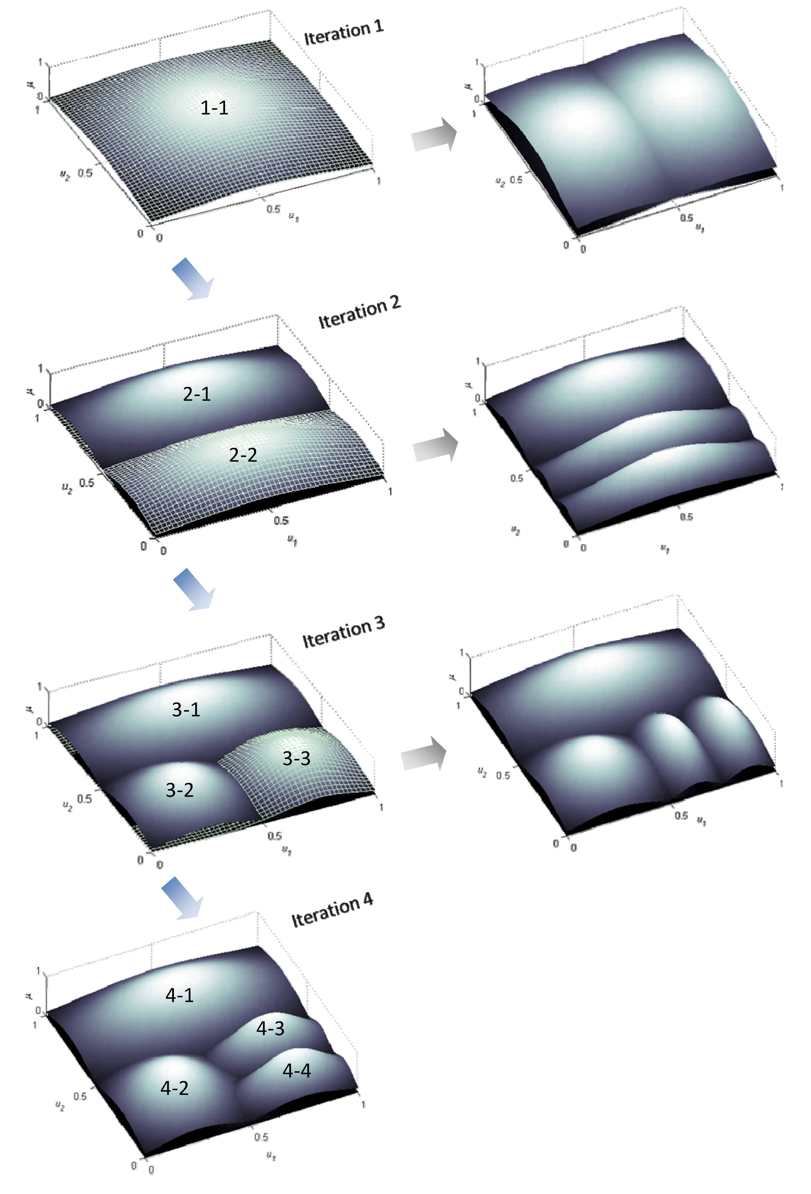
In the LOLIMOT algorithm, the input space is divided into hyper-rectangles by axis-orthogonal cuts based on a tree structure. Each hyper-rectangle represents an LLM. At each iteration, the LLM with worst performance is divided into two halves. Then Gaussian membership functions are placed at the centers of the hyper-rectangles and standard deviations are selected proportional to the extension of hyper-rectangles (usually 1/3 of hyper-rectangle’s extension). This procedure is summarized below:

• Start with the initial model: Set M = 1 and start with a single LLM whose validity function (${\varphi }_1\left(\underset{\_}{u}\right)$) covers the whole input space.
• Find the worst LLM: Calculate a loss function, here RMSE, for each of i = 1,2,…,M, LLMs and find the worst LLM.
• Check all divisions: The worst LLM, in all of p-dimensions, must be divided into two equal halves. For each of p divisions, a multidimensional validity function must be constructed for both new hyper-rectangles, then the rule consequent parameters of both new LLMS must be estimated using global/local least squares approach and finally the loss function for the current overall model must be computed.
• Find the best division: The best LLM related to the lowest loss function value, must be determined. The number of LLMS is incremented: M → M + 1. If the termination criterion, e.g., a desired level of validation error or model’s complexity, is met then stop, otherwise go to step 2.

Maximum generalization and noteworthy forecasting performance are among the salient features of the model identified by LOLIMOT learning algorithm. A three-dimensional graphical representation of partitioning of a two-dimensional input space by LOLMOT using up to four iterations is illustrated by Figure 3.

Figure 3. Operation of LOLIMOT in the first four iterations in a two-dimensional input space.

Figure 3. Operation of LOLIMOT in the first four iterations in a two-dimensional input space.

4. Data Pre-Processing Using a Hodrick-Prescott Filter

Data pre-processing often leads to desirable results in the field of system modeling, estimation and prediction. Application of data processing techniques in time series prediction is a recently introduced field of study mainly focusing on extracting useful information from available data and eliminating useless and ineffective information. Removal of high-frequency and noisy components of the time series by an appropriate filtering approach, results in a smoothed, well-behaved, and more predictable series.

The Hodrick-Prescott (HP) filter, introduced by Hodrick and Prescott, is a mathematical tool for extracting trend and cyclic components of a time series [18]. The HP filter is widely used in macroeconomic time series modeling [19,20]. Combination of HP filter and CI based techniques has also been proposed. For instance, in [21] Li and Huicheng used a HP filter and fuzzy neural networks to forecast urban water demand. They decomposed the factors correlative with the water demand into trend and cyclic components. Then multiple linear regression and fuzzy neural network were employed to forecast the trend and cyclic components of the correlative factors, respectively. It must be noted that in the presented approach in [21], separate models must be developed for each influencing factor, which increases complexity of the approach if there are many influencing factor.

The idea behind the HP filter technique is to break down a given time series into a trend component and a cyclic component. Consider that time series $h\left(t\right)$ is composed of trend and cyclic component:

$$h\left(t\right)=\tau \left(t\right)+c\left(t\right)$$

(16)

where $\tau$ and $c$ are trend and cyclic components, respectively. The HP filter removes the cyclic component by the following minimization problem:

$$\min \left\{{\displaystyle \sum _{t=1}^T{\left(h\left(t\right)-\tau \left(t\right)\right)}^2+\lambda {\displaystyle \sum _{t=2}^{T-1}{\left[\left(\tau \left(t+1\right)-\tau \left(t\right)\right)-\left(\tau \left(t\right)-\tau \left(t-1\right)\right)\right]}^2}}\right\}$$

(17)

where T is the length of the time series. The first term in (17) determines the fitness of the time series, while smoothness is controlled by the second term. A compromise between the fitness and the smoothness can be made through multiplier $\lambda$. This factor must be determined based on the frequency of the data. For $\lambda =0,$ the trend component is identical to the original series. The larger the value of $\lambda$, the higher smoothness is achieved. The value $\lambda =14400$ has been suggested in literature for monthly data [18]. The cyclic component of $c$ is obtained by subtracting the trend component $\tau$, from the original time series.

We employ the HP filter to decompose the original demand series to its trend and cyclic components. Then separate LLNF models are used for predicting each component. The final predictions are obtained by aggregating predicted values for trend and cyclic components. It’s worth noting that in comparison to the approach presented in [21], we develop an LLNF model for the trend component as well, which can bring about satisfactory results due to generalizability of the LOLIMOT learning algorithm. Furthermore, only two LLNF models are used to build the forecast model.

5. Mutual Information-Based Input Selection

Apart from the modeling approach employed, the input selection technique considerably affects prediction accuracy. Building the forecast model based on the irrelevant or unnecessary input variables may adversely influence the model’s performance. Using insufficient input variables leads to a model which is unable to capture the dynamics of the target system. On the other hand, employing a large number of unnecessary input variables exposes the model to the phenomenon of over-fitting. Hence, adopting an appropriate input selection technique is of utmost importance in prediction applications. Correlation analysis, Principal component analysis and mutual information (MI) are input selection techniques, used by researchers [22,23]. The first two methods are linear techniques which perform poorly when nonlinear relationships between input variables prevail. On the other hand, mutual information, as a measure of dependencies, is very powerful in assessing the relevance or redundancy of the input variables [24]. In this paper, we employ MI techniques to select appropriate inputs for energy demand forecasting.

5.1. Definition of Mutual Information

The concept of MI, originated from Shannon entropy, addresses the dependencies between random variables [24]. The MI between two random variables X and Y expresses the amount of information shared by them. In other words, the MI between X and Y measures the reduction in uncertainty on X due to the knowledge provided by Y and vice versa [24]. The MI between random variables X and Y, $I\left(X,Y\right)$, is defined by:

$$\begin{array}{ll}I\left(X,Y\right)& =H\left(X\right)-H\left(X|Y\right)\\ & =H\left(Y\right)-H\left(Y|X\right)\\ & =H\left(X\right)+H\left(Y\right)-H\left(X,Y\right)\end{array}$$

(18)

where, $H\left(X\right)$ and $H\left(Y\right)$ are entropies of X and Y, $H\left(X|Y\right)$ and $H\left(Y|X\right)$ are conditional entropies and $H\left(X,Y\right)$ is the joint entropy of X and Y, respectively. The entropy of continuous variable X with probability density function $P_X$ is defined by:

$$H\left(X\right)=-{\displaystyle \underset{x}{\int }{P}_X\left(x\right){\log }_2{P}_X\left(x\right)dx}$$

(19)

Similarly, the joint entropy of random variables X and Y is stated by:

$$H\left(X,Y\right)=-{\displaystyle \underset{x}{\int }{\displaystyle \underset{y}{\int }{P}_{X,Y}\left(x,y\right){\log }_2{P}_{X,Y}\left(x,y\right)dxdy}}$$

(20)

where, $P_{X,Y}\left(x,y\right)$ is the joint probability density function of X and Y. By substituting (19) and (20) in (18) and some algebraic manipulations, we arrive at the following definition of the MI between continuous random variables X and Y:

$$I\left(X,Y\right)={\displaystyle \underset{x}{\int }{\displaystyle \underset{y}{\int }{P}_{X,Y}\left(x,y\right){\log }_2\frac{P_{X,Y}\left(x,y\right)}{P_X\left(x\right)P_Y\left(y\right)}dxdy}}$$

(21)

In case of discrete random variables, the mutual information between variable X with values $X_1,\mathrm{...},X_n$ and probabilities $P_X\left(X_1\right),\mathrm{...},P_X\left(X_n\right)$, and variable Y with values $Y_1,\mathrm{...},Y_m$ and probabilities $P_Y\left(Y_1\right),\mathrm{...},P_Y\left(Y_m\right)$, is given as follows:

$$I\left(X,Y\right)={\displaystyle \sum _{i=1}^n{\displaystyle \sum _{j=1}^m{P}_{X,Y}\left(x_i,y_j\right){\log }_2\frac{P_{X,Y}\left(x_i,y_j\right)}{P_X\left(x_i\right)P_Y\left(y_j\right)}}}$$

(22)

For two independent random variables the equality $P_{X,Y}\left(x,y\right)=P_X\left(x\right)P_Y\left(y\right)$ holds and therefore based on (22) the mutual information between them is zero. For computing the MI between random variables X and Y, the marginal and joint probability density function of random variables X and Y need to be estimated. Histogram and Kernel techniques are commonly used for estimating probability density functions [25]. However, we employ the k-nearest neighbors approach to overcome the curse of dimensionality, suffered by the two formerly mentioned techniques. This technique attempts to estimate entropy based on the average distance to the k-nearest neighbors, averaged over all data. Further information about this technique can be found in [24].

5.2. Input Selection Algorithm

Selecting a set of input variables with the highest relevance to the output and the least inter-dependence among each other is the goal of the input selection algorithms. For this purpose, we will try to find input variables which have large MI with the output variable and small MI with all other already selected input variables [25]. This algorithm is illustrated by Figure 4.

Figure 4. Illustration of input selection algorithm.

Figure 4. Illustration of input selection algorithm.

6. Energy Demand Forecasting Results

This section is devoted to present the results of the long term energy demand forecasting. Through three case studies, the forecasting of monthly crude oil, gasoline and natural gas demand of the United States in 2010, 2009 and 2008, respectively, will be addressed using historical demand data and other exogenous variables. The U.S. is one of the world’s largest consumers, ranking number one in total primary energy consumption in 2008 with 20.2% of the total primary energy consumption [1]. The required data for the U.S. energy demand forecasting were acquired from the US energy information administration database [1]. In addition to energy consumption historical, as the auto-regression part of inputs, the population, gross domestic product (GDP) and the energy price have also been considered in each case study as the exogenous inputs (cross-regression part of inputs) for the forecast models. However, since a large portion of natural gas is consumed for heating purposes, the average heating degree-days data is used as an additional input for forecasting of the natural gas demand. Table 1 shows the input variables for each case study. The training, validation and test data period and length for three case studies are presented in Table 2. The training data are used to construct the forecast model and validation data are applied to select the best structure of the model as well as the best set of input variables. The test data are finally used for evaluating the performance of the proposed forecast model.

Table 1. Input variables for energy demand forecasting.

Case Study	Input Features
Gasoline demand	Auto regression part	Gasoline demand historical
	Cross regression part	Population GDP Gasoline price
Crude oil demand	Auto regression part	Crude oil demand historical
	Cross regression part	Population GDP Crude oil import price
Natural gas demand	Auto regression part	Natural gas demand historical
	Cross regression part	Population GDP Natural gas price Average heating degree-days

Table 1. Input variables for energy demand forecasting.

Case Study	Input Features
Gasoline demand	Auto regression part	Gasoline demand historical
	Cross regression part	Population GDP Gasoline price
Crude oil demand	Auto regression part	Crude oil demand historical
	Cross regression part	Population GDP Crude oil import price
Natural gas demand	Auto regression part	Natural gas demand historical
	Cross regression part	Population GDP Natural gas price Average heating degree-days

Table 2. Data period and length.

Case Study Demand	Training Data Period	Length	Validation Data Period	Length	Test Data Period	Length
Gasoline	Jan 1992–Dec 2008	204	Jan 2009–Dec 2009	12	Jan 2010–Dec 2010	12
Crude oil	Jan 1992–Dec 2007	192	Jan 2008–Dec 2008	12	Jan 2009–Dec 2009	12
Natural gas	Jan 1992–Dec 2006	180	Jan 2007–Dec 2007	12	Jan 2008–Dec 2008	12

Table 2. Data period and length.

Case Study Demand	Training Data Period	Length	Validation Data Period	Length	Test Data Period	Length
Gasoline	Jan 1992–Dec 2008	204	Jan 2009–Dec 2009	12	Jan 2010–Dec 2010	12
Crude oil	Jan 1992–Dec 2007	192	Jan 2008–Dec 2008	12	Jan 2009–Dec 2009	12
Natural gas	Jan 1992–Dec 2006	180	Jan 2007–Dec 2007	12	Jan 2008–Dec 2008	12

In each forecasting case study, the proposed model established based on the HP filter, LLNF model and MI input selection will be applied to energy demand forecasting. It must be noted that both LLNF models with global and local estimations are used for the purpose of comparison. Furthermore, to demonstrate the effectiveness of the HP filter, the LLNF model with global estimation and MI input selection is also applied to each case study and its performance will be compared to the other models.

For numerical analysis of the proposed method the following error measures will be computed in each case study:

• Mean absolute percentage error (MAPE):

  $$\begin{array}{c}\text{MAPE =}\frac{1}{N}{\displaystyle \sum _{t=1}^T\frac{\left|d_t-{\widehat{d}}_t\right|}{\overline{d}}}\times 100\\ \overline{d}=\frac{1}{T}{\displaystyle \sum _{t=1}^T{d}_t}\end{array}$$
• Absolute percentage error (APE):

  $$\text{APE =}\frac{\left|d_t-{\widehat{d}}_t\right|}{d_t}\times 100$$

where $d_t$ and ${\widehat{d}}_t$ are actual and forecasted demand at time t and T is the number of forecasts.

6.1. Selecting the Number of Input Variables

Before training the forecast model in each case study, the MI technique is applied to the auto- and cross-regression part of the input variables to rank time lags of different inputs based on their mutual information with the output, according to the procedure shown in Figure 4. It must be noted that the demand historical is decomposed into trend and cyclic components and the procedure of MI-based input selection is performed for both trend (LLNF_τ) and cyclic (LLNF_c) models. For each input variable, 48 time lags, corresponding to the past four years are considered. Therefore, the MI-based input ranking, ends with 4 × 48 = 192 inputs for the first two case studies and 5 × 48 = 220 inputs for the third case study. Obviously, this number of inputs is unacceptably large. Hence, selecting the appropriate number of inputs from the MI-ranked lags of input variables is another problem. This is resolved through model validation.

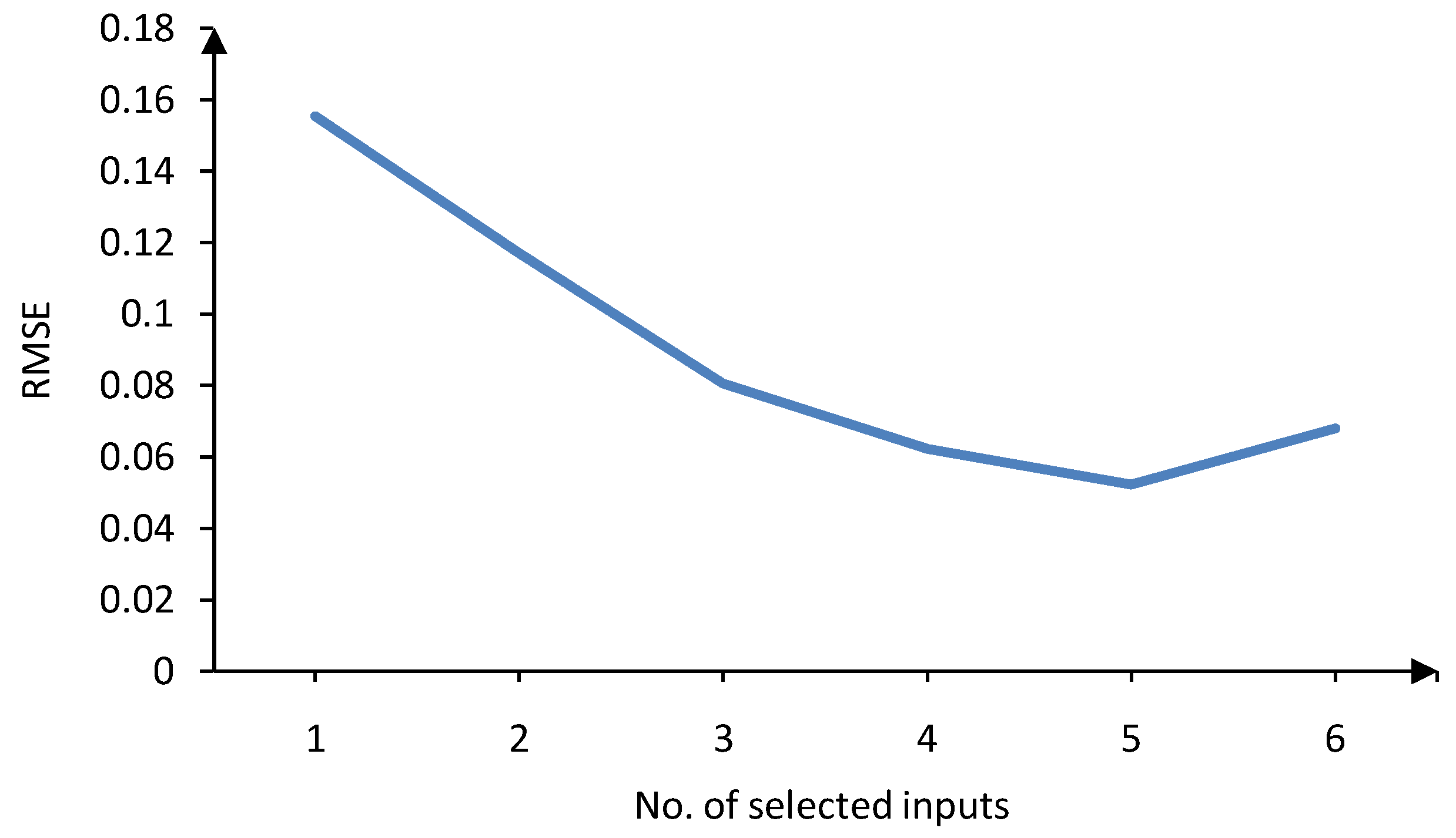
In the model validation steps, at first, only the input with the highest rank is fed to the model. The model is trained with this input and then the validation data are applied to the model and validation error is calculated. Then the input with the second rank is added to the inputs of the mode. Again the model is trained and then the validation error is computed. The process of adding high ranked inputs carries on until no improvement happens in the validation error. The proper number of inputs is decided upon based on the lowest validation error. 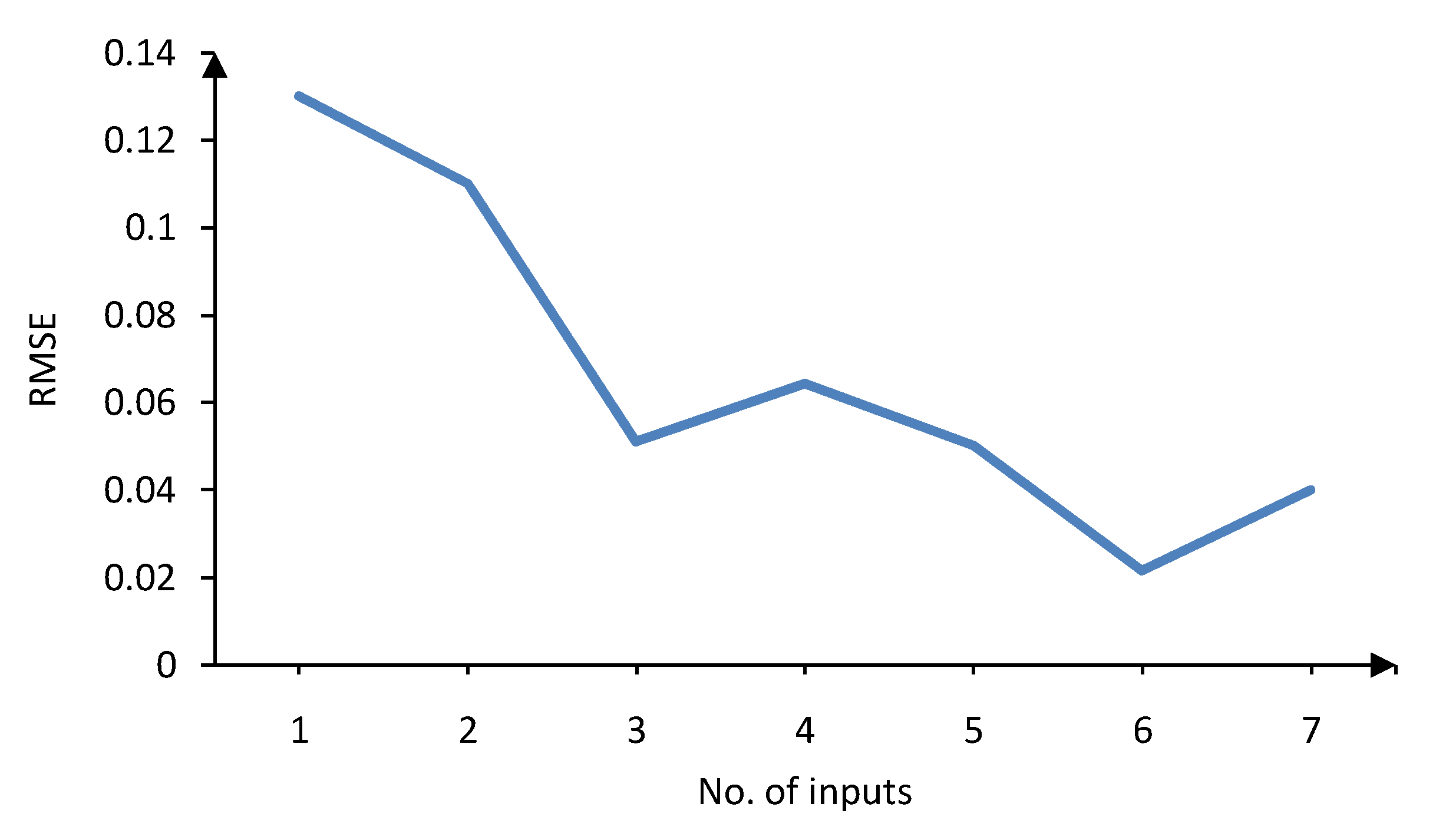The procedure of selecting number of inputs based on the validation error is carried out for both trend (LLNF_τ) and cyclic (LLNF_c) models. The validation errors for trend and cyclic models of the first case study (gasoline demand forecasting) are shown in Figure 5 and Figure 6, respectively. Obviously, six inputs results in the lowest validation error for LLNF_τ model, while five inputs lead to the best validation error for LLNF_c model. These inputs will be used to construct the structure of the forecast model. For further analysis, the selected inputs for both LLNF_τ and LLNF_c of the first case study are presented in Table 3 and Table 4, respectively. The normalized mutual information between each selected input and the output is also presented in these tables. The normalization was performed with respect the input with maximum MI with the output. It’s worth noting that, in addition to the first three past lags of the gasoline demand, the exogenous variables are also assigned to the trend model, LLNF_τ, while only the past time lags of the gasoline demand historical are selected as the inputs of the cyclic model, LLNF_c. This is due to the fact that the trend component represents long-term changes of the demand and therefore is more correlated to the econometric variable such as population and GDP. In Table 3, $d{t}_{h-1}$, $p_{h-1}$, $p{r}_{h-1}$, $GD{P}_{h-1}$ stand for gasoline demand trend component, population, gasoline price and GDP at month $h-1$, used for forecasting the trend of gasoline demand at month h.

Figure 5. Validation error versus number of inputs for LLNF_τ—first case study.

Figure 5. Validation error versus number of inputs for LLNF_τ—first case study.

Figure 6. Validation error versus number of inputs for LLNF_c—first case study.

Figure 6. Validation error versus number of inputs for LLNF_c—first case study.

Table 3. Selected input features for the trend model of the gasoline demand.

Rank	Variable	Normalized MI with the Output
1	${dt}_{h-1}$	1
2	${dt}_{h-2}$	0.86
3	$p_{h-1}$	0.75
4	${dt}_{h-3}$	0.71
5	${pr}_{h-1}$	0.69
6	${GDP}_{h-1}$	0.65

Table 3. Selected input features for the trend model of the gasoline demand.

Rank	Variable	Normalized MI with the Output
1	${dt}_{h-1}$	1
2	${dt}_{h-2}$	0.86
3	$p_{h-1}$	0.75
4	${dt}_{h-3}$	0.71
5	${pr}_{h-1}$	0.69
6	${GDP}_{h-1}$	0.65

Table 4. Selected input features for the cyclic model of the gasoline demand.

Rank	Variable	Normalized MI with the Output
1	${dc}_{h-12}$	1
2	${dc}_{h-6}$	0.80
3	${dc}_{h-24}$	0.77
4	${dc}_{h-36}$	0.65
5	${dc}_{h-30}$	0.55

Table 4. Selected input features for the cyclic model of the gasoline demand.

Rank	Variable	Normalized MI with the Output
1	${dc}_{h-12}$	1
2	${dc}_{h-6}$	0.80
3	${dc}_{h-24}$	0.77
4	${dc}_{h-36}$	0.65
5	${dc}_{h-30}$	0.55

On the other hand, the cyclic trend contains the seasonality nature of the demand series. Therefore the past time lags of the 6, 12, 24, 30 and 36, which represent the demand periodicity, provide the highest information about the future values of the cyclic component. In Table 4, the $d{c}_h$ stands for gasoline demand cyclic component at month h.

6.2. Forecasting Gasoline Demand

Monthly U.S. gasoline demand in 2010 is forecasted as the first case study. The forecasted model is trained using data from January 1992 to December 2008 and validated through data from January 2009 to December 2009. The forecasted and actual values of gasoline demand for test data set are depicted in Figure 7. The forecast was obtained using LLNF model with global estimation. Interestingly, the proposed model has effectively followed variations in gasoline demand.

Figure 7. Actual and forecasted gasoline demand for 2010 (HPLLNF + MI).

Figure 7. Actual and forecasted gasoline demand for 2010 (HPLLNF + MI).

For a better insight, the actual and forecasted values and the corresponding APE are summarized in Table 5. The training and test MAPE are presented in Table 6.

Table 5. Actual and forecasted gasoline demand (HPLLNF + MI).

Actual	Forecast	APE %
8.52	8.58	0.76
8.58	8.68	1.18
8.79	8.84	0.54
9.11	8.92	2.1
9.16	9.02	1.53
9.31	9.05	2.79
9.3	9.27	0.33
9.26	9.29	0.3
9.11	8.9	2.29
9.02	8.93	0.99
8.82	8.86	0.48
8.910	8.907	0.03

Table 5. Actual and forecasted gasoline demand (HPLLNF + MI).

Actual	Forecast	APE %
8.52	8.58	0.76
8.58	8.68	1.18
8.79	8.84	0.54
9.11	8.92	2.1
9.16	9.02	1.53
9.31	9.05	2.79
9.3	9.27	0.33
9.26	9.29	0.3
9.11	8.9	2.29
9.02	8.93	0.99
8.82	8.86	0.48
8.910	8.907	0.03

Table 6. Train and test MAPE—gasoline demand forecasting.

	Training MAPE %	Test MAPE %
HPLLNF (global) + MI	1.05	1.11
HPLLNF (local) + MI	1.08	1.16
LLNF (global) + MI	1.23	1.54

Table 6. Train and test MAPE—gasoline demand forecasting.

	Training MAPE %	Test MAPE %
HPLLNF (global) + MI	1.05	1.11
HPLLNF (local) + MI	1.08	1.16
LLNF (global) + MI	1.23	1.54

Based on these results, the model composed of the HP filter, MI-based input selection and LLNF model with global estimation has the best performance with training MAPE of 1.05% and test MAPE of 1.11%. It must be noted that, in Table 6 we indicated the LLNF mode with global least square estimation as LLNF (global) and the LLNF model with local least square estimation as LLNF (local). Combination of the LLNF model and the HP filter is also referred to as HPLLNF model. Influence of the HP filter on forecasting accuracy can also be analyzed using this table. The test MAPE has been reduced from 1.54% to 1.11% by employing the HP filter. The model performance in the training phase has also been improved due to the HP filter.

6.3. Forecasting Crude Oil Demand

The second case study focuses on crude oil demand forecasting. The input variables and range of required data for training, validating and testing the forecast model have been summarized in Table 1 and Table 2. Similar to previous case study, after extracting the trend and cyclic components of the training and validation data, the LLNF_τ and LLNF_c models are trained and then appropriate number of inputs is determined by applying validation data.

Table 7. Actual and forecasted crude oil demand (HPLLNF (global) + MI).

Actual	Forecast	APE %
19.04	19.44	2.1
18.82	19.21	2.08
18.72	18.79	0.37
18.67	19.05	2.02
18.21	18.73	2.87
18.83	19.06	1.21
18.63	18.97	1.85
18.95	18.96	0.06
18.59	18.16	2.3
18.8	18.85	0.26
18.75	18.69	0.33
19.24	18.78	2.39

Table 7. Actual and forecasted crude oil demand (HPLLNF (global) + MI).

Actual	Forecast	APE %
19.04	19.44	2.1
18.82	19.21	2.08
18.72	18.79	0.37
18.67	19.05	2.02
18.21	18.73	2.87
18.83	19.06	1.21
18.63	18.97	1.85
18.95	18.96	0.06
18.59	18.16	2.3
18.8	18.85	0.26
18.75	18.69	0.33
19.24	18.78	2.39

Figure 8 illustrates the forecasted values of the crude oil demand in 2009 as well as the actual demand. Although the test series exhibits many fluctuations and changes during 2009, but the proposed HPLLNF (global) + MI forecast model has captured the dynamics of the demand series and acceptable forecasts have been provided. The numerical values of actual and forecasted crude oil demand are also given in Table 7. Based on the results presented in Table 5, the APE ranges from 0.06% to 2.87%.

Figure 8. Actual and forecasted crude oil demand for 2009 (HPLLNF (global) + MI).

Figure 8. Actual and forecasted crude oil demand for 2009 (HPLLNF (global) + MI).

Besides, a comparison between different models is carried out as shown by Table 8. The comparison result confirms that the HPLLNF (global) + MI model has the best performance in terms of training and test, while the model without HP filtering, i.e., LLNF (global) + MI has the worst accuracy.

Table 8. Train and test MAPE—crude oil demand forecasting.

	Training MAPE %	Test MAPE %
HPLLNF (global) + MI	1.3	1.48
HPLLNF (local) + MI	1.38	1.64
LLNF (global) + MI	1.55	1.80

Table 8. Train and test MAPE—crude oil demand forecasting.

	Training MAPE %	Test MAPE %
HPLLNF (global) + MI	1.3	1.48
HPLLNF (local) + MI	1.38	1.64
LLNF (global) + MI	1.55	1.80

6.4. Forecasting Natural Gas Demand

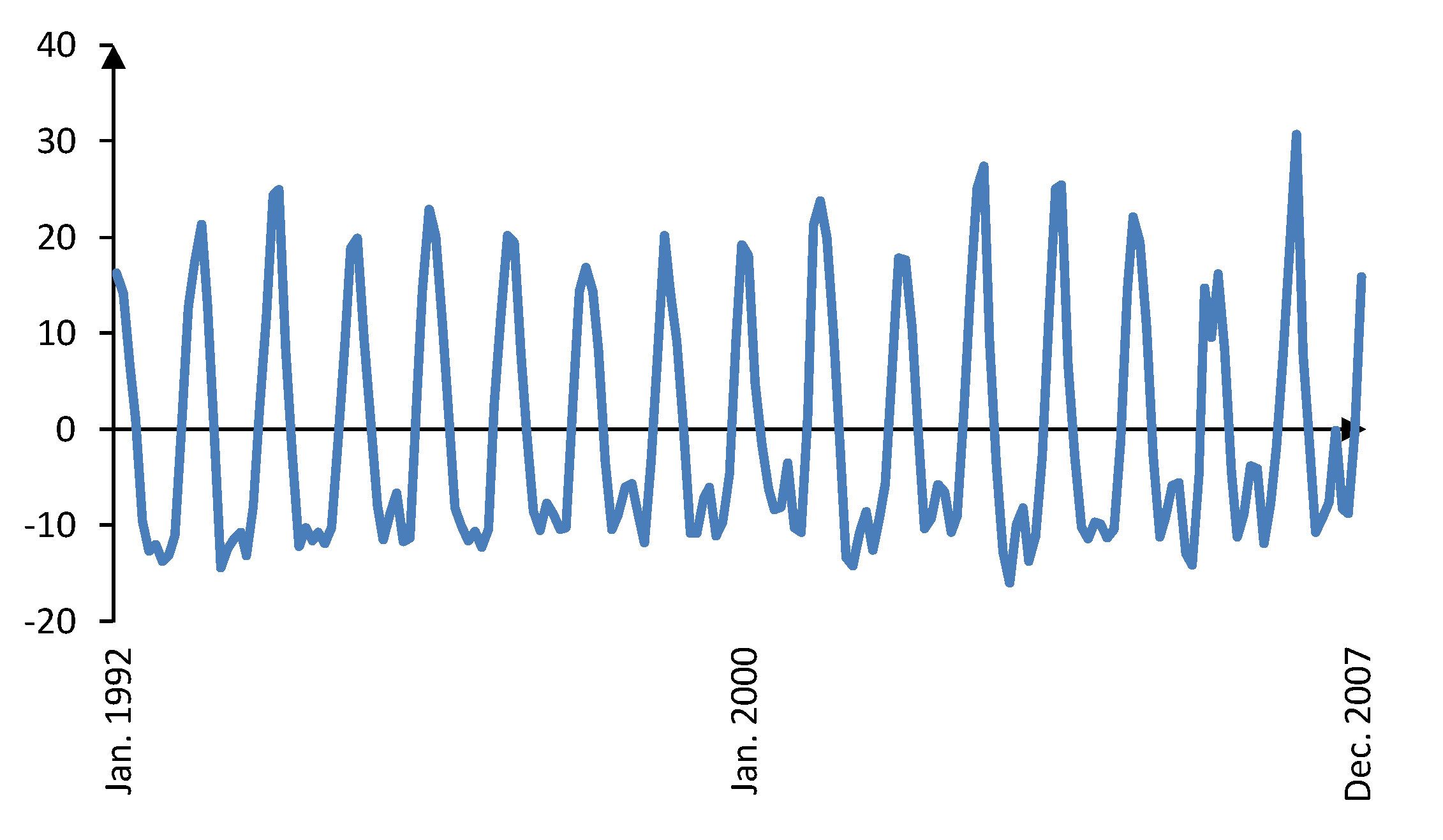
The U.S. natural gas demand forecasting for 2008 is considered as our last case study. Figure 9 shows the original and trend component of the natural gas demand from January 1992 to December 2007. Clearly the trend component contains very long-term variations of the natural gas demand. The corresponding cyclic component is depicted in Figure 10, exhibiting short term and almost seasonal variations. As shown in Table 1, an additional exogenous input variable, i.e., average heating degree-days, has been considered for natural gas demand prediction. This variable reflects the demand for energy needed to heat a home or business and is computed relative to a base temperature.

Figure 9. Original and trend component of the natural gas demand from January 1992 to December 2007.

Figure 9. Original and trend component of the natural gas demand from January 1992 to December 2007.

Figure 10. Natural gas demand cyclic component from January 1992 to December 2007.

Figure 10. Natural gas demand cyclic component from January 1992 to December 2007.

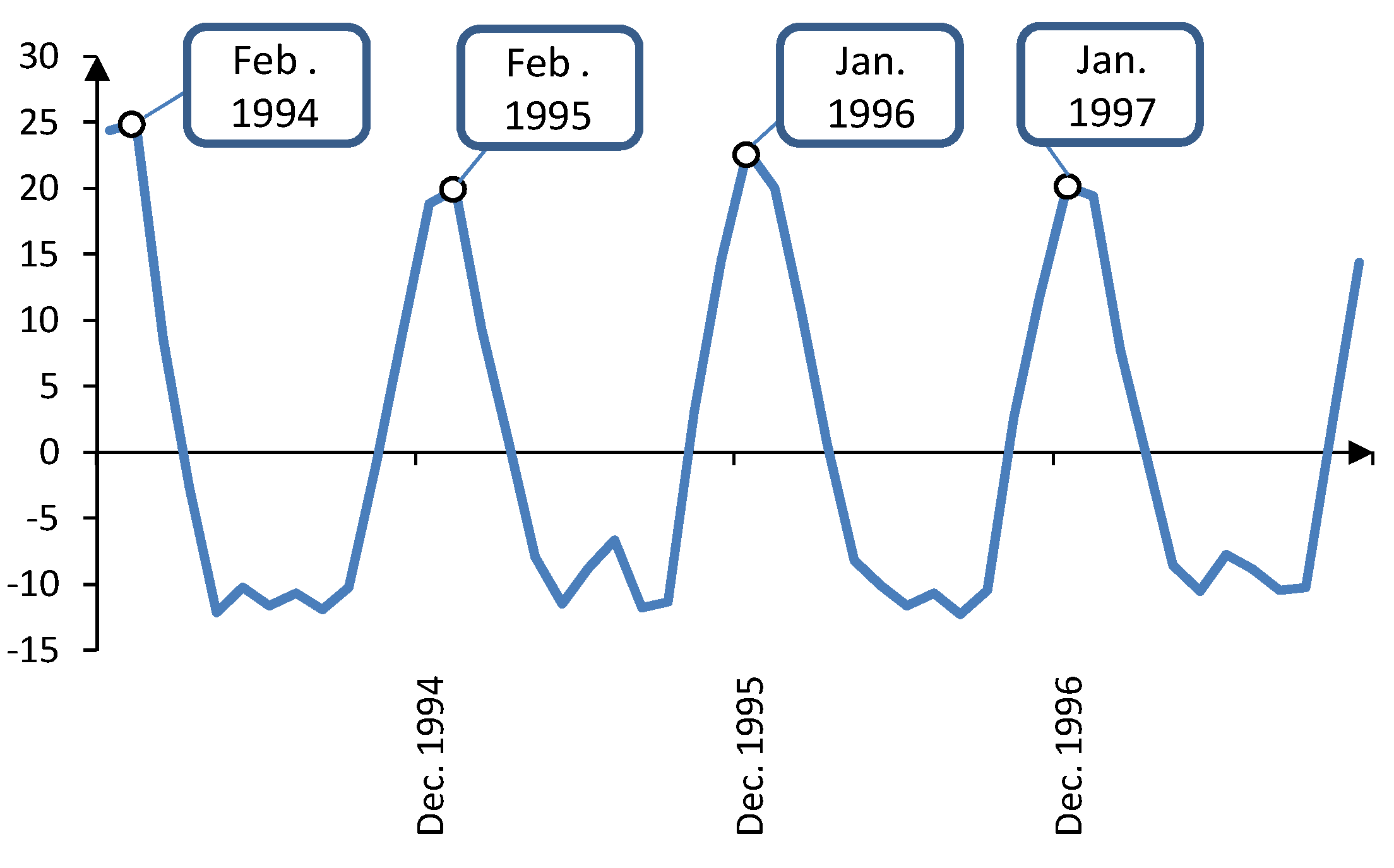
Obviously, the natural gas is consumed during cold months for heating purposes, hence justification of using this variable. Analysis of the cyclic component obtained by the HP filter also supports this discussion. Figure 11 focuses on the the cyclic series from January 1994 to December 1997. It is clear that there are four peaks in the cyclic series within this period, each corresponding to a cold month in the year. 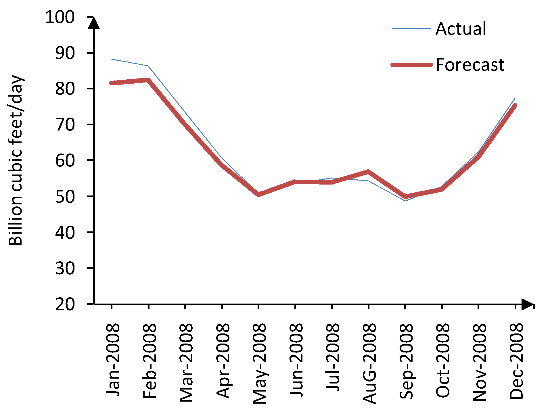The actual and predicted values for natural gas demand in 2008 are shown in Figure 12, demonstrating the noteworthy accuracy of the proposed HPLLNF (global) + MI in long-term natural gas demand forecasting.

Figure 11. Natural gas demand cyclic component from January 1994 to December 1997.

Figure 11. Natural gas demand cyclic component from January 1994 to December 1997.

Figure 12. Actual and forecasted natural gas demand for 2008 (HPLLNF (global) + MI).

Figure 12. Actual and forecasted natural gas demand for 2008 (HPLLNF (global) + MI).

It must be noted that such accurate 12-step ahead prediction have been achieved through HP filter decomposition, efficient input selection by MI, and distinguished modeling capabilities of the LLNF network. The numerical results and the comparison to other models are provided by Table 9 and Table 10, respectively.

Table 9. Actual and forecasted natural gas demand (HPLLNF (global) + MI).

Actual	Forecast	APE %
88.17	81.48	7.58
86.3	82.37	4.55
73.46	69.99	4.73
60.77	58.79	3.25
50.83	50.48	0.69
53.45	54.02	1.07
55.1	53.91	2.16
54.27	56.88	4.81
48.67	49.94	2.6
52.75	51.87	1.66
62.27	60.97	2.08
77.38	75.23	2.77

Table 9. Actual and forecasted natural gas demand (HPLLNF (global) + MI).

Actual	Forecast	APE %
88.17	81.48	7.58
86.3	82.37	4.55
73.46	69.99	4.73
60.77	58.79	3.25
50.83	50.48	0.69
53.45	54.02	1.07
55.1	53.91	2.16
54.27	56.88	4.81
48.67	49.94	2.6
52.75	51.87	1.66
62.27	60.97	2.08
77.38	75.23	2.77

Table 10. Train and test MAPE—natural gas demand forecasting.

	Training MAPE %	Test MAPE %
HPLLNF (global) + MI	2.95	3.16
HPLLNF (local) + MI	3.24	3.37
LLNF (global) + MI	3.66	4.1

Table 10. Train and test MAPE—natural gas demand forecasting.

	Training MAPE %	Test MAPE %
HPLLNF (global) + MI	2.95	3.16
HPLLNF (local) + MI	3.24	3.37
LLNF (global) + MI	3.66	4.1

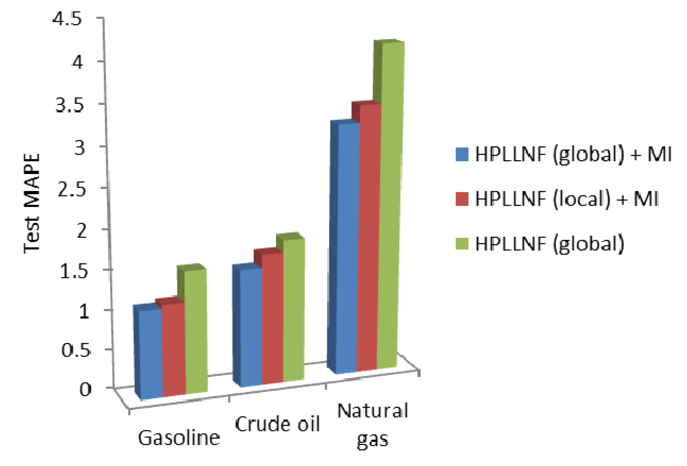
An overall comparison for three case studies is illustrated by Figure 13. In this figure, the values of the test MAPE for three different models are presented. It is clear that in all cases, the HPLLNF model (global) + MI has resulted in the most satisfactory performance.

Figure 13. Comparison of test MAPE in different case studies.

Figure 13. Comparison of test MAPE in different case studies.

7. Conclusions

This paper has proposed a sophisticated long-term energy demand forecasting approach based on the HP filter, MI-based input selection algorithm and LLNF model. Extraction of the trend and cyclic components of the demand series and effective input selection by the MI technique, considerably improved the modeling performance of the LLNF network. Both local and global estimation of rule consequent parameters of the LLNF model were considered and it was demonstrated that the global estimation technique results in higher modeling performance. Due to individual modeling of the trend and cyclic components, selection of different input for each component was made possible and then the overall demand series was modeled more accurately. Implementation of the proposed HPLLNF (global) + MI in three different case studies, demonstrated the ability of the proposed model for long-term energy demand forecasting. The monthly gasoline, crude oil and natural gas demand of the US were forecasted in three different years. The noteworthy forecasting results indicate that the proposed approach can be effectively used in real world energy demand forecasting applications.