Polymer Combustion as a Basis for Hybrid Propulsion: A Comprehensive Review and New Numerical Approaches


Abstract
:1. Introduction
- (1)
- Safety. This is a major attraction. The solid fuel is inert, therefore it can be manufactured, transported and handled safely. In addition, because an intimate mixture of oxidizer and fuel is not possible, it is non-explosive.
- (2)
- Operating issues. Engine throttling and shutdown are significantly simplified by this technology. Throttling is achieved by liquid flow rate modulation, which is considerably simpler in this case compared to a liquid rocket engine where two liquid streams have to be synchronised. Termination is accomplished by cutting of the liquid flow rate. This opens possibility of quick and robust abort procedure.
- (3)
- Choice of fuel. A wide range of easily available solid fuels can be used, giving wider design flexibility compared to liquid or solid motors. Combustion performance of solid fuel is also more reliable since in a hybrid mode it is not sensitive to fuel-grain cracks.
- (4)
- Cost. Operational costs are obviously of great importance. In this regard hybrid systems benefit from simplified manufacturing procedures, due to their inherent safety. Consequently, fabrication (and therefore operation) costs are reduced.
- (1)
- Low regression rate. This is a major obstacle for a wide use of Hybrid Rocket Engines. Essentially non-energetic nature of fuels gives rise to requirement of very high regression rates, in order to achieve required thrust. In practice it leads to necessity to use multiple ports, and other modifications that complicates design.
- (2)
- Combustion efficiency is lower compared to liquid or solid engines, due to non-premixed nature of combustion.
- (3)
- Finally, ignition transient and thrust response to throttling is slower than in solid or liquid motors.

2. Fundamentals of Polymer Combustion
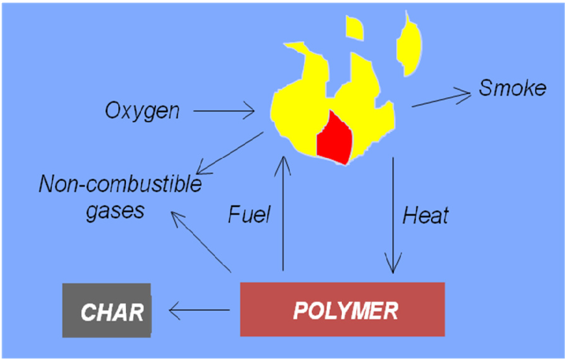
2.1. Flammability Characteristics of Polymeric Materials
- Random chain cleavage followed by chain unzipping is characterized by high monomer yields and a slow decrease in the molecular weight of the polymer, e.g., poly(methyl methacrylate), poly(α-methylstyrene), polystyrene, polytetrafluoroethylene.
- Random chain cleavage followed by further chain scission is characterized by very low monomer yields amongst the degradation products and a rapid drop in molecular weight, e.g., polyethylene, polypropylene, poly(methylacrylate), polychlorotrifluoroethylene.
- An intra-chain chemical reaction followed by cross-linking reaction and formation of a carbonaceous residue, or random chain cleavage. This generates a relatively high yield of volatiles from the intra-chain reaction, but produces little monomer, and produces, no, or only a very slight, reduction in molecular weight during the initial stages of degradation, e.g., poly(vinyl chloride), poly(vinyl alcohol), polyacrylonitrile.

| Polymer | LOI |
|---|---|
| Polypropylene | 18 |
| Poly(butylene terephthalate) | 20 |
| Poly(ethylene terephthalate) | 21 |
| Nylon-6,6 | 24 |
| Nylon-6 | 21 |
| Cotton | 16 |
| Polyester fabric | 21 |
| Wool | 24 |
| Polyacrylonitrile | 18 |
| Polyaramid | 38 |
| Polymer | Peak Heat Release Rate a (kW m−2) |
|---|---|
| Polypropylene | 1095 |
| Poly(butylene terephthalate) | 1313 |
| Isophthalic polyester | 985 |
| Nylon-6,6 | 1313 |
| Nylon-6 | 863 |
| Wool | 307 |
| Acrylic fibres | 346 |
| Polymer Char | Heat Release Capacity (J g−1 K−1) | Total Heat Released (kJ g−1) | Residue (wt.%) |
|---|---|---|---|
| Polypropylene | 1571 | 41.1 | 0 |
| Polyethylene (LDPE) | 1676 | 41.6 | 0 |
| Polystyrene | 927 | 38.8 | 0 |
| Poly(butyleneterephthalate) | 474 | 20.3 | 1.5 |
| Poly(ethyleneterephthalate) | 332 | 15.3 | 5.1 |
| Polymethylmethacrylate | 376–514 | 23.2 | 0 |
| Polyoxomethylene | 169 | 10 | 0 |
| Polyvinylchloride | 138 | 11.3 | 15.3 |
| Polymer | Net Heat of Combustion (kJ g−1) | |
|---|---|---|
| PCFC | Oxygen Bomb | |
| Polyethylene | 44.1 | 43.3 |
| Polystyrene | 40.1 | 39.8 |
| Polycarbonate | 29.1 | 29.8 |
| Poly(butyleneterephthalate) | 26.3 | 26.7 |
| Poly(ethyleneterephthalate) | 23.2 | 21.8 |
| Polymethylmethacrylate | 25.0 | 25.4 |
| Polyoxomethylene | 15.0 | 15.9 |
2.2. Combustion of Some Representative Polymeric Solid Fuels
2.2.1. Polyolefins
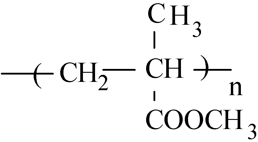
2.2.2. Acrylics
2.2.3. Elastomers
2.3. Enhancement in Degradation and Regression Rates in Hybrid Fuels—Some Suggestions for Future Work
- (a)
- Spectroscopic (NMR and FT-IR) and elemental analyses—high field (500 MHz) solution state 1H- and 13C-NMR for deciphering the microstructures of the polymers (this includes tacticity, composition, monomer sequencing, minor structures including structural defects, etc.). Limited, but complementary, information regarding the structural features of the polymer could also be obtained from the FT-IR spectra and heteroatom elemental analyses.
- (b)
- Chromatographic and related techniques—these are primarily aimed at obtaining the molecular weights and their distributions. For polyolefin based-polymers, optionally melt-flow index measurements could be carried out.
- (c)
- Thermo-gravimetric analyses (TGA)—TGA runs need to be carried out on ca. 10–15 mg of the resin in nitrogen, air and in oxygen atmospheres, say, at 10 °C min−1, and from 30 to 1000 °C. The idea behind these runs is to get the general thermal- and thermo-oxidative degradation profiles of the material (i.e., under different oxidative atmospheres). This could be followed by repeating the runs, in a chosen atmosphere(s), with a view to estimating the Arrhenius parameters, if necessary.
- (d)
- Differential Scanning Calorimetry (DSC)—here, milligrams of samples are heated in sealed aluminium pans, under a nitrogen atmosphere and usually at a heating rate of 10 °C min−1, up to a point where substantial thermal degradation starts. This is a very useful technique that often yields information regarding melting behaviours, glass transition temperatures, etc. that the material might undergo under the heating conditions imposed.
- (e)
- Parallel Plate Rheometry—here again the sample, ideally in the shape of thin films, is heated whilst sandwiched between two heated parallel plates, at the same time a sinusoidal mechanical stress is applied. Generally, this constitute a good method for determining the moduli of elasticity (store and loss), the glass transition temperatures, and more importantly the melt flow behaviour of the resin
- (f)
- Combustion Bomb Calorimeter—this instrumentation is used to determine the heats of combustion (ΔHcomb) of the resin. This parameter is a good indicator of the maximum heat out put on complete oxidation of the polymeric material in question.
- (g)
- Pyrolysis Combustion Flow Calorimetry (PCFC)—this piece of instrumentation, often dubbed as the micro cone calorimeter, produces plots of Heat Release Rates against time, as well as generates parameters like the heat release capacity on milligrams of a material (i.e., the maximum amount of heat released per unit mass per degree of temperature (Jg−1K−1, is a material property that appears to be a good predictor of flammability).
- (h)
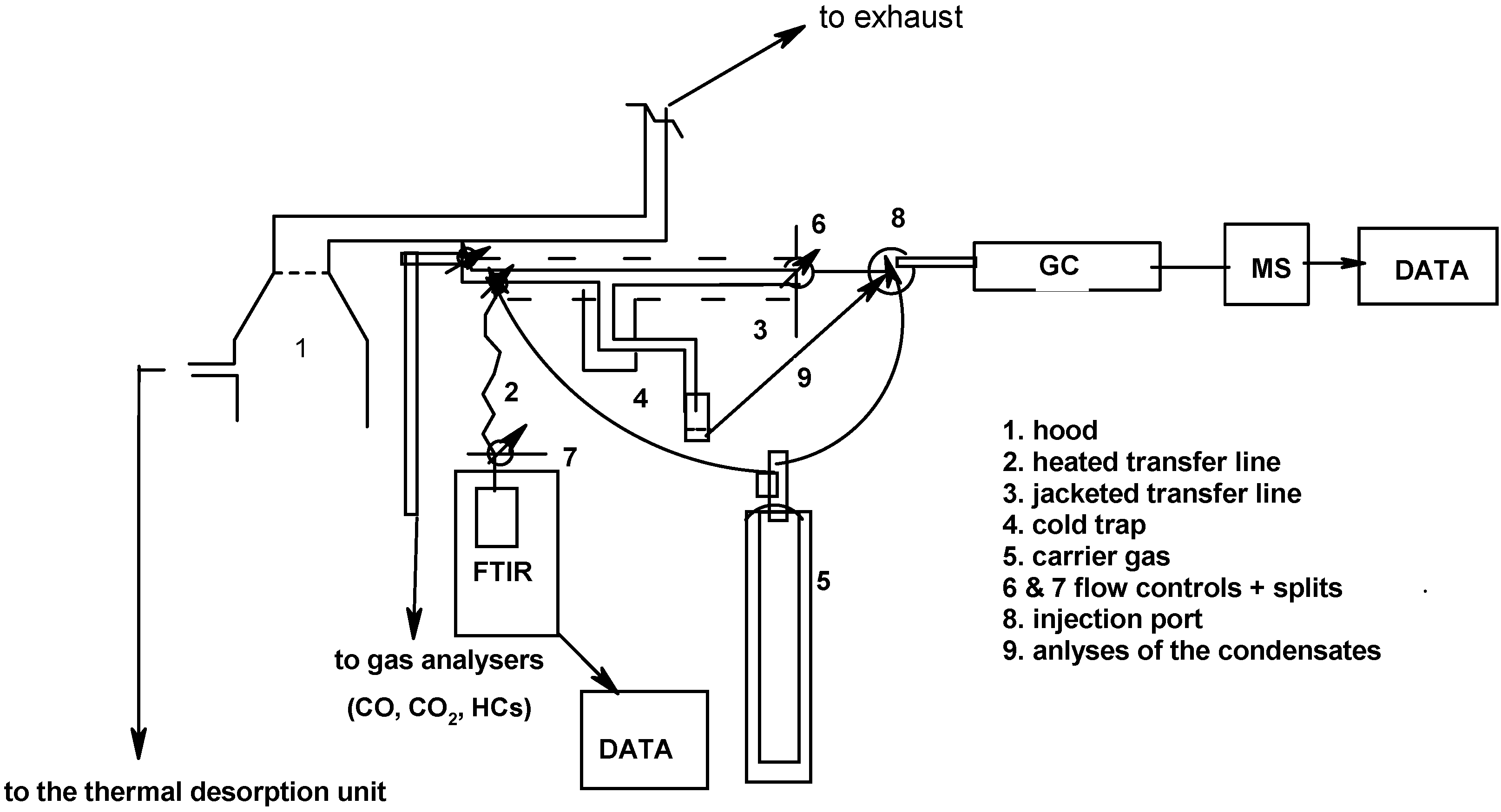
- Hyphenated techniques—attempts to identify the volatiles formed from thermal degradation of the materials could be made by hyphenating the TGA to an FT-IR or to a GC/MS. Such hyphenated technique is also available in a larger scale that, primarily, involves two consecutive tube furnaces in connected in series. Optionally, some of the gaseous-products formed upon degradation, in ambient atmosphere, collected through by using proprietary containers, will be subjected to GC/MS.
3. CFD Modelling Framework for Hybrid Propulsion
3.1. Fuel Regression
- Thermal decomposition
- Thermo-oxidative decomposition
- Decomposition of monomer MMA
- Combustion of pyrolysis products

3.2. Polymer Decomposition Modelling
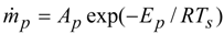
| Ap | pyrolysis pre-exponential factor, kg/(m2 s) | ~8 × 10¹⁷ |
| Ep | pyrolysis activation energy, J/mol | ~2.8 × 10⁵ |
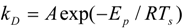
| Polymer | A (s−1) | E (J mol−1) | hD (J kg−1) | hC (J kg−1) |
|---|---|---|---|---|
| PMMA | 8.5 × 10¹² | 1.88 × 10⁵ | 8.7 × 10⁵ | 2.41 × 10⁷ |
| HIPS | 1.2 × 10¹⁶ | 2.47 × 10⁵ | 1.0 × 10⁶ | 3.81 × 10⁷ |
| HDPE | 4.8 × 10²² | 3.49 × 10⁵ | 9.2 × 10⁵ | 4.35 × 10⁷ |
| Ea (kcal/mol) | ln A (s−1) | T (°C) | Ref. | Comments |
|---|---|---|---|---|
| 31 ± 3 a | – | cis-trans Isomerization 200–300 | [3] a | IR, vacuum |
| 15 a | – | Cross-linking and Cyclization 200–300 | [9] | IR, vacuum, first order, vinyl groups |
| 18.8 b | 2.5 | 328–420 | [4] | TGA |
| 27.6 ± 1.6 b | 16.2 | 350–400 | [13] b | TGA |
| 39 | – | 250 | [11] | Hardening data |
| 37.6 c | 25.6 | Chain Scission 450–532 | [15] | pyrolysis-GC, BD formation, first order |
| 40.7 ± 3 | – | N/A | [10] | estimate of 4-vinyl-1 cyclohexene formation |
| 42.1 a | – | 362–434 | [10] | DSC |
| 42.8 | – | – | [16] | Estimate |
| 46 ± 0.6 b | 22.8 | 436–470 | [4] | TGA |
| 51.9 a | 350–425 | [10] | TGA | |
| 60.0 ± 3.5 a | – | N/A | [10] | Estimate of BD formation |
| 60.1 b | 17.1 | 367–407 | [13] | TGA |
| 62 | – | 380–395 | [14] | weight change |
| 62 ± 4 d | – | 410–500 Unspecified Processes | [6] | TGA |
| 24.5–38.5 e | 12.2-20.8 | 350–550 | [7] | TGA |
| 28 e | 12.8 | 400–500 | [18] | TGA, order = 0.6–1 |
| 21.5–31.1 b | 8.9–13.8 | N/A | [19] | TGA |
3.3. Polymer Combustion Modelling
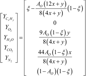
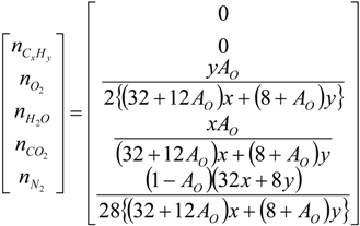
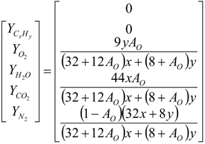
3.3.1. Global Kinetics
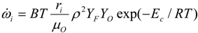
| B | combustion pre-exponential factor, m3 /(s mol K) | ~6.6 × 10⁶ |
| Ec | combustion activation energy, J/mol | ~1.44 × 10⁵ |
3.3.2. Detailed Kinetics
| CH3OH + O2 → CH2OH + HO2 | CHO + O2 → CO + HO2 |
| CH3OH + HO2 → CH2OH + H2O2 | CH2O + HO2 → CHO + H2O2 |
| CH2OH + O2 → CH2O + HO2 | HO2 + O2 → inner products |
| CH2O + O2 → CHO + HO2 |
| HCHO + O2→HO2 + CO | HCO3H → OH + Products |
| HCHO + O2→OH + Products | HO2 + HCHO → H2O2 + HCO |
| (HCOOH or H2 + OO + H2O) | |
| HCHO + OH → H2O + HOO | HO2 + HO2 → H2O2 |
| HOO + M → H + OO + M | H2O2 → HO2 + 1/2 O2 |
| HOO + O2 → HO2 + OO | H2O2 + M → 2OH + M |
| HOO + O2 → HCO3 | HO2 → 1/2 H2O + 3/4 O2 |
| HCO3 + HCHO → HCO3H + HCO |
| C2H2 + M C2H + H + M | CH2 + CH2 C2H4 + H |
| C2H2 + C2H2 C4H2 + H | CH2 + CH2 C2H4 + H2 |
| C2H2 + O2 CHO + CHO | CH2 + CH2 C2H5 + H |
| C2H2 + H C2H + H2 | CH2 + H CH + H2 |
| C2H2 + O CH2 + CO | CH2 + O2 CO2 + H + H |
| C2H2 + O CHCO + H | CH2 + CH2 C2H2 + H + H |
| C2H2 + CH C2H + H2O | C2H6 CH2 + CH2 |
| C2H2 + CH CH2CO + H | C2H6 + H C2H5 + H2 |
| C2H2 + CH C2H2 | C2H6 + CH C2H5 + H2 |
| C2H2 + CH2 C2H4 | C2H6 + CH2 CH4 + C2H5 |
| C2H2 + CH2 C2H + CH4 | C2H5 C2H4 + H |
| C2H2 + C2H C4H2 + H | C2H4 + M C2H2 + H2 + M |
| C2H2 + C2H2 C4H4 + H | C2H4 + H C2H2 + H2 |
| C2H + O2 CO + CO + H | C2H4 + O CH2 + CHO |
| CH2CO + M CO + CH2 + M | C2H4+ CH C2H2 + H2O |
| CH2CO + H CHCO + H2 | C2H2 + M C2H2 + H + M |
| CH2CO + H CH2 + CO | C2H2 + H C2H2 + H2 |
| CH2CO + O CH2 + CO2 | C2H2 + O CH2CO + H |
| CH2CO + O CH2O + CO | C2H2 + O2 C2H2 + HO2 |
| CH2CO + CH CH2O + CHO | C2H2 + O2 CH2O + CO + H |
| CH2CO + CH CH2CH + CO | C2H2 + CH2 C2H2 + CH4 |
| CH2CO + CH2 C2H4 + CO | C2H4 + M C2H2 + H + M |
| CH2CO+ CH2 CHCO + CH3 | C2H4 + H C2H2 + H2 |
| CH2CO+ CH2 C2H5 + CO | C2H4 + H C2H2 + CH2 |
| CH2CO+ CH2 CHCO + CH4 | C2H4 + CH2 C2H2 + CH4 |
| CHCO + O CO + CO + H | C4H4 CH2CO + CH2 |
| CHCO + OH CO + CO + H2 | C4H4 C4H2+ H |
| CHCO + O2 CO + CO + CH | C4H4 C2H2 + C2H2 |
| CHCO + H CH2+ CO | C4H4 C4H2 + H2 |
| CHCO + CH2 C2H2 + CO | C4H4 + H C4H2 + H2 |
| CHCO + CH2 C2H4 + CO | C4H4 + H C4H2 + H2 |
| CHCO + CHCO CO + CO + C2H2 | C4H2 + M C4H2 + H + M |
| CH2O + H CHO + H2 | C4H2 + H C4H2 + H2 |
| CH2O + CH CHO + H2O | C4H2 + C2H C2H2 + H |
| CHO + M CO + H+ M | O2+ H CH + O |
| CHO + H H2+ CO | H2+ O CH + H |
| CHO + O2 HO2+ CO | H2O + H CH + H2 |
| CH2O + M CH2O + H+ M | H + O2+ M HO2 + M |
| CH2OH + M CH2O + H+ M | HO2 + H H2 + O2 |
| CO + CH CO2 + H | HO2 + H CH + OH |
| CH4+ M CH2 + H + M | N2O + M N2 + O + M |
| CH4+ H CH2 + H2 | N2O + O N2 + O2 |
| CH4+ O CH2 + OH | N2O + O NO + NO |
| CH4+ CH CH2+ H2O | N2O + H N2+ OH |
| CH4+ CH2 CH2 + CH2 | N2O + CH2 CH2O + N2 |
| CH2+ H CH2 + H2 | N2O + CH2 CH2O + N2 |
| CH2+ O CH2O + H | N2O + C2H2 CH2CHO + N2 |
| CH2+ CH CH2O + H2 | N2O + CO CO2 + N2 |
| CH2+ CH CH2CH + H | N2O + CHO CO2 + H + N2 |
| CH2+ O2 CH2O + O | N2O + CHCO CO + CHO + N2 |
| CH2+ HO2 CH2O + CH | N2O + C2H2 CHCO + H+ N2 |
| Product | Content v/v % | |||||||
|---|---|---|---|---|---|---|---|---|
| PMMA (air) | MMA (Ar) | MMA (air) | ||||||
| 300 °C | 500 °C | 300 °C | 400 °C | 500 °C | 300 °C | 400 °C | 500 °C | |
| MMA | 95.5 | 78.9 | 92.7 | 83.8 | 74.2 | 91.6 | 79.8 | 68.2 |
| CH4 | 0.8 | 1.3 | 0.6 | 1.5 | 2.6 | 0.5 | 1.2 | 2.2 |
| CH2-CHCH3 | 1.7 | 1.1 | 2.3 | 3.4 | 1.0 | 1.4 | 2.9 | |
| CH2-C(CH3)2 | 1.9 | 1.0 | 2.4 | 3.8 | 1.2 | 1.8 | 3.0 | |
| CH3OH | 1.8 | 3.2 | 1.6 | 3.6 | 5.8 | 1.5 | 2.9 | 4.9 |
| HCHO | 0.3 | 0.5 | 0.8 | |||||
| CH3COCH3 | 0.6 | 0.2 | 0.5 | 1.0 | 0.8 | 1.3 | 1.6 | |
| CH3COCOOCH3 | 0.8 | 1.2 | 2.0 | |||||
| CO2 | 0.8 | 6.0 | 0.9 | 2.0 | 3.3 | 1.4 | 5.2 | 8.0 |
| CO | 0.2 | 0.3 | 1.4 | 3.3 | 5.4 | 1.1 | 0.4 | 0.3 |
| H2O | 0.4 | 4.5 | 0.6 | 3.8 | 5.6 | |||
3.3.3. Fourier Transform Infrared Spectroscopy (FTIR) and Gas Chromatography/Mass Spectrometry (GC/MS)
3.4. Crucial Submodels and Implementation
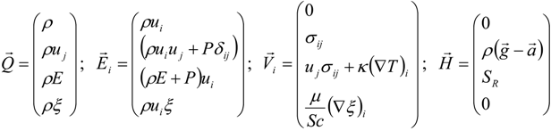
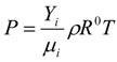
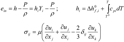
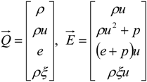
3.4.1. Flow Model

3.4.2. Combustion Modeling
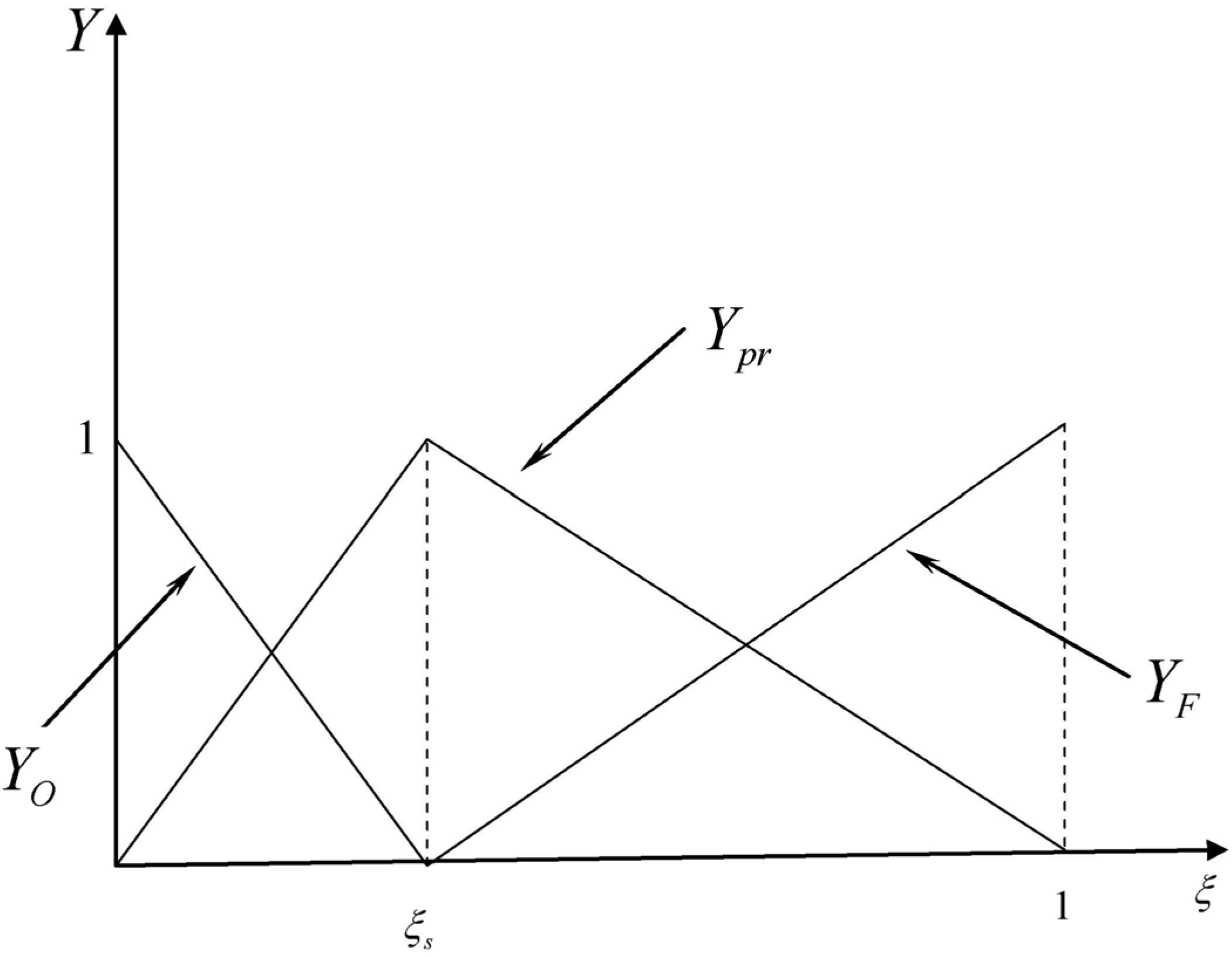
3.4.2.1. Fast Chemistry Approach


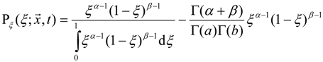
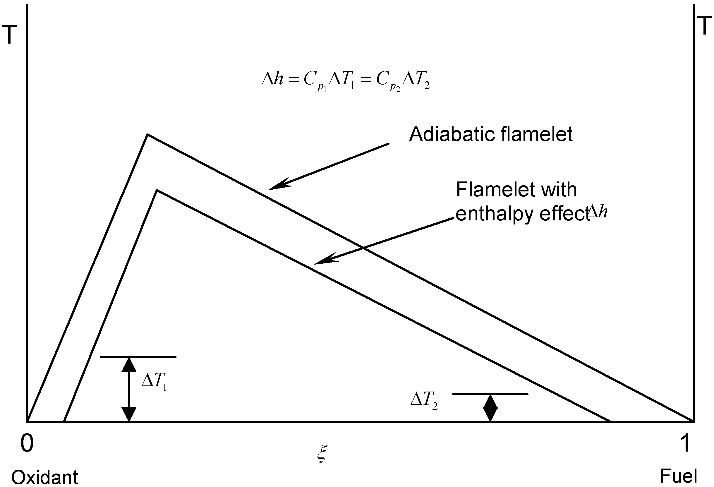
3.4.2.2. Flamelet Approach

3.4.3. Fuel Regression Model


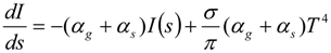
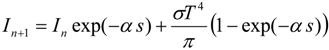
3.4.4. Radiation Heat Transfer
3.4.4.1. Radiation Correction


3.4.4.2. Comprehensive Radiation Modeling


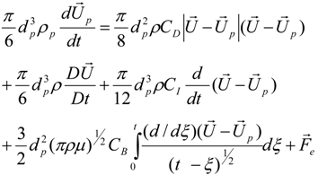
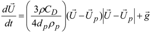
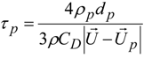
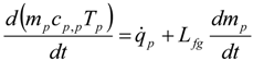
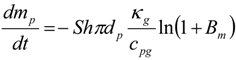
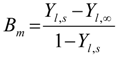
3.4.5. Injector Spray Model


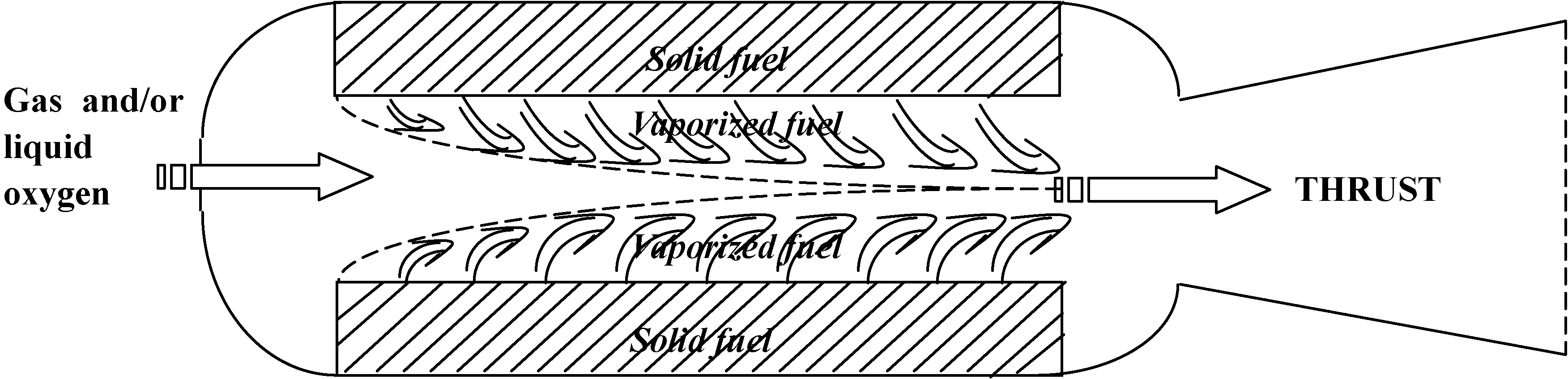
4. Preliminary Simulations

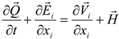
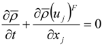
4.1. Implicit Large Eddy Simulation

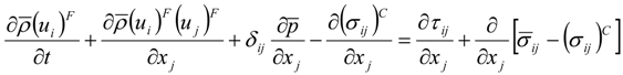
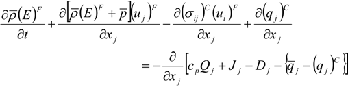
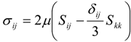
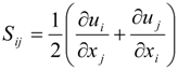
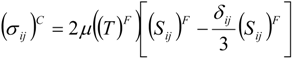 which depends on the computable rate-of-strain tensor
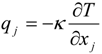
 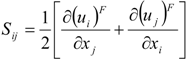 , and the computable heat flux
 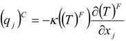 .
.


4.2. Combustion Model


4.3. Numerical Methodology

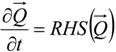
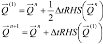
4.3.1. Time Integration
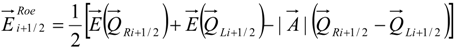
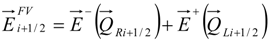
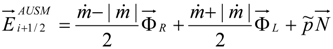
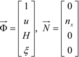
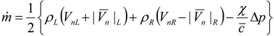
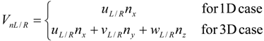
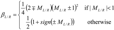
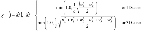
4.3.2. Numerical Flux Function


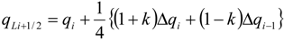
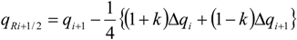
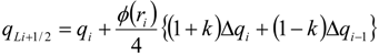
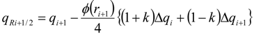
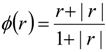
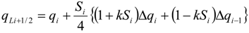
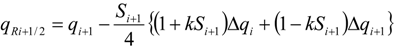
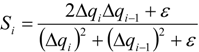
4.3.3. High Order Interpolation Method
| k | Scheme |
|---|---|
| −1 | second-order upwind |
| 0 | second-order |
| 1/3 | third-order upwind |
| 1/2 | QUICK (second-order upwind) |
| 1 | second-order central |

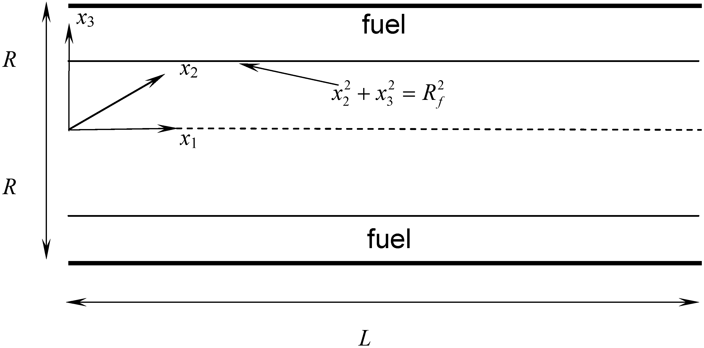
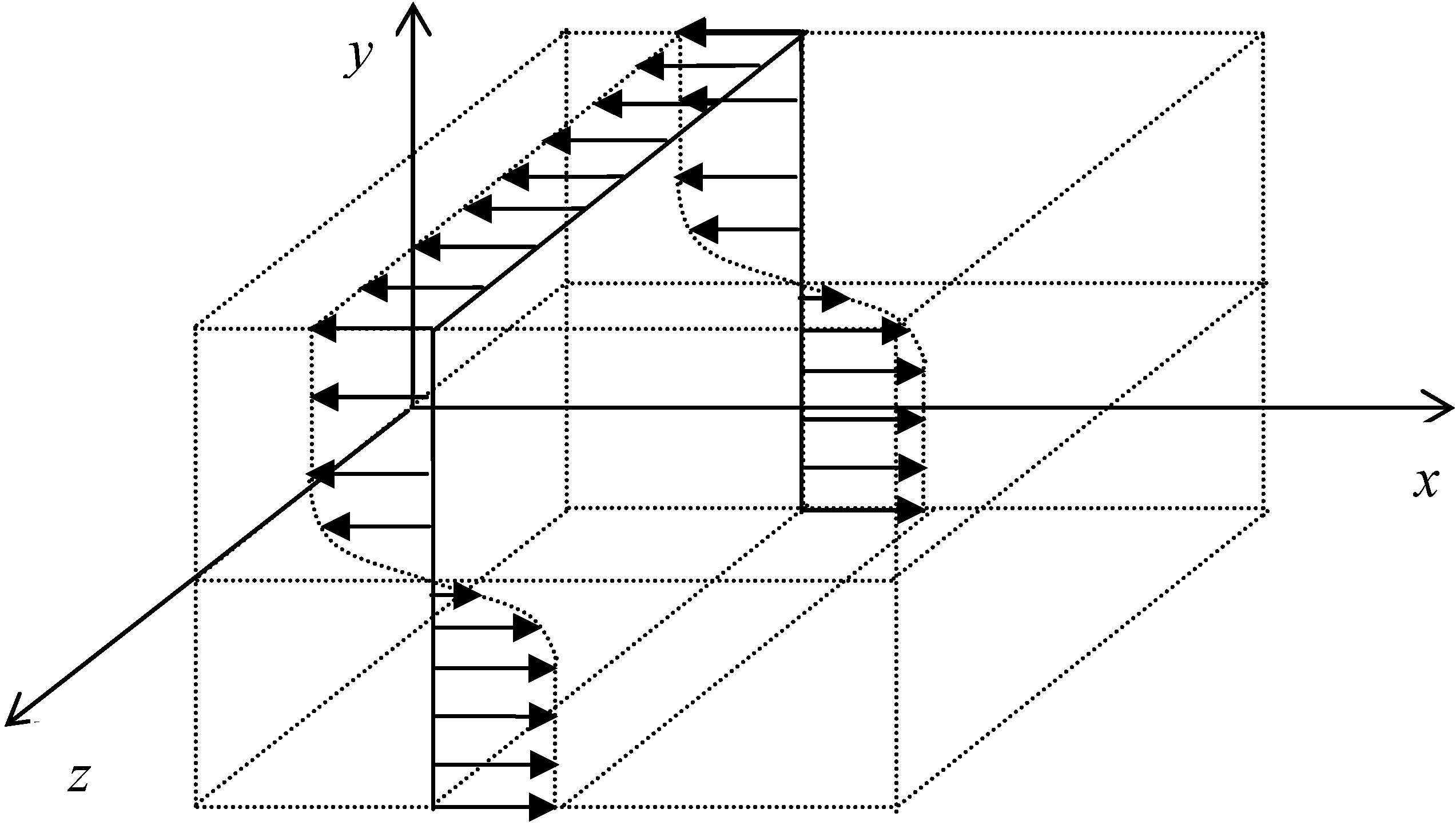
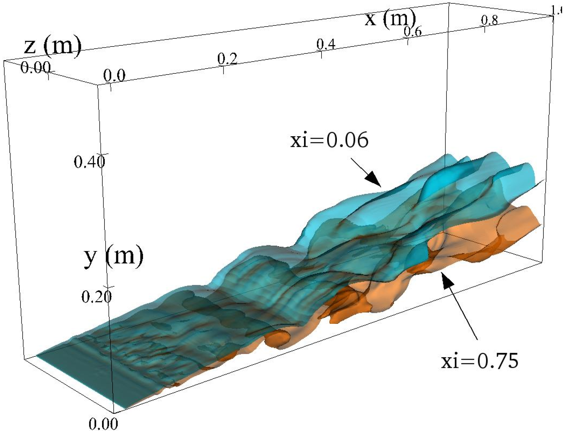
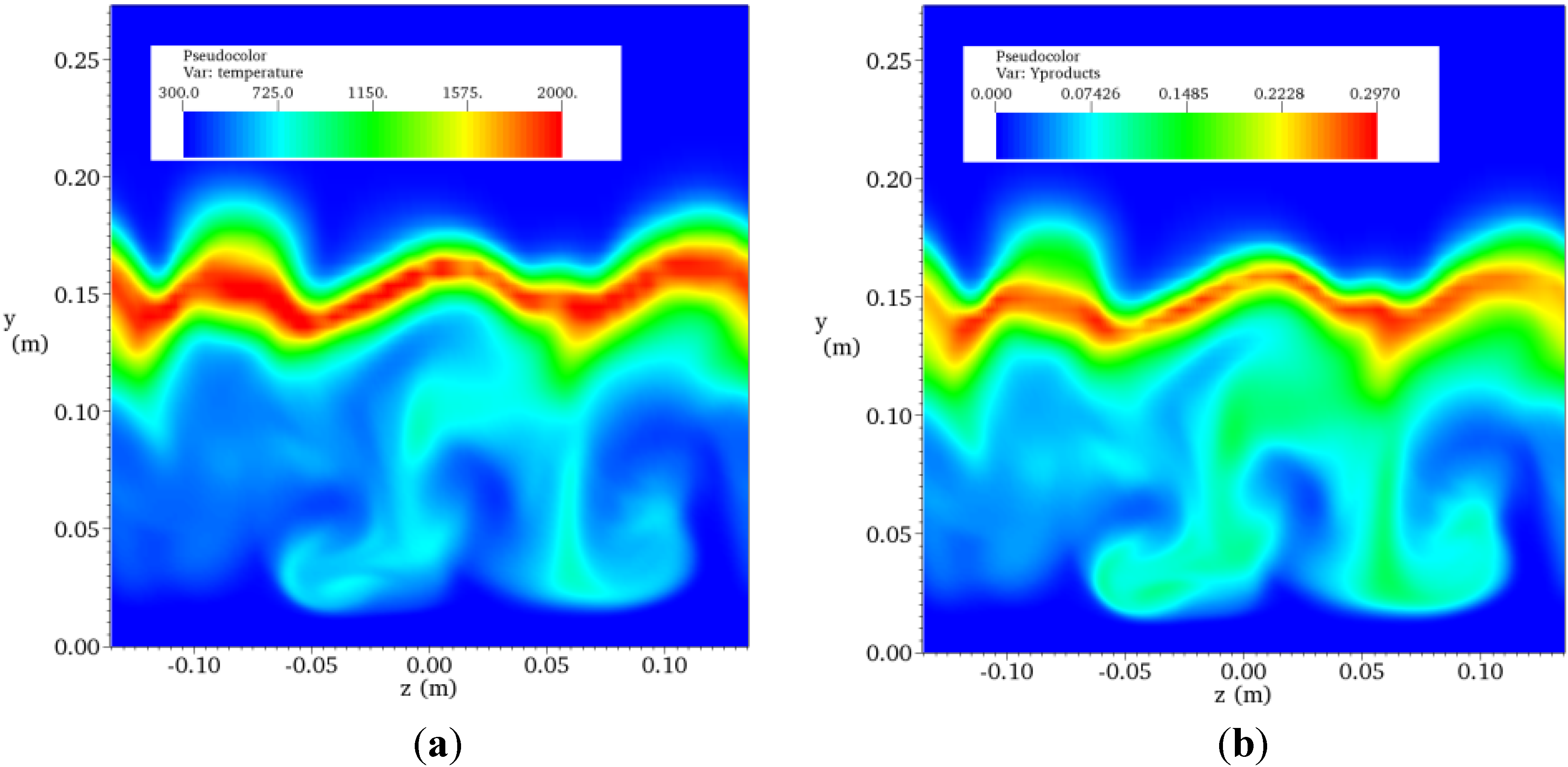
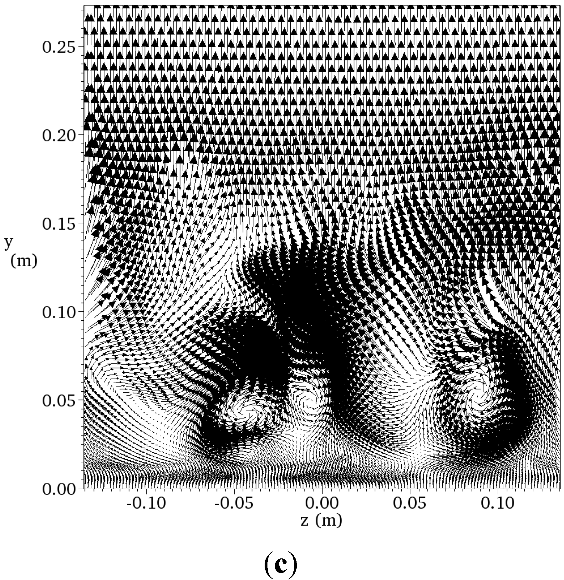
4.4. Non-Premixed Flame in Three-Dimensional Flowfield
4.4.1. Brief Description for Computation

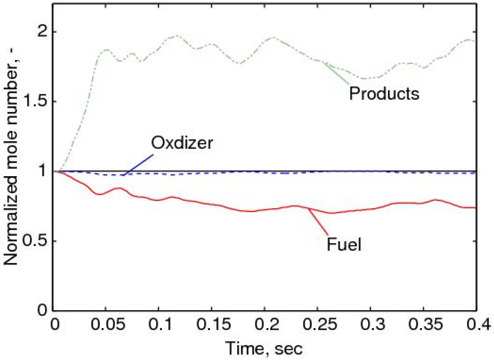
4.4.2. Results and Discussions


| Resolution | Grid Points | CPU Numbers | Total CPU Times per 104 Time Steps |
|---|---|---|---|
| Fine | 253 × 182 × 151 | 16 | 10.64 h |
| Coarse | 201 × 151 × 101 | 8 | 5.34 h |


5. Conclusions
Acknowledgements
Nomenclature
 | flux Jacobian matrix,  |
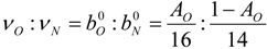
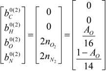
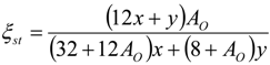
| AO | mass fraction of element O in the air (0 ≤ AO ≤ 1) |
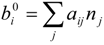
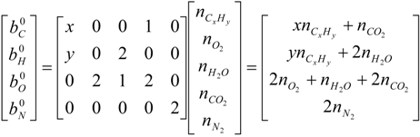
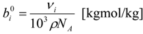
 | mole number for i-th element per unit mass of mixture gas [kgmol/kg] |
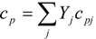
| cp, cp(T) | specific heat at constant pressure [J/(kg K)] |
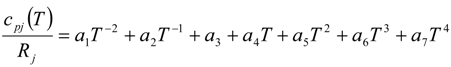
| cpj(T) | specific heat at constant pressure for j-th chemical species [J/(kg K)] |
| cv(T) | specific heat at constant volume [J/(kg K)] |
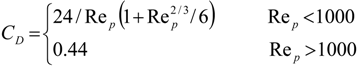
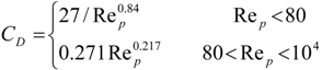
| CD | drag coefficient |
| cf | friction coefficients |
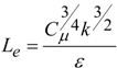
| Cμ | k-ε model constant |
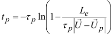
| d | diameter [m] |
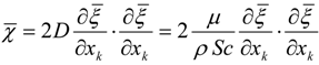
| D | diffusion coefficient [m2/s] |
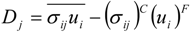
| Dj | subgrid scale (SGS) viscous diffusion |
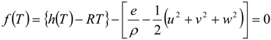
| e | total energy per unit volume [J/m3] |
| ein | internal energy [J/kg] |
| E | total energy per unit mass [J/kg] |
 | inviscid flux vector |
 | numerical flux vector at the cell interface |
 | obtained flux by flux vector splitting methods |
| G | kernel of filter |
| h | enthalpy per unit mass [J/kg] |
| hC | convective heat transfer coefficient [W/ m2 K] |
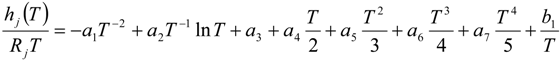
| hj(T) | internal enthalpy per unit mass j-th chemical species [J/kg] |
| H | total enthalpy per unit mass [J/kg] |
| I | total radiation intensity [W/ m2/sr] |
| Jj | subgrid scale (SGS) turbulent diffusion |
| k | parameter deciding the spatial accuracy of MUSCL;turbulent kinetic energy [m2/s2] |
| Lfg | latent heat of liquid evaporation [kJ/kg] |
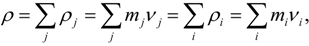
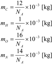
| mi | mass of i-th element [kg] |
| mj | mass of j-th molecule [kg] |
 | mass flux [kg/(m2 s)] |
 | pyrolysis rate [kg/(m2 s)] |
| Nu | Nusselt number |
| n | mole number for mixture gas per unit mass of mixture gas [kgmol/kg] |
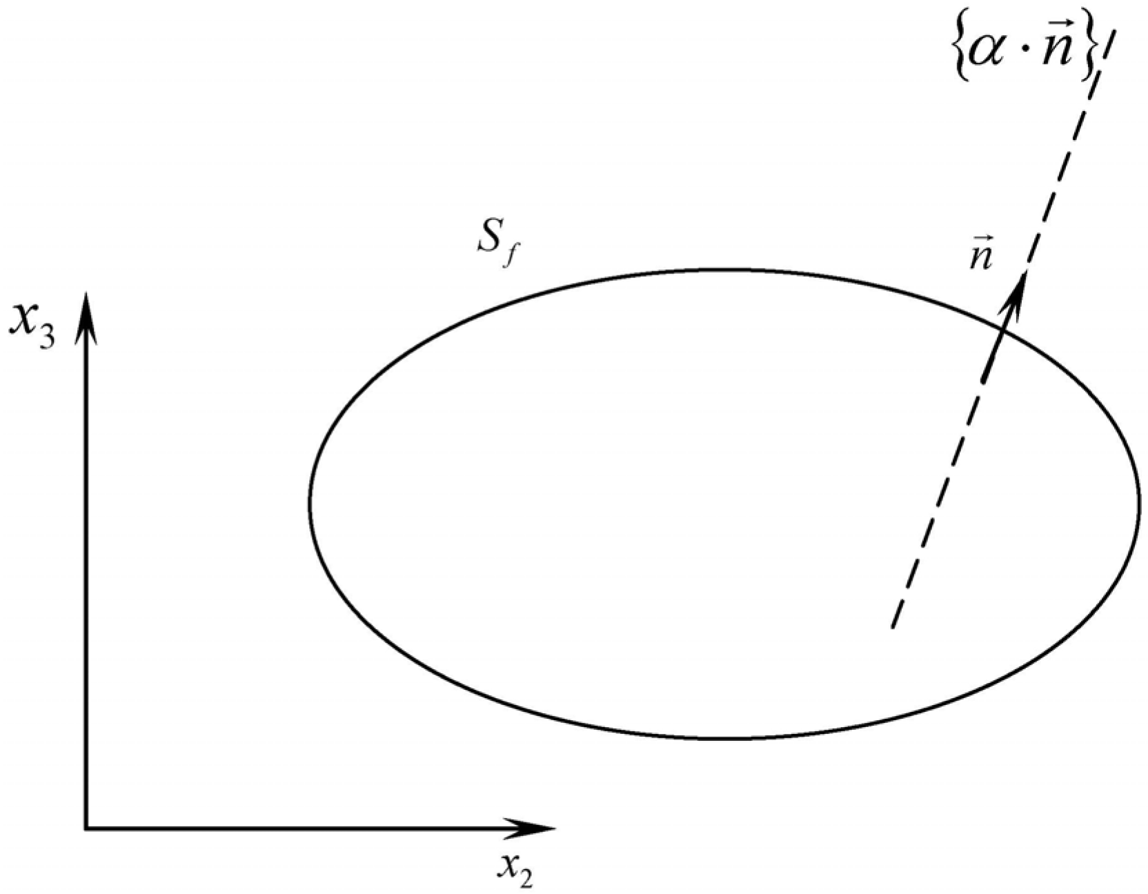
 | inner normal to fuel surface |
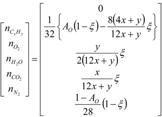
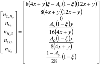
| nj | mole number for j-th species per unit mass of mixture gas [kgmol/kg] |
| nx, ny, nz | Cartesian components of a normal vector from the left to the right at cell interface |
| nj | component of normal vector to ∂Ω |
| p, P | pressure [Pa] |
 | corrected pressure term [Pa] |
| Pr | Pandtl number |
| qj | heat flux [J/(m2 s)] |
| (qj)C | computed heat flux [J/(m2 s)] |
| qi | primitive variables |
 | radiative flux [W/m2] |
 | droplet heating rate [W] |
| Δqi | = qi+1 − qi |
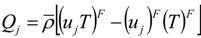
| Qj | subgrid scale (SGS) temperature flux |
 | conservation vector |
| R | gas constant for mixture gas [J/(kg K)] |
| Rj | gas constant for j-th chemical species [J/(kg K)] |
| Re | Reynolds number |
| r | stoichiometric requirement |
| ri | = ∆qi−1/qi stoichiometric requirement for species i with respect to fuel |
| Rf | fuel surface |
| Sc | Schmidt number |
| SR | radiation source term [W/m3] |
| St, St0 | Stanton numbers |
| Sij | rate-of-strain tensor |
| Si | slope limiter function by Van Leer |
| T | temperature [K] |
| Tf | solid fuel temperature [K] |
| T0 | reference temperature |
| ui | Cartesian velocity components corresponding to (u, v, w) [m/s] |
 | cartesian coordinate [m] |
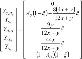
| Y | mass fraction |
| Δx, Δy, Δz | cut-off scale in each direction of the Cartesian coordinate |
 | enthalpy of formation [J/kg] |
| ΔHsg | Heat of pyrolysis [kJ/kg] |
| ε | internal energy [J/kg] energy dissipation rate [m2/s3] |
| ϕ | primitive variables |
| ϕ(ri) | flux limiter |
| γ | ratio of specific heats |
| κ | thermal conductivity (gas) [J/(m s K)] |
| κs | solid thermal conductivity (gas) [J/(m s K)] |
| μ | coefficient of molecular viscosity [kg/(m s)] |
| μi | molecular weight [kg/mol] |
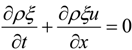
| ρ | density [kg/m3] |
| ∜ | set of real numbers |
| υi | number density for i-th element [m−3] |
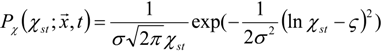
| χ | scalar dissipation rate [s−1] |
| σij | shear-stress tensor |
| (σij)C | computed shear-stress tensor |
| τij | subgrid scale (SGS) scale stress |
| Ω | a control volume |
| ∂Ω | a surface of the control volume |
| ωi | species production rate [kg/m3/s] |
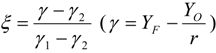
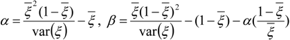
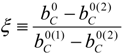
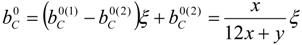
| ξ | mixture fraction of fuel |
| ξst | mixture fraction of fuel at the stoichiometric condition |
Constant values
| NA | Avogadro constant = 6.02214179 [mol−1] |
| g | gravity acceleration =9.81 [m2/s] |
| R0 | the universal gas constant = 8314.51 [J/(kgmol K)] |
| σ | Stefan-Boltzmann constant = 5.670 10−8 [W/m2/K4] |
Superscripts
| F | fuel |
| g | gas |
| l | liquid |
| n | the time step |
| O | oxygen |
| pr | product |
| s | surface |
| SGS | sub-grid scale |
| → | vector |
| - | filtered value |
| ()F | Favre averaged value |
| ()C | value computed by the Favre averaged values |
| ∞ | Free stream |
| ⌒ | point of curves intersection |
| || || | norm |
| (·) | dot product |
Subscripts
| i, j | direction in the Cartesian coordinate system (i, j = 1, 2, 3) |
| i | elements C, H, O and N |
| j | chemical species CxHy, O2, CO2, H2O and N2 |
References
- Chiaverini, M.J.; Kuo, K.K. Fundamentals of Hybrid Rocket Combustion and Propulsion (Progress in Astronautics and Aeronautics); AIAA: Reston, VA, USA, 2007. [Google Scholar]
- Altman, D.; Holzman, A. Overview and history of hybrid rocket propulsion. In Fundamentals of Hybrid Rocket Combustion and Propulsion (Progress in Astronautics and Aeronautics); Chiaverini, M.J., Kuo, K.K., Eds.; AIAA: Reston, VA, USA, 2007; Volume 218, Chapter 1; pp. 1–36. [Google Scholar]
- Cullis, C.F.; Hirschler, M.M. The Combustion of Organic Polymers; Clarendon Press: Oxford, UK, 1981. [Google Scholar]
- Joseph, P.; Ebdon, J.R. Recent developments in flame-retarding thermoplastics and thermosets. In Fire Retardant Materials; Horrocks, A.R., Price, D., Eds.; Woodhead Publishing Limited: Cambridge, UK, 2000; pp. 220–263. [Google Scholar]
- Arnold, C., Jr. Stability of high temperature polymers. J. Polym. Sci. Macromol. Rev. 1979, 14, 265–378. [Google Scholar] [CrossRef]
- Martel, B. Charring process in thermoplastic polymers: Effect of condensed phase oxidation on the formation of chars in pure polymers. J. Appl. Polym. Sci. 1988, 35, 1213–1226. [Google Scholar] [CrossRef]
- Fenimore, C.P.; Martin, F.J. Flammability of polymers. Combust. Flame 1966, 10, 135–139. [Google Scholar] [CrossRef]
- Babrauskas, V. Development of a cone calorimeter—a bench-scale heat release apparatus cased on oxygen consumption. Fire Mater. 1984, 8, 81–95. [Google Scholar] [CrossRef]
- Schartel, B.; Bartholmai, M.; Knoll, U. Some comments on the use of cone calorimetric data. Polym. Degrad. Stab. 2005, 88, 540–547. [Google Scholar] [CrossRef]
- De Ris, J.L.; Khan, M.M. A sample holder for determining material properties. Fire Mater. 2000, 24, 219–226. [Google Scholar] [CrossRef]
- Lyon, R.E.; Walters, R.N. Pyrolysis combustion flow calorimetry. J. Anal. Appl. Pyrolysis 2004, 71, 27–46. [Google Scholar] [CrossRef]
- Cogen, J.M.; Lin, T.S.; Lyon, R.E. Correlations between pyrolysis flow combustion calorimetry and conventional flammability tests with halogen-free flame retardant polyolefin compounds. Fire Mater. 2009, 33, 33–50. [Google Scholar] [CrossRef]
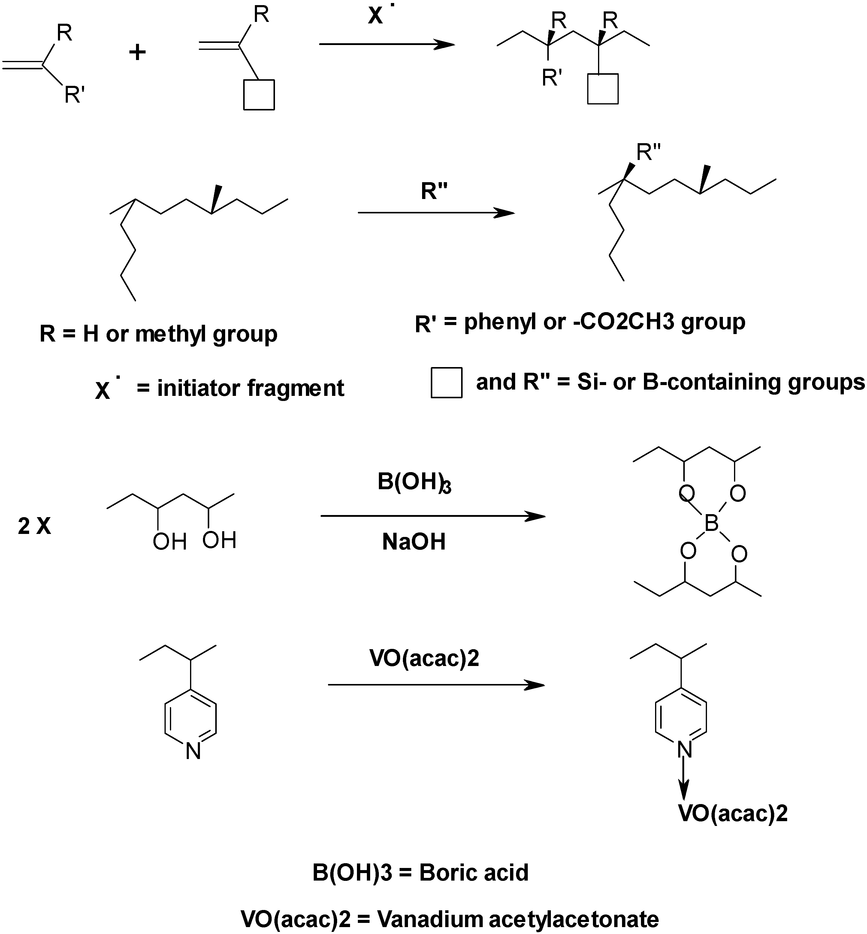
- Ebdon, J.R.; Hunt, B.J.; Jones, M.S.; Thorpe, F.G. Chemical modification of polymers to improve flame retardance—II: The influence of silicon-containing groups. Polym. Degrad. Stab. 1996, 69, 395–400. [Google Scholar] [CrossRef]
- Ebdon, J.R.; Guisti, L.; Hunt, B.J.; Jones, M. The effects of some transition-metal compounds on the flame retardance of poly(styrene-co-4-vinyl pyridine) and poly(methyl methacrylate-co-4-vinyl pyridine). Polym. Degrad. Stab. 1998, 60, 401–407. [Google Scholar] [CrossRef]
- Armitage, P.; Ebdon, J.R.; Hunt, B.J.; Jones, M.S.; Thorpe, F.G. Chemical modification of polymers to improve flame retardance—I. The influence of boron-containing groups. Polym. Degrad. Stab. 1996, 54, 387–393. [Google Scholar] [CrossRef]
- Ebdon, J.R.; Price, D.B.; Hunt, B.J.; Joseph, P.; Gao, F.; Milnes, G.J.; Cunliffe, L.K. Flame retardance in some polystyrenes and poly(methyl methacrylate)s with covalently bound phosphorus-containing groups: initial screening experiments and some laser pyrolysis mechanistic studies. Polym. Degrad. Stab. 2000, 69, 267–277. [Google Scholar] [CrossRef]
- Ebdon, J.R.; Hunt, B.J.; Joseph, P. Thermal degradation and flammability characteristics of some polystyrenes and poly(methyl methacrylate)s chemically modified with silicon-containing groups. Polym. Degrad. Stab. 2004, 83, 181–185. [Google Scholar] [CrossRef]
- Zhang, S.; Hull, T.R.; Horrocks, A.R.; Smart, G.; Kandola, B.K.; Ebdon, J.; Hunt, B.; Joseph, P. Thermal degradation analysis and XRD characterisation of fibre-forming synthetic polypropylene containing nanoclay. Polym. Degrad. Stab. 2007, 92, 727–732. [Google Scholar] [CrossRef]
- Marxman, G.A.; Gilbert, M. Turbulent boundary layer combustion in the hybrid rocket. In Ninth International Symposium on Combustion; Academic Press: New York, NY, USA, 1963; pp. 371–383. [Google Scholar]
- Marxman, G.A.; Wooldridge, C.E.; Muzzy, R.J. Fundamentals of hybrid boundary layer combustion. In Heterogeneous Combustion (AIAA Progress in Astronautics and Aeronautics); Wolfhard, H.G., Glassman, I., Green, L., Jr., Eds.; Academic Press: New York, NY, USA, 1964; Volume 15, pp. 485–521. [Google Scholar]
- Chiaverini, M.J. Review of solid-fuel regression rate behavior in classical and nonclassical hybrid rocket motors. In Fundamentals of Hybrid Rocket Combustion and Propulsion (Progress in Astronautics and Aeronautics); Chiaverini, M.J., Kuo, K.K., Eds.; AIAA: Reston, VA, USA, 2007; Volume 218, pp. 37–125. [Google Scholar]
- Lengelle, G. Solid-fuel pyrolysis phenomena and regression rate. In Fundamentals of Hybrid Rocket Combustion and Propulsion (Progress in Astronautics and Aeronautics); Chiaverini, M.J., Kuo, K.K., Eds.; AIAA: Reston, VA, USA, 2007; Volume 218, pp. 127–165. [Google Scholar]
- Zeng, W.R.; Li, S.F.; Chow, W.K. Review on chemical reactions of burning poly(methylmethacrylate) PMMA. J. Fire Sci. 2002, 20, 401–433. [Google Scholar] [CrossRef]
- Ananth, R.; Ndubizu, C.C.; Tatem, P.A. Burning rate distributions for boundary layer flow combustion of a PMMA plate in forced flow. Combust. Flame 2003, 135, 35–55. [Google Scholar] [CrossRef]
- Stoliarov, S.I.; Crowley, S.; Lyon, R.E.; Linteris, G.T. Prediction of the burning rates of non-charring polymers. Combust. Flame 2009, 156, 1068–1083. [Google Scholar] [CrossRef]
- Arisawa, H.; Brill, T.B. Kinetics and mechanisms of flash pyrolysis of poly(methyl methacrylate) (PMMA). Combust. Flame 1997, 109, 415–426. [Google Scholar] [CrossRef]
- Bedir, H.; T’ien, J.S. A Computational Study of Flame Radiation in PMMA Diffusion Flames Including Fuel Vapor Participation. In Proceedings of the Twenty-Seventh Symposium (International) on Combustion, Combustion Institute, Pittsburgh, PA, USA, 2–7 August 1998; Volume 27, pp. 2821–2828.
- Vovelle, C.; Delfau, J.L.; Reuillon, M.; Bransier, J.; Laraqui, N. Experimental and numerical study of the thermal degradation of PMMA. Combust. Sci. Technol. 1987, 53, 187–207. [Google Scholar] [CrossRef]
- Krishnamurthy, L.; Williams, F.A. Fourteenth Symposium (International) on Combustion; The Combustion Institute: Pittsburgh, PA, USA, 1974. [Google Scholar]
- Kashiwagi, T.H.; Brown, J.E. Thermal and oxidative degradation of poly(methyl methacrylate) molecular weight. Macromolecules 1985, 18, 131–138. [Google Scholar] [CrossRef]
- Kumar, R.N.; Stickler, D.B. Polymer-degradation theory of pressure-sensitive hybrid combustion. Proc. Symp. (Int.) Combust. 1971, 13, 1059–1072. [Google Scholar] [CrossRef]
- Madorsky, S.L. Thermal Degradation of Organic Polymers; Interscience Publishers: New York, NY, USA, 1964. [Google Scholar]
- Zeng, W.R.; Li, S.F.; Chow, W.K. Preliminary studies on burning behavior of poly(methylmethacrylate) (PMMA). J. Fire Sci. 2002, 20, 297–317. [Google Scholar] [CrossRef]
- GRI-MECH Database Homepage. Available online: http://www.me.berkeley.edu/gri-mech/ (accessed on 21 October 2011).
- Bell, K.M.; Tipper, C.F.H. The slow combustion of methylalcohol, a general investigation. Proc. R. Soc. Lond. Ser. A 1956, 238, 256–268. [Google Scholar] [CrossRef]
- Vardanyan, I.A.; Sachyan, G.A.; Nalbandyan, A.B. Kinetics and mechanism of formaldehyde oxidation. Combust. Flame 1971, 17, 315–322. [Google Scholar] [CrossRef]
- Hay, J.M.; Hessam, K. The oxidation of gaseous formaldehyde. Combust. Flame 1971, 16, 237–242. [Google Scholar] [CrossRef]
- Hidaka, Y.; Hattori, K.; Okuno, T.; Inami, K.; ABE, T.; Koike, T. Shock-tube and modeling study of acetylene pyrolysis and oxidation. Combust. Flame 1996, 107, 401–417. [Google Scholar] [CrossRef]
- Wilkie, C.A. TGA/FTIR: An extremely useful technique for studying polymer degradation. Polym. Degrad. Stab. 1999, 66, 301–306. [Google Scholar] [CrossRef]
- Raemaekers, K.G.H.; Bart, J.C.J. Applications of simultaneous thermogravimetry-mass spectrometry in polymer analysis. Thermochim. Acta 1997, 295, 1–58. [Google Scholar] [CrossRef]
- Kaisersberger, E.; Post, E. Practical aspects for the coupling of gas analytical methods with thermal-analysis instruments. Thermochim. Acta 1997, 295, 73–93. [Google Scholar] [CrossRef]
- Maciejewski, M.; Baiker, A. Quantitative calibration of mass spectrometric signals measured in coupled TA-MS system. Thermochim. Acta 1997, 295, 95–105. [Google Scholar] [CrossRef]
- Marsanich, K.; Barontini, F.; Cozzani, V.; Petarca, L. Advanced pulse calibration techniques for the quantitative analysis of TG-FTIR data. Thermochim. Acta 2002, 390, 153–168. [Google Scholar] [CrossRef]
- Branley, N.; Jones, W.P. Large eddy simulation of a turbulent non- premixed flame. Combust. Flame 2001, 127, 1914–1934. [Google Scholar] [CrossRef]
- Peters, N. Laminar diffusion flamelet models in non-premixed turbulent combustion. Prog. Energy Combust. Sci. 1984, 10, 319–339. [Google Scholar] [CrossRef]
- Pitsch, H.; Chen, M.; Peters, N. Unsteady flamelet modeling of turbulent hydrogen-air diffusion flames. Proc. Symp. (Int.) Combust. 1998, 27, 1057–1064. [Google Scholar] [CrossRef]
- Pitsch, H.; Cha, C.M.; Fedotov, S. Interacting Flamelet Model for Non-Premixed Turbulent Combustion with Local Extinction and Re-Ignition; Annual Research Briefs 2001; Center for Turbulence Research, Stanford University: Menlo Park, CA, USA, 2001. [Google Scholar]
- Pitsch, H.; Peters, N. A consistent flamelet formulation for non-premixed combustion considering differential diffusion effects. Combust. Flame 1998, 114, 26–40. [Google Scholar] [CrossRef]
- Gran, I.R.; Melaaen, M.C.; Magnussen, B.F. Numerical simulation of local extinction effects in turbulent combustor flows of methane and air. Proc. Symp. (Int.) Combust. 1994, 25, 1283–1291. [Google Scholar] [CrossRef]
- Pantano, C.; Sarkar, S.; Williams, F.A. Mixing of a conserved scalar in a turbulent reacting shear layer. J. Fluid Mech. 2003, 481, 291–328. [Google Scholar] [CrossRef]
- Pitsch, H. Extended Flamelet Model for LES of Non-Premixed Combustion; Annual Research Briefs 2000; Center for Turbulence Research, Stanford University: Menlo Park, CA, USA, 2000. [Google Scholar]
- Chiaverini, M.J.; Serin, N.; Johnson, D.K.; Lu, Y.; Kuo, K.K.; Risha, G.A. Regression rate behavior of hybrid rocket solid fuels. J. Propul. Power 2000, 16, 125–132. [Google Scholar] [CrossRef]
- Sankaran, V. Computational fluid dynamics modeling of hybrid rocket flowfields. In Fundamentals of Hybrid Rocket Combustion and Propulsion (Progress in Astronautics and Aeronautics); Chiaverini, M.J., Kuo, K.K., Eds.; AIAA: Reston, VA, USA, 2007; Volume 218, pp. 323–349. [Google Scholar]
- Hossain, M.; Jones, J.C.; Malalasekera, W. Modelling of a bluff-body nonpremixed flame using a coupled radiation/flamelet combustion model. Flow Turbul. Combust. 2001, 67, 217–234. [Google Scholar] [CrossRef]
- Novozhilov, V. Computational fluid dynamics modelling of compartment fires. Prog. Energy Combust. Sci. 2001, 27, 611–666. [Google Scholar] [CrossRef]
- Lockwood, F.C.; Shah, N.G. A new radiation solution method for incorporation in general combustion prediction procedures. Proc. Symp. (Int.) Combust. 1981, 18, 1405–1414. [Google Scholar] [CrossRef]
- Novozhilov, V.; Harvie, D.J.E.; Kent, J.H.; Apte, V.B.; Pearson, D. A computational fluid dynamics study of wood fire extinguishment by water sprinkler. Fire Saf. J. 1997, 29, 259–282. [Google Scholar] [CrossRef]
- Novozhilov, V.; Harvie, D.J.E.; Green, A.R.; Kent, J.H. A computational fluid dynamic model of fire burning rate and extinction by water sprinkler. Combust. Sci. Technol. 1997, 123, 227–245. [Google Scholar] [CrossRef]
- Kuo, K.K. Principles of Combustion; Wiley: New York, NY, USA, 1986. [Google Scholar]
- Gosman, A.D.; Ioannides, E. Aspects of computer simulation of liquid-fuelled combustors. In Proceedings of the American Institute of Aeronautics and Astronautics, Aerospace Sciences Meeting, St. Louis, MO, USA, 12–15 January 1981.
- Faeth, G.M. Evaporation and combustion of sprays. Prog. Energy Combust. Sci. 1983, 9, 1–76. [Google Scholar] [CrossRef]
- Crowe, C.T.; Sharma, M.P.; Stock, D.E. Theparticle-source-incell(PSI Cell) model for gas-droplet flows. J. Fluids Eng. 1977, 99, 325–332. [Google Scholar] [CrossRef]
- Crowe, C.T. Heat transfer in dispersed-phase flow. In Two Phase Momentum, Heat and Mass Transfer in Chemical, Process and Energy Engineering Systems; Afgan, N.H., Tsiklauri, G.V., Eds.; Hemisphere: McGraw-Hill: New York, NY, USA, 1978; Volume 1, pp. 23–32. [Google Scholar]
- Shuen, J.S.; Chen, L.D.; Faeth, G.M. Evaluation of a stochastic model of particle dispersion in a turbulent round jet. AIChE J. 1983, 29, 167–170. [Google Scholar] [CrossRef]
- Shuen, J.S.; Chen, L.D.; Faeth, G.M. Predictions of the structure of turbulent, particle. Laden, round jets. AIAA J. 1983, 21, 1483–1484. [Google Scholar] [CrossRef]
- Novozhilov, V. On some integrable cases of particle motion in a fluid, mathematics in engineering. Sci. Aerosp. 2010, 1, 371–380. [Google Scholar]
- Novozhilov, V. Flashover control under fire suppression conditions. Fire Saf. J. 2001, 36, 641–660. [Google Scholar] [CrossRef]
- Putnam, A. Integrable form of droplet drag coefficient. Am. Rocket Soc. J. 1961, 31, 1467–1468. [Google Scholar]
- Faeth, G.M. Evaporation and Combustion of Sprays. Prog. Energy Combust. Sci. 1983, 9, 1–76. [Google Scholar] [CrossRef]
- Shirolkar, J.S.; Coimbra, C.F.M.; McQuay, M.Q. Fundamental aspects of modeling turbulent particle dispersion in dilute flows. Progr. Energy Combust. Sci. 1993, 22, 363–399. [Google Scholar] [CrossRef]
- Ranz, W.E.; Marshall, W.R., Jr. Evaporation from drops: Part I. Chem. Eng. Progress. 1952, 48, 141–146. [Google Scholar]
- Ranz, W.E.; Marshall, W.R., Jr. Evaporation from drops: Part II. Chem. Eng. Progress. 1952, 48, 173–180. [Google Scholar]
- Faeth, G.M.; Lazar, R.S. Fuel droplet burning rates in a combustion gas environment. AIAA J. 1971, 9, 2165–2171. [Google Scholar] [CrossRef]
- Migdal, D.; Agosta, V.D. A Source Flow Model for Continuum Gas-Particle Flow. J. Appl. Mech. 1967, 34, 860–865. [Google Scholar] [CrossRef]
- Kumar, S.; Heywood, G.M.; Liew, S.K. Superdrop Modelling of a Sprinkler Spray in a Two-phase Cfdparticle Tracking Model. In Proceedings of the Fifth International Symposium on Fire Safety Science, Melbourne, Australia, 3–7 March 1997; pp. 889–900.
- Lin, C.L.; Chiu, H.H. Numerical Analysis of Spray Combustion in Hybrid Rocket, AIAA 95-2687. In Proceedings of the 31st AIANASMUSAUASEE Joint Propulsion Conference and Exhibition, San Diego, CA, USA, 1995.
- Kawamura, T.; Kuwahara, K. Computation of High Reynolds Number Flow Around A Circular Cylinder with Surface Roughness. In Proceedings of the 22nd American Institute of Aeronautics and Astronautics, Aerospace Sciences Meeting, Reno, NV, USA, 9–12 January 1984.
- Boris, J.P.; Grinstein, F.F.; Oran, E.S.; Kolbe, R.L. New insights into large eddy simulation. Fluid Dyn. Res. 1992, 10, 199–228. [Google Scholar] [CrossRef]
- van Leer, B. Towards the ultimate conservative difference scheme V: A second-order sequel to Godunov’s method. J. Computat. Phys. 1979, 32, 101–136. [Google Scholar] [CrossRef]
- Shu, C.W.; Osher, S. Efficient implementation of essentially non-oscillatory shock-capturing schemes, I. J. Comput. Phys. 1988, 77, 439–471. [Google Scholar] [CrossRef]
- Shu, C.W.; Osher, S. Efficient implementation of essentially non-oscillatory shock-capturing schemes, II. J. Comput. Phys. 1989, 83, 32–78. [Google Scholar] [CrossRef]
- Liu, X.D.; Osher, S.; Chan, T. Weighted essentially non-oscillatory schemes. J. Comput. Phys. 1994, 115, 200–212. [Google Scholar] [CrossRef]
- Jiang, G.S.; Shu, C.W. Efficient implementation of weighted ENO schemes. J. Comput. Phys. 1996, 126, 202–228. [Google Scholar] [CrossRef]
- Deng, X.G.; Zhang, H.X. Developing high-order weighted compact nonlinear schemes. J. Comput. Phys. 2000, 165, 22–44. [Google Scholar] [CrossRef]
- Drikakis, D.; Hahn, M.; Mosedale, A.; Thornber, B. Large eddy simulation using high-resolution and high-order methods. Philos. Trans. R. Soc. A 2009, 367, 2985–2997. [Google Scholar] [CrossRef] [PubMed]
- Hahn, M.; Drikakis, D. Implicit large-eddy simulation of swept-wing flow using high-resolution methods. AIAA J. 2009, 47, 618–630. [Google Scholar] [CrossRef]
- Panaras, A.G.; Drikakis, D. High-speed unsteady flows around spiked-blunt bodies. J. Fluid Mech. 2009, 632, 69–96. [Google Scholar] [CrossRef]
- Shimada, Y.; Thornber, B.; Drikakis, D. High-order implicit large eddy simulation of gaseous fuel injection and mixing of a bluff body burner. Comput. Fluids 2011, 44, 229–237. [Google Scholar] [CrossRef]
- Gordon, S.; McBride, B.J. Computer Program for Calculation of Complex Chemical Equilibrium Compositions and Applications, II. Users Manual and Program Description; Nasa Reference Publication 1311; Lewis Research Center: Cleveland, OH, USA, 1996. [Google Scholar]
- Liou, M.S.; Steffen, C.J., Jr. A new flux splitting scheme. J. Comput. Phys. 1993, 107, 23–39. [Google Scholar] [CrossRef]
- Liou, M.S. A sequel to AUSM, Part II: AUSM+-up for all speeds. J. Comput. Phys. 2006, 214, 137–170. [Google Scholar] [CrossRef]
- Shima, E.; Kitamura, K. On New Simple Low-Dissipation Scheme of AUSM-Family for All Speeds; AIAA Paper 2009-136; AIAA: Reston, VA, USA, 2009. [Google Scholar]
- Roe, P.L. Characteristic-based schemes for the Euler equations. Annu. Rev. Fluid Mech. 1986, 18, 337–365. [Google Scholar] [CrossRef]
- van Leer, B. Towards the ultimate conservative difference scheme II: Monotonicity and conservation combined in a second-order scheme. J. Comput. Phys. 1974, 14, 361–370. [Google Scholar] [CrossRef]
- Anderson, W.K.; Thomas, J.L.; van Leer, B. A Comparison of Finite Volume Flux Vector Splittings for the Euler Equations; AIAA Paper 85-122; AIAA: Reston, VA, USA, 1985. [Google Scholar]
© 2011 by the authors; licensee MDPI, Basel, Switzerland. This article is an open access article distributed under the terms and conditions of the Creative Commons Attribution license (http://creativecommons.org/licenses/by/3.0/).
Share and Cite
Novozhilov, V.; Joseph, P.; Ishiko, K.; Shimada, T.; Wang, H.; Liu, J. Polymer Combustion as a Basis for Hybrid Propulsion: A Comprehensive Review and New Numerical Approaches. Energies 2011, 4, 1779-1839. https://doi.org/10.3390/en4101779
Novozhilov V, Joseph P, Ishiko K, Shimada T, Wang H, Liu J. Polymer Combustion as a Basis for Hybrid Propulsion: A Comprehensive Review and New Numerical Approaches. Energies. 2011; 4(10):1779-1839. https://doi.org/10.3390/en4101779
Chicago/Turabian StyleNovozhilov, Vasily, Paul Joseph, Keiichi Ishiko, Toru Shimada, Hui Wang, and Jun Liu. 2011. "Polymer Combustion as a Basis for Hybrid Propulsion: A Comprehensive Review and New Numerical Approaches" Energies 4, no. 10: 1779-1839. https://doi.org/10.3390/en4101779
APA StyleNovozhilov, V., Joseph, P., Ishiko, K., Shimada, T., Wang, H., & Liu, J. (2011). Polymer Combustion as a Basis for Hybrid Propulsion: A Comprehensive Review and New Numerical Approaches. Energies, 4(10), 1779-1839. https://doi.org/10.3390/en4101779