Article

Battery Health Prediction with Singular Spectrum Analysis and Grey Wolf Optimized Long Short-Term Memory Networks

1
College of Engineering, Huaqiao University, Quanzhou 362021, China
2
Business School, Huaqiao University, Quanzhou 362021, China
3
College of Transportation and Navigation, Quanzhou Normal University, Quanzhou 362000, China
*
Author to whom correspondence should be addressed.
These authors contributed equally to this work.
Energies 2025, 18(9), 2401; https://doi.org/10.3390/en18092401
Submission received: 8 April 2025 / Revised: 1 May 2025 / Accepted: 4 May 2025 / Published: 7 May 2025

Abstract

:
To tackle the intricate challenges of nonlinearity and non-stationarity in lead-acid battery degradation data, this paper introduces the SG-LSTM model, an innovative approach to battery health prediction. This model uniquely integrates Singular Spectrum Analysis (SSA) and Grey Wolf Optimization (GWO) with Long Short-Term Memory (LSTM) networks, forming a sophisticated predictive framework. By targeting key degradation features, such as the charging time of multiple voltage rise segments from the charging curve, the model effectively captures critical battery health dynamics. SSA plays a vital role by filtering outliers from these feature sequences, ensuring high-quality data for analysis and enhancing the robustness and accuracy of predictions. The refined data are then processed by a GWO-optimized LSTM network, where GWO’s bio-inspired optimization fine-tunes the LSTM parameters for optimal performance. Experimental results demonstrate that the SG-LSTM model outperforms existing models in prediction accuracy and stability; specifically, SG-LSTM achieves 0.27 RMSE, outperforming LSTM (0.84), SSA-LSTM (0.4), and SSA-BP (0.6).

1. Introduction

Lead-acid batteries are widely utilized in diverse applications, including automotive, railway, marine, and telecommunications industries, and backup power systems, due to their low cost and superior high-rate discharge performance. For systems that use lead-acid batteries, the State of Health (SOH) of these batteries critically influences overall system stability. Therefore, accurate SOH assessment is essential. Currently, research on the health status of lead-acid batteries remains significantly less extensive compared to that on lithium-ion batteries; hence, methodologies developed for lithium batteries will be referenced in this study. Methods for predicting battery health status primarily fall into two categories: model-driven and data-driven approaches [1,2,3,4,5]. Model-driven methods mainly rely on battery physical mechanism models or empirical degradation models. Physical mechanism models usually require an in-depth understanding of the battery’s internal electrochemical mechanisms to establish the relationship between model parameters and SOH from the physical mechanism of batteries [6]. Empirical degradation models, such as those utilizing the ampere-hour integral method or internal resistance measurements, analyze historical capacity fade trends or quantitatively estimate remaining capacity to assess battery health [7,8,9]. Data-driven methods, by contrast, bypass the explicit modeling of internal degradation mechanisms. Instead, these approaches extract features indicative of capacity fade (e.g., voltage/current profiles during charge–discharge cycles) from operational data and construct predictive mappings between these features and SOH through machine learning. Based on the multi-phase Weiner process degradation model, Yang et al. [10] proposed a prediction method for lead-acid battery health state estimation and Remaining Useful Life (RUL). However, the Weiner process assumes that the degradation noise is a Gaussian distribution, but in fact the battery degradation may have non-Gaussian noise or mutation phenomenon, which may affect the prediction accuracy. Sun et al. [11] utilized Convolutional Neural Networks (CNNs) to extract local spatial features such as voltage from battery charge and discharge data. By employing Bidirectional Long Short-Term Memory (BiLSTM) networks to capture temporal dependencies, they introduced attention mechanisms to dynamically weight the importance of features at different time steps, thereby enhancing the model’s sensitivity to degradation features. Yu et al. [12] proposed a Time-series Convolutional Network (TCN) model based on multi-health feature extraction and Particle Swarm Optimization (PSO). The high accuracy and robustness of this method in different training datasets and lithium battery systems were verified by experiments. Fu et al. [13] proposed a VMD-PE-IDBO-TCN prediction model, which used the method of VMD combined with Permutation Entropy (PE) to reconstruct the original lithium battery SOH data and used the Improved Dung Beetle Optimization (IDBO) algorithm to optimize the hyperparameters of the TCN model, so as to achieve high precision SOH prediction. Xu et al. [14] proposed a hybrid method combining the Transformer model with the Unscented Particle Filter (UPF) to predict the health status of lithium-ion batteries. By leveraging the global prediction capability of Transformer and the online correction capability of the UPF-based local correction model, high-precision battery health predictions can be achieved under different aging conditions. Guijun Ma et al. [15] employed convolutional neural networks to automatically extract features from raw charging voltage curves and implemented transfer learning for the personalized SOH estimation of new batteries. Winata et al. [16] used three machine-learning algorithms—Gaussian Process Regression, Support Vector Machine, and Random Forest—to predict the degradation of lead-acid batteries based on real-time monitored voltage and temperature as features and proved that Random Forest had the best prediction performance. Zhang et al. [17] used a Long Short-Term Memory (LSTM) recurrent neural network to capture long-term dependencies in lithium-ion battery capacity fade, optimizing their model with resilient mean square back-propagation and dropout techniques. Overall, data-driven methods have gained prominence due to their ability to circumvent complex battery modeling. These techniques typically exploit machine learning to uncover latent relationships between measurable battery parameters (e.g., voltage, current) and internal health states, thereby enabling robust SOH prediction.
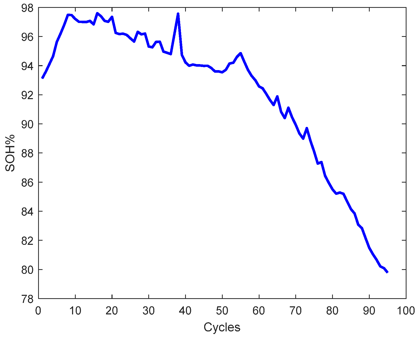
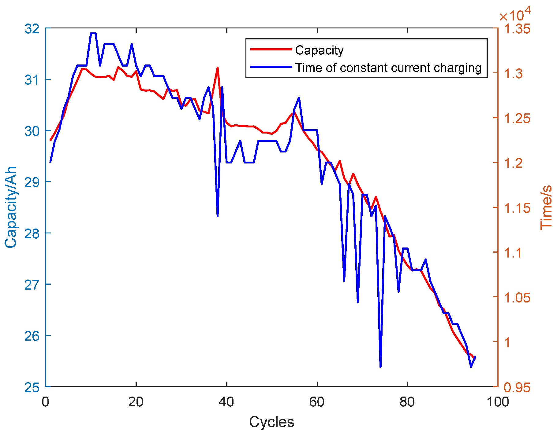
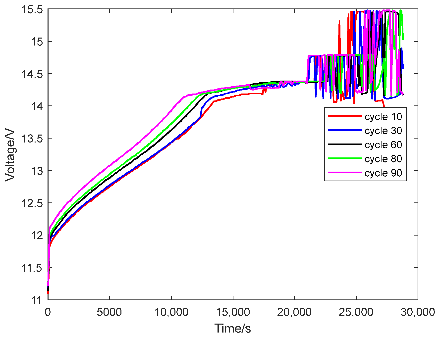
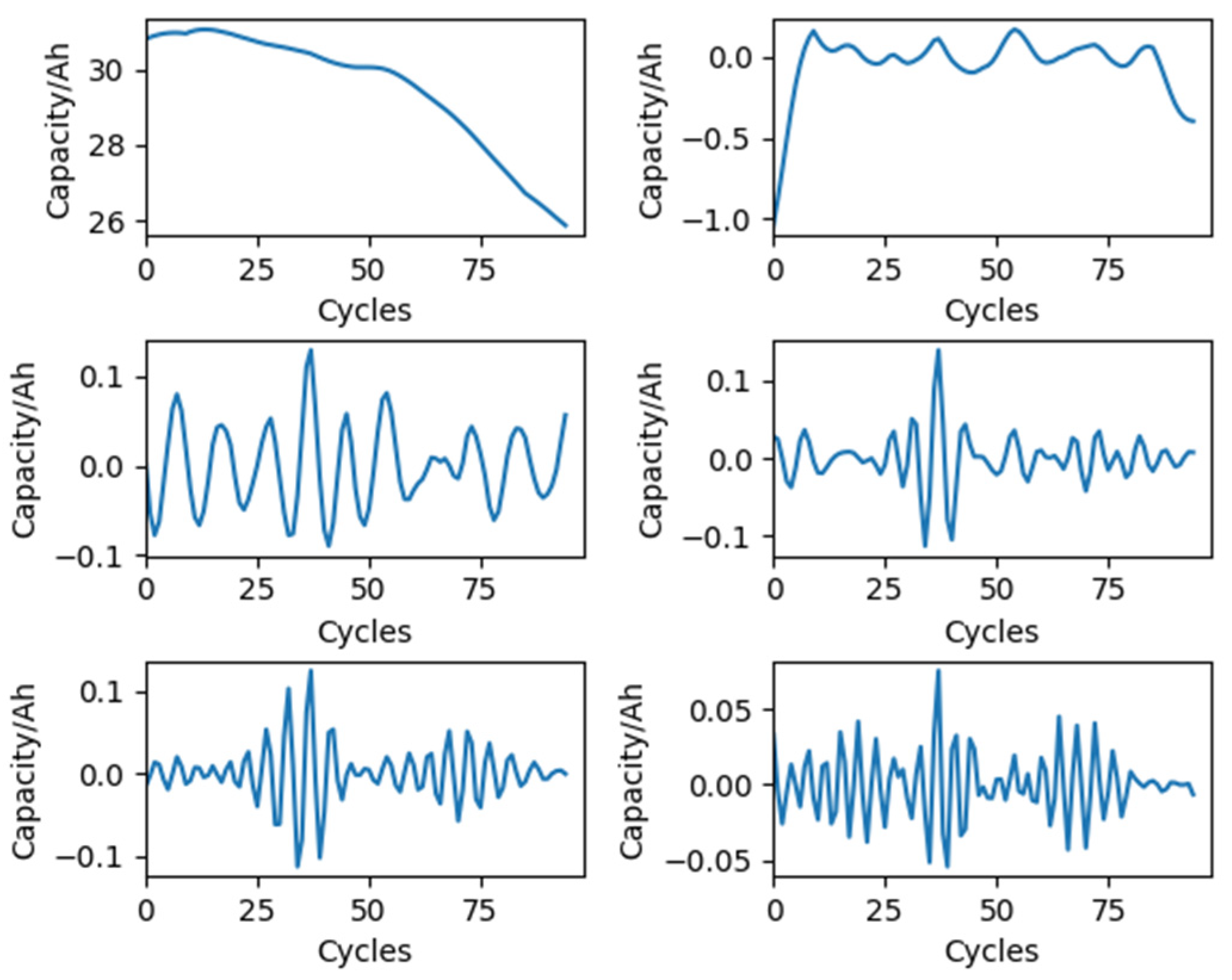
The capacity degradation of lead-acid batteries stems from their internal electrochemical mechanisms, resulting in nonlinear and non-stationary degradation data. This inherent complexity poses significant challenges for accurate battery health status prediction. The operational data collected during battery cycling can be characterized as nonlinear and non-stationary time series. To maximize information extraction while mitigating noise interference, researchers often decompose such time series into multiple components with distinct temporal scales. Subsequent analysis and recombination of these individual components enable effective noise separation [18]. Singular Spectrum Analysis (SSA) is an efficient method for processing non-stationary time-series data [19]. The ability of SSA to separate noise, trend, and harmonic is consistent with the physical degradation of lead-acid batteries and can perform interpretable feature extraction. Requiring no prior assumptions, SSA preserves critical data features while demonstrating superior noise suppression capabilities compared to Empirical Mode Decomposition (EMD) and wavelet decomposition, as evidenced in [20,21].
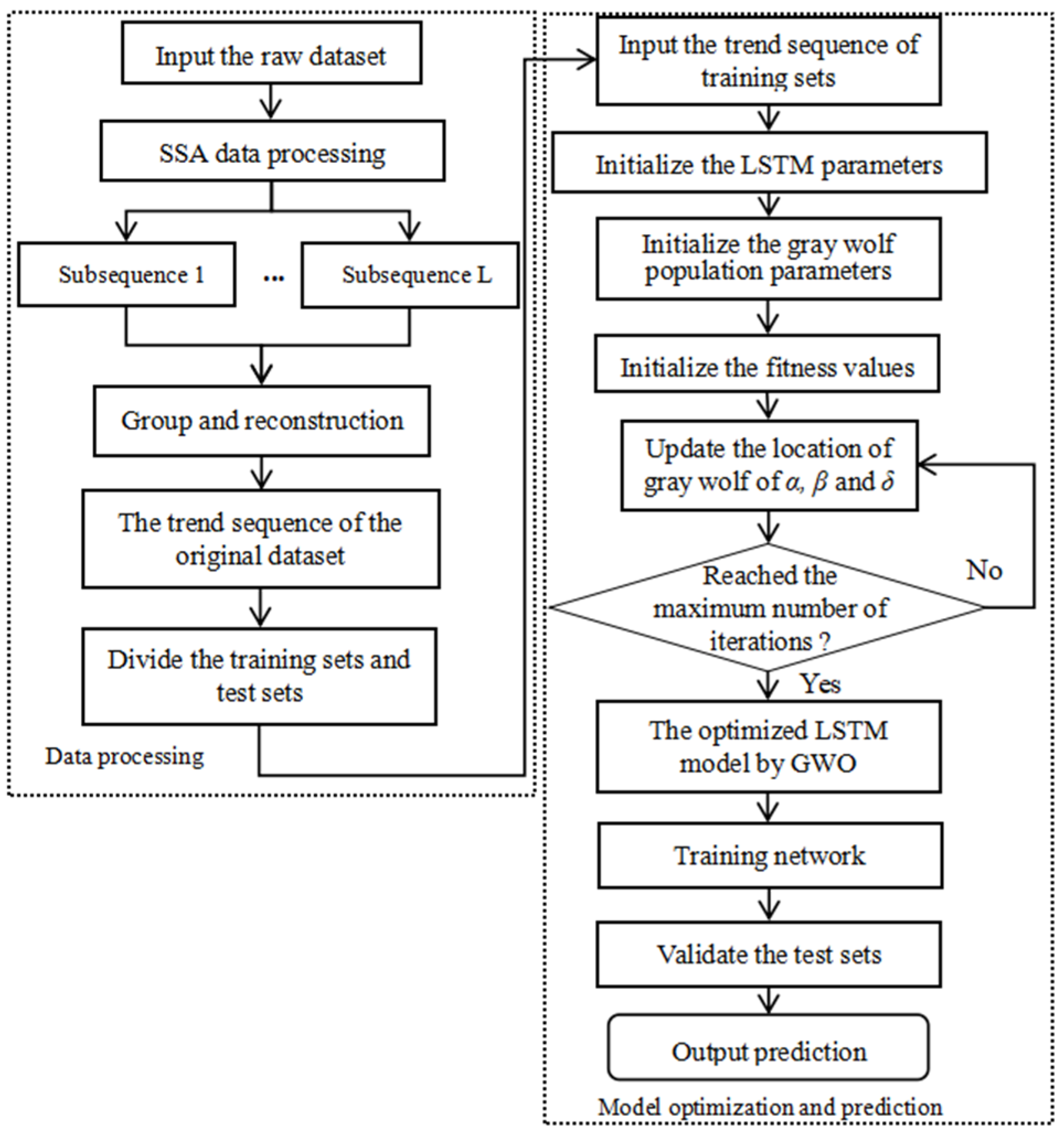
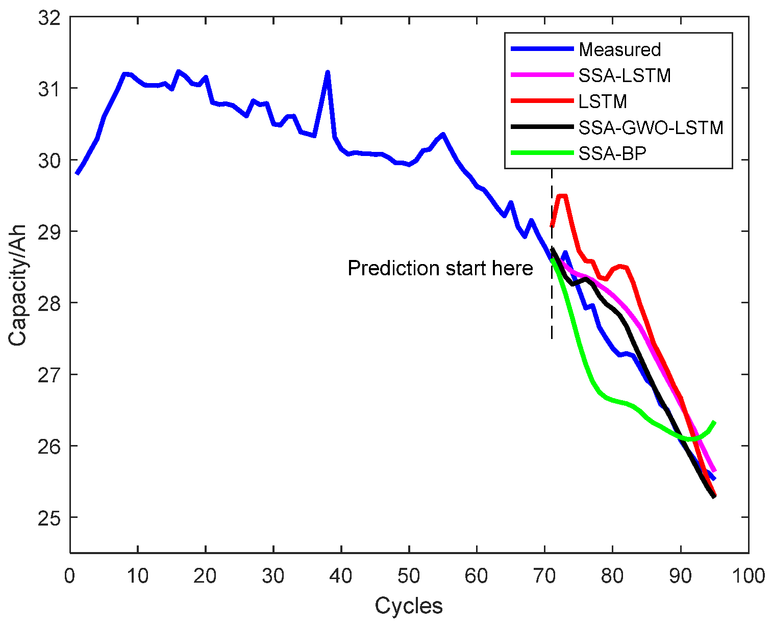
Based on the preceding analysis, this study employs a data-driven approach to evaluate the SOH of lead-acid batteries. To enhance prediction accuracy, the singular spectral analysis is integrated to preprocess the sequence of degradation features. Subsequently, the processed data are fed into an LSTM network for model training and prediction.
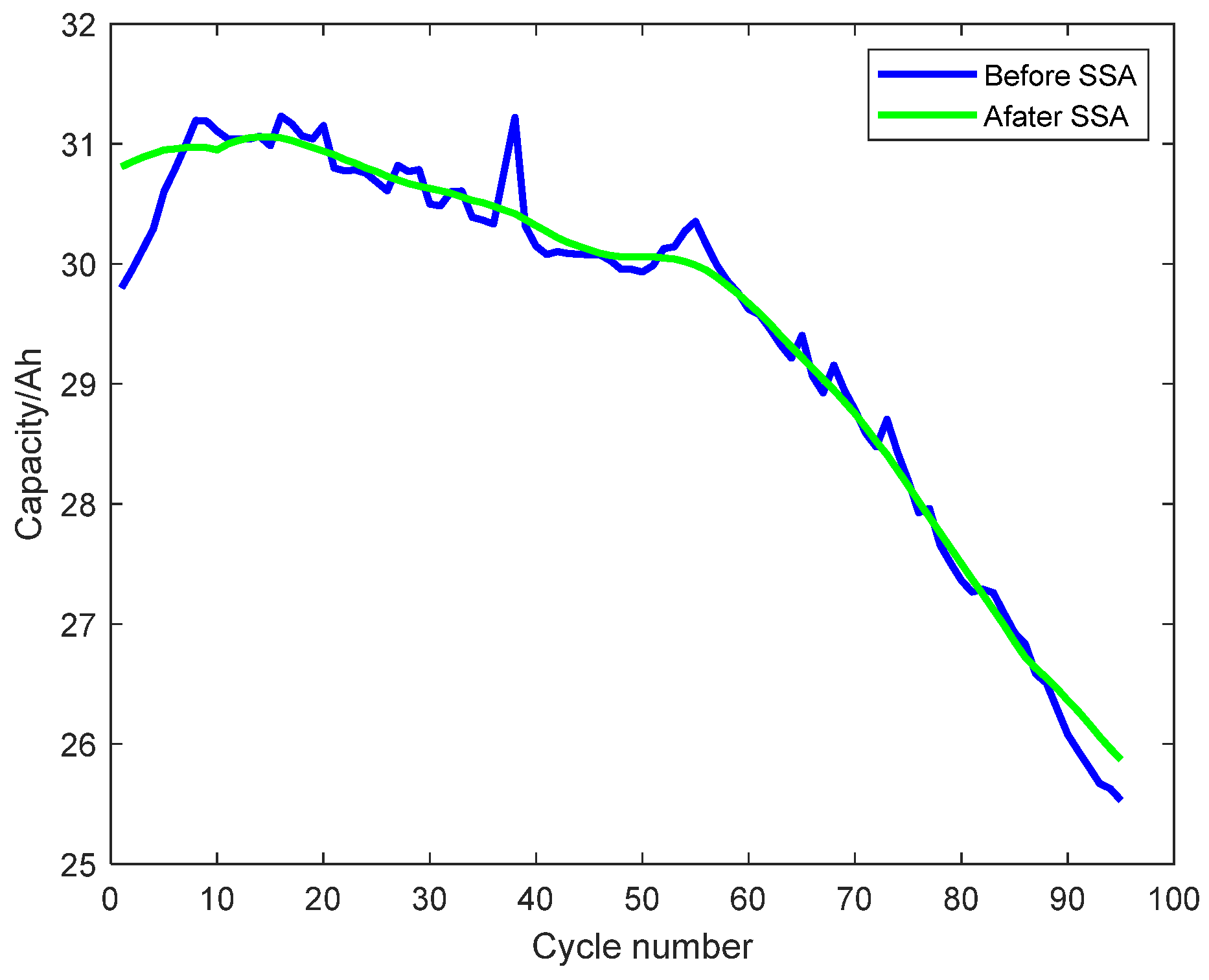
Our main contributions are as follows: (i) Combining the SSA method with the LSTM network algorithm to form an efficient SOH prediction model; (ii) Using the SSA method to preprocess battery capacity degradation data and extract the trend sequence of the data, which makes the characteristics of the data more significant; (iii) Optimizing the parameters of the LSTM network by using the Grey Wolf Optimization (GWO) algorithm, improving the robustness and accuracy of the model.
The rest of this paper is organized as follows: Section 2 introduces the principles of several of the algorithms used and their applications in battery health status estimation and provides indicators for evaluating model performance. Section 3 introduces the data used in the experiment and the process of extracting and selecting health indicators from the original data. Section 4 compares the predictive effect of various algorithms through experiments, and the relevant work of this paper is summarized and discussed in Section 5.

2. Methods

In this section, we first introduce the principle of the SSA method and then elaborate on the method of using the GWO algorithm to optimize the parameters of the LSTM network. Finally, the performance indicators are given for evaluating the model.

2.1. Singular Spectrum Analysis

Singular spectrum analysis is a powerful denoising technique widely applied to time-series analysis; it can extract nonlinear trends, periodic oscillations, and noise signals from observational data. During the process of collecting battery data, due to the influence of factors such as the performance of sensors and the working environment, the measured data need to be denoised. SSA mainly includes decomposition and reconstruction processes [22], implemented as follows:
(1)
Embedding
The original one-dimensional sequence [X1, X2, …, XN] with length N is slid according to a suitable window L, generally L < N/2, to form multiple sub-sequences, and these sub-sequences are arranged as rows or columns of a matrix with dimensions L × K to obtain a trajectory matrix, as shown in Equation (1):
X = x 1 x 2 x K x 2 x 3 x K + 1 x L x L + 1 x N
where K = NL + 1.
(2)
Singular Value Decomposition (SVD)
Singular value decomposition for X and sorting it in descending order. Through eigenvalue decomposition of the covariance matrix C = XXT of X, the eigenvectors U1, U2, …, UL corresponding to the eigenvalues λ1 > λ2 > … > λL ≥ 0 are obtained. Using the SVD method, the trajectory matrix of X is transformed into:
X = i = 1 d λ i U i V i T
where d = max ( i , λ i > 0 ) = r a n k ( X ) represents the number of non-zero singular values and λ i represents the singular values of the time series X. Ui and Vi are the left and right eigenvectors of the covariance matrix C, respectively. λ i U i V i T is the elementary matrix. The largest eigenvalue corresponds to the largest eigenvector, which represents the direction of maximum change, while the eigenvectors corresponding to smaller eigenvalues are usually considered noise.
(3)
Grouping
If data X are composed of useful signal S and noise E, that is, X = S + E, grouping removes E from the data as much as possible. The first r larger singular values are considered as useful data, and the remaining d-r part is noise, so that the useful data and noise can be separated by selecting an appropriate r value.
(4)
Reconstruction
Reconstruction uses the diagonal averaging formula to transform the grouped matrix into the Reconstruction Components (RC) with a length of N. Let Y R L × K represent any matrix obtained after grouping and yij (1 ≦ iL, 1 ≦ jK) represent the elements in the matrix. L * = min ( L , K ) , K = max ( L , K ) , if L < K, y i j * = y i j , otherwise y i j * = y j i . Therefore, the matrix Y can be transformed into the required sequence with a length of N by the diagonal averaging method, y r c 1 , y r c 2 , , y r c N ; the relevant Equation is as follows:
y r c k = 1 k m = 1 k y m , k m + 1 * 1 k < L * 1 L * m = 1 L * y m , k m + 1 * 1 k K * 1 N k + 1 m = k K * + 1 N K * + 1 y m , k m + 1 * K * < k N
where y r c k is the k-th sequence transformed by diagonal averaging and y i j * is the element in the matrix.

2.2. Grey Wolf Optimization Algorithm

The Grey Wolf Optimization Algorithm is a swarm intelligence algorithm proposed by Mirjalili et al. in 2014 that simulates the hierarchical structure and hunting behavior of grey wolf packs [23]. The GWO algorithm is characterized by its simple structure, few parameters that need to be adjusted, and easy implementation, and it has been widely applied in research fields such as machine learning, image processing, and networks [24,25]. In the GWO framework, grey wolves are classified into four hierarchical levels: the α wolf (leader), β wolf (second-in-command), δ wolf (scout/hunter), and ω wolves (followers). The β wolf assists the α in decision-making, while the δ wolf is responsible for scouting, hunting, and maintaining pack safety. The ω wolves, representing the majority of the pack, follow the directives of the higher-ranked wolves. During optimization, the first three levels (α, β, δ) guide the ω wolves to search for prey (i.e., optimal solutions). The GWO algorithm primarily simulates three hunting behaviors: surrounding prey, chasing prey, and attacking prey. Assuming that the search space is d-dimensional, D represents the distance vector between the grey wolf and the prey, X represents the position vector of the grey wolf, and XP represents the position vector of the prey. The main steps of the algorithm are described as follows:
(1)
Surrounding prey
Once the wolf pack discovers the prey, the grey wolves will quickly move towards it, and their position updates; the distance between the grey wolves and the prey are described by Equations (4)–(6).
X t = X i ( t ) | i = 1 , 2 , , d
D = ( D i = | C X i P ( t ) X i ( t ) | ) | i = 1 , 2 , , d
X ( t + 1 ) = X P ( t ) A D
where t represents the current iteration number, X(t) represents the position of the grey wolf in generation t, and XP(t) represents the position vector of the prey in generation t. C and A are coefficient variables, which are calculated by Equations (7)–(9):
C = 2 × Rand 2
a = 2 2 × t t max
A = 2 a × Rand 1 a
where Rand1 and Rand2 represent random numbers uniformly distributed in [0, 1]; a is a linear control parameter whose value linearly decreases from 2 to 0 as the number of iterations increases, and tmax represents the maximum number of iterations.
(2)
Chasing prey
After the gray wolves surround their prey, the hunting begins. We save the current position closest to the prey (the optimal solution) based on the fitness value as the position X α of the α wolf, the second best position as the position X β of the β wolf, and the third best position as the position X δ of the δ wolf. The distances between the α, β, and δ wolves and the prey are defined as D α , D β , D δ , respectively, as shown in Formula (10). The positions of the α, β, and δ wolves are updated using Formula (11), while the positions of the other gray wolves are guided by the positions of the α, β, and δ wolves and updated using Equation (12).
D α = ( D i α = | C X i α ( t ) X i ( t ) | ) | i = 1 , 2 , , d ) D β = ( D i β = | C X i β ( t ) X i ( t ) | ) | i = 1 , 2 , , d ) D δ = ( D i δ = | C X i δ ( t ) X i ( t ) | ) | i = 1 , 2 , , d )
X 1 = X α A D α X 2 = X β A D β X 3 = X δ A D δ
X ( t + 1 ) = X 1 + X 2 + X 3 3
where X1, X2, and X3 represent the positions of α, β, and δ wolves, respectively, while X (t + 1) represents the position of the ω wolf.
(3)
Attacking prey
As mentioned above, gray wolves approach the prey by continuously updating their positions. When the prey stops moving, gray wolves begin to attack and capture the prey. This process can be mathematically described as follows: A [ a , a ] . When A is outside the range of [−1, 1], the search agent can perform local search at any position between the current position of the gray wolf and the location of the prey, and when A is within the range of [−1, 1], the gray wolf attacks the prey and considers the current position of the prey as the optimal solution.

2.3. Optimization of Long Short-Term Memory Networks with Gray Wolf Algorithm

Long Short-Term Memory (LSTM) networks are a specialized variant of Recurrent Neural Networks (RNNs) that effectively solve the problem of traditional RNNs being unable to capture long sequences and the vanishing gradient problem during training [26]. LSTM is suitable for various time-series analysis tasks, such as stock price prediction and natural language processing [27,28]. There are many parameters of the LSTM network, and it is easy to overfit in the training process, so the GWO algorithm is used to optimize the LSTM network parameters in this paper. LSTM inherits most of the features of RNN models; in terms of structure, an LSTM unit has three gates: the forget gate ft, the input gate it, and the output gate ot. These three gates selectively filter out old information C t 1 , newly added information C ˜ t , and all the information tanh ( C t ) of the current unit state using three values between 0 and 1, similar to probability, as shown in Equations (13)–(18).
f t = σ [ W f h t 1 , x t + b f ]
i t = σ [ W i h t 1 , x t + b i ]
C t = tanh [ W c h t 1 , x t + b c ]
C t = f t C t 1 + i t C ˜ t
o t = σ [ W o h t 1 , x t + b o ]
h t = o t tanh C t
where W f , W i , W c , W o , b f , b i , b c , and b o represent the weight matrices and bias terms, respectively. σ and tanh represent the sigmoid function and the hyperbolic tangent activation function, respectively. C ˜ t represents the newly added information, while h t represents the current output value of the LSTM unit at the current time step.
The optimization of LSTM using the GWO algorithm can be divided into the following steps:
Step 1: Determine the relevant parameters to be optimized in the LSTM network, including the number of hidden layer nodes, training times, and initial learning rate. Initialize search space dimension d, maximum iteration times t, grey wolf population size N, and the positions of the grey wolf population X = [ x 1 , x 2 , , x N ] .
Step 2: Assign the position vectors of each grey wolf in the population to the three parameters that need to be optimized in LSTM. Calculate the fitness value of the position vector using Equation (19).
f = i = 1 N ( y i y i ) 2
where y i represents the predicted value of the LSTM model and y i represents the actual value.
Step 3: The iteration begins, according to the fitness values ranking, selecting the three smallest fitness values from the population, assigning their position vectors to the α, β, and δ wolves, respectively, and updating the positions X α , X β , and X δ of all grey wolves using Equations (11) and (12) to maintain the fitness value, minimized until reaching the maximum number of iterations.
Step 4: After the iteration is complete, the best position vector is assigned to the LSTM network’s hidden layer nodes, training times, and initial learning rate, and the model is trained and predicted using these parameters.

2.4. SSA-GWO-LSTM Battery Health State Prediction Model

The charge–discharge data of batteries can be seen as a series of time-series data, so an LSTM network with “memory” structure can be used to solve the problem of long-sequence prediction for SOH estimation. On the one hand, singular spectrum analysis is used to eliminate the noise in the original data, extract data feature quantities, and reduce data uncertainty. On the other hand, the GWO algorithm is used to optimize the parameters of the LSTM network. The processed feature data are used as input, collectively forming the SSA-GWO-LSTM (SG-LSTM) hybrid model for battery SOH prediction. The complete workflow is illustrated in Figure 1.

2.5. Evaluation Metrics

Four evaluation criteria are used in this work, namely Mean Absolute Error (MAE), Root Mean Square Error (RMSE), Mean Absolute Percentage Error (MAPE), and correlation coefficient R2. Among them, the smaller the values of MAE, RMSE, and MAPE, the higher the estimation accuracy. While R2 ∈ [0, 1], the closer R2 is to 1, the closer the estimated value is to the true value. The specific calculation formulas are given in Equations (20)–(23).
RMSE = 1 n i = 1 n y i y i 2
MAE = 1 n i = 1 n y i y i
MAPE = 1 n i = 1 n y i y i y i
R 2 = 1 i = 1 n y i y i 2 i = 1 n y i y i 2

3. Experimental Data and Feature Engineering

This section provides a detailed description of the experimental data, feature extraction methods, and data preprocessing.

3.1. Data Introduction

In this study, we connected five individual batteries in series in a laboratory where the temperature was controlled at 25 °C. The nominal capacity of the battery group was 32 Ah, and the specific parameters of each cell were as follows: nominal voltage of 12 V, charging current of 6 A, constant current and constant voltage of 14.8 V, charging time of 8 h (float charging at the end to ensure the battery life and estimation accuracy), and discharge cutoff voltage of 10.5 V. The current during discharge was 10 A, and the testing equipment used was the XT05 Capacity & Lifespan Tester Management System (Huizhou Xinkehua Industry Co., Ltd., Huizhou, China). The testing steps were as follows: (1) Charging with a constant current of 7 A; (2) Switching to constant voltage charging when the terminal voltage reached 14.8 V, and stopping the charging phase when the charging time reached 8 h; (3) Discharging with a constant current of 10 A while recording the discharge time and capacity; (4) Finishing a charge and discharge cycle when the terminal voltage reached the cutoff voltage of 10.5 V; (5) Repeating steps (1) to (4) 94 times. This protocol generated 31,235 datapoints (95 cycles × 329 observations/cycle), sampled at 2 min intervals. Recorded parameters included bank voltage and current, individual cell voltage, and cumulative charge/discharge capacities. Figure 2 illustrates the battery SOH trajectory, demonstrating progressive capacity fade with increasing cycle count. The observed degradation rate aligns with typical lead-acid battery aging patterns under accelerated cycling conditions.

3.2. Feature Extraction

The main feature quantities that characterize the capacity decay of batteries are the average discharge voltage, current, constant voltage charging duration, equal voltage rising charging time, voltage difference at equal charging time, and initial temperature [29,30,31,32]. Given the nonlinear dynamics and operational uncertainties inherent in lead-acid battery discharge under practical conditions, this study extracts Health Indicators (HIs) from the Constant-Current (CC) and Constant-Voltage (CV) charging profiles. Figure 3 illustrates the correlation between CC charging duration and discharge capacity, while Figure 4 demonstrates the progressive leftward shift of voltage curves across degradation cycles. For clarity, representative charging curves from cycles 10, 30, 60, 80, and 90 are selectively displayed. As the battery degrades, the constant current charging time becomes shorter and the voltage curve gradually shifts to the left, and the corresponding constant voltage rising charging time also becomes shorter. The charging time of equal voltage rising refers to the time required to rise from one voltage to another.
According to the analysis of Figure 3 and Figure 4, it can be seen that constant current charging time and the charging time of equal voltage rising can well reflect the changes in the SOH of the battery. It can be seen from the voltage variation curve during charging in Figure 4 that the voltage in the range of 0–12.5 V increases rapidly, and the charging time of the voltage rising is very small; after 14 V, the battery charging is close to constant voltage charging, and the voltage change is small, so the voltage range 12.5–14 V is selected. This paper uses constant current charging time and equal voltage rising charging time as the features for predicting the lead-acid battery, and the interval charging time of 12.5~13 V, 13~13.5 V, and 13.5~14 V, denoted as ∆T12.5–13, ∆T13–13.5, and ∆T13.5–14, respectively, are separately recorded as F1, F2, and F3, and the constant current charging time Tcc is recorded as F4.

3.3. Feature Selection

The correlation analysis between capacity and SOH is measured using the Pearson correlation coefficient and Grey Relation Analysis [26]. The Pearson correlation coefficient can evaluate the linear correlation degree between two sets of data. If X and Y are two data vectors with a length of N, their Pearson correlation coefficient can be expressed as Equation (24):
r = N X Y X Y N X 2 X 2 N Y 2 Y 2
The Pearson correlation coefficient is a value between −1 and 1, wherein 1 indicates complete positive correlation, 0 indicates no linear correlation, and −1 indicates complete negative correlation.
Grey Relation Analysis is used to determine the degree of influence of each factor on the system it belongs to by studying the geometric similarity degree of the curves formed by two or more sequences. The higher the similarity, the more closely related they are. The degree value ranges between 0 and 1, with larger values indicating stronger correlation. The formula for calculation is given in Equation (25):
ζ i k = min i   min k x 0 ( k ) x i ( k ) + ρ . max i   max k x 0 ( k ) x i ( k ) x 0 ( k ) x i ( k ) + ρ . max i   max k x 0 ( k ) x i ( k )
where ρ ∈ (0,) is a resolution coefficient, and its value is in the range of (0, 1). In this paper, ρ is taken as 0.5.
To determine the correlation of the features proposed in the previous section, we calculate the Pearson correlation coefficient and the GRA value for each feature vector separately. As shown in Table 1, the Pearson correlation coefficients of the four feature vectors F1–F4 are all close to 1, indicating strong positive correlation for all of them. In addition, the Grey Relation Analysis values for F1–F4 are all above 0.8, indicating strong association. Therefore, in this paper, F1–F4 are selected as inputs to the predictive model to predict the battery’s health status.

4. State-of-Health Prediction

The health status of a battery generally reflects its current degradation level and remaining lifespan. Predicting battery lifespan is essentially equivalent to estimating its maximum available remaining capacity. Since this capacity directly correlates with the battery’s actual operating condition, SOH is defined as the ratio of the current capacity to the nominal capacity, as expressed in Equation (26):
SOH = C t C 0
where Ct and C0 represent the current capacity and nominal capacity of the battery, respectively.
In this section, we first use Singular Spectrum Analysis (SSA) to preprocess the battery data and then use the proposed method to train and predict, and compare the results with other model methods.

4.1. Data Preprocessing

The input data for the predictive model used in this paper are F1, F2, F3, and F4 selected in Section 3.3, and the output is the actual capacity data. Dataset: 95 cycles from a 12 V/50 Ah lead-acid battery. Segmentation: the first 60 cycles are training, cycles 61–70 are validation sets, and cycles 71–95 are test sets.
(1)
Singular Spectrum Analysis
In handling nonlinear time-series data, singular spectrum analysis is one of the most effective methods currently available. Due to the nonlinear and non-stationary characteristics of battery data, SSA is used to preprocess the data to remove noise. The basic principle of SSA is to decompose and reconstruct the original data, decompose the original data into time series of different components, remove the noise sequence, and reconstruct the time series of the components with higher contributions. In this study, the window length of SSA is set to L = 10, and the original data are decomposed into various feature components using singular spectrum analysis. The first six components are shown in Figure 5, where the first and second components are the trend and periodic components, respectively. The subseries with higher contribution rates are reconstructed to obtain a new time series of data, that is, the trend sequence. Obviously, compared with the original data, the trend sequence is smoother and more conducive to the training and prediction of the model while retaining the trend of the original data changes (Figure 6 and Figure 7).
(2)
Data Normalization
Since the dimensions of the data are not the same, the weights of each variable during the training process are different. Normalizing the data to [0, 1] helps to reduce prediction errors. Data are normalized as in Equation (27):
x = x min ( x ) max ( x ) min ( x )
where x′ represents the original data, x represents the standardized data, and max(x) and min(x) are the maximum and minimum values of variable x.

4.2. Model Training

All training simulations in this paper are conducted in the Matlab R2019b environment; the description of the dataset is given in Section 3.1.
In order to verify the superiority of GWO, we compared it with traditional PSO under the same experimental conditions (10 agents, 10 iterations). As shown in Table 2, GWO has better prediction effects than PSO.
Since we only need to optimize three LSTM parameters, which is a low-dimensional parameter optimization, the population size can be chosen to be between 5 and 10 in general. We conducted preliminary experiments, and all iterations converged within 10 times. As shown in Table 3, with the same number of iterations, increasing the population size to 20 only improved the RMSE by 0.03, but doubled the runtime. In order to cover the search space and avoid redundant calculation, and considering the balance between computational efficiency and optimization performance, we chose an iteration count of 10 and a population size of 10.
Model parameter setting as in Table 4: The GWO algorithm is used to search for LSTM network parameters, the population size N of the GWO algorithm is set to 10, the maximum number of iterations tmax is set to 10, and the optimization dimension D is set to 3. The LSTM network parameters are set with 4 input neurons, 1 output neuron, and the gradient threshold is 1.

4.3. Model Validation and Comparison

The predictive performance of the model can be characterized by RMSE, MSE, R2, and MAPE, where smaller RMSE, MSE, and MAPE values indicate better predictive performance. The parameters of each model are optimized and run continuously 10 times, and the average predictive performance of the model is then calculated. In this section, three algorithms, namely, basic LSTM, BP neural network, and GWO-LSTM, are used to predict battery data. Figure 8 shows a comparison of the prediction results of these three algorithms, where SSA-LSTM and SSA-BP represent the use of the SSA method to denoise the data, LSTM represents the use of the original data for prediction, and SSA-GWO-LSTM represents the use of both the SSA data and the GWO algorithm to optimize the model network parameters.
As shown in Figure 8, the prediction curve of the SSA-GWO-LSTM model proposed in this paper is closest to the actual capacity data. Compared with the SSA-LSTM prediction curve with the use of the SSA method to denoise the data and the LSTM prediction curve with the direct use of the original data, the SSA-LSTM prediction curve is obviously closer to the actual capacity curve, which proves the effectiveness of the singular spectrum analysis method.
According to the data in Table 5, the SSA-GWO-LSTM (SG-LSTM) model has the smallest MAE, RMSE, and MAPE values, which are 0.21, 0.27, and 0.76%, respectively. Under the same data processing conditions, the SG-LSTM model has smaller prediction errors compared to the SSA-LSTM and SSA-BP neural network models. Compared with the LSTM and SSA-LSTM models, the MAE, RMSE, and MAPE values of the SSA-LSTM model are lower, at 0.3, 0.4, and 1.14%, respectively, which indicates that the use of the SSA method can effectively reduce model prediction errors. Regarding the R2 index, compared with other models, the SG-LSTM model has the largest value of 0.95, indicating that the input and output of this model have a strong correlation and that this model has good interpretability.
To further verify the performance of the proposed prediction model, the levyBA-LSTM model proposed by the ref. [30] was used to predict the present dataset for comparison. The data preprocessing is divided into two types, one using the same smoothing method as in ref. [30] and the other using the SSA method, so as to compare the performance of the two models; the prediction results are shown in Table 6.
As shown in Table 3, compared with the levyBA-LSTM model, in the case of data preprocessing using the SSA method the GWO-LSTM model has lower MAE, RMSE, and MAPE, and higher R2. In the case of data preprocessing using the smoothing method, the GWO-LSTM model has a smaller prediction error, with MAE, RMSE, and MAPE of 0.53, 0.64, and 1.99%, respectively, while the levyBA-LSTM model has 0.62, 0.74, and 2.28%, respectively. It is obvious that the GWO-LSTM model has a better predictive performance than the levyBA-LSTM model when using the same data processing method. In addition, by comparing the different data processing methods, it can be seen that using the SSA method can effectively improve the accuracy of model prediction. Overall, the proposed model in this paper has a better predictive performance.

5. Conclusions

This paper reviews the existing algorithms for battery health status estimation and proposes a novel data-driven framework to evaluate the SOH of lead-acid batteries. Health Indicators (HIs) that reflect battery degradation are extracted from the charging curve, and the strong correlation between the extracted HIs and the actual capacity data is validated using the Pearson correlation coefficient and GRA. To enhance prediction accuracy, a dual-strategy approach is implemented: (1) Preprocessing: Singular Spectrum Analysis (SSA) decomposes and reconstructs raw degradation sequences to suppress measurement noise prior to modeling. (2) Model Optimization: The Grey Wolf Optimization (GWO) algorithm dynamically tunes the hyperparameters of the Long Short-Term Memory (LSTM) network, mitigating overfitting risks. Experimental results demonstrate that the proposed SG-LSTM model achieves significant accuracy improvements compared to baseline methods; the RMSE of LSTM decreased by 0.36, SSA-LSTM by 0.16, and SSA-BP by 0.33.
We employed LSTM as the core predictive model, primarily due to its gating temporal modeling capability and dynamic noise suppression characteristics, which can effectively capture nonlinear cumulative effects during the degradation process of lead-acid batteries. In small datasets, the storage units of LSTM better simulate the long-term capacity attenuation trend than TCN or Transformer. However, the computational demands and interpretability issues of LSTM still require improvement through hybrid architecture design. Future research will explore the LSTM-Transformer cascaded model to balance long-term prediction accuracy with real-time efficiency
Our work still has shortcomings since there are certain differences between the cycle experiments and actual working conditions of lead-acid batteries. Future research will focus on identifying additional HIs from partial charging segments to enhance practical applicability and integrating hybrid optimization algorithms for further accuracy gains.

Author Contributions

Conceptualization, C.H. and N.L.; methodology, C.H. and N.L.; software, N.L.; validation, C.H., N.L. and S.S.; formal analysis, C.H., N.L., J.Z. and S.S.; investigation, C.H. and N.L.; resources, C.H.; data curation, C.H.; writing—original draft preparation, C.H. and N.L.; writing—review and editing, C.H., N.L. and J.Z.; visualization, C.H.; supervision, C.H. and J.Z.; project administration, C.H.; funding acquisition, C.H. and S.S. All authors have read and agreed to the published version of the manuscript.

Funding

This research was supported in part by the funding from Quanzhou Huawei Guowei Electronic Technology Co., Ltd.; in part by the Science and Technology Project of Xiamen City under Grant 3502Z20183022; in part by The Young and Middle-aged Teachers Education Scientific Research Project of Fujian Province, China, under Grant JAT160032 and JAT190539; and in part by the Foundation of Huaqiao University under Grant No. 13BS103.

Data Availability Statement

The data presented in this study are available on request from the corresponding author.

Conflicts of Interest

The authors declare no conflicts of interest.

Abbreviations

The following abbreviations are used in this manuscript:
SSASingular Spectrum Analysis
GWOGrey Wolf Optimization
LSTMLong Short-Term Memory
SG-LSTMSSA-GWO-LSTM
SOHState of Health
CNNConvolutional Neural Network
EMDEmpirical Mode Decomposition
SVDSingular Value Decomposition
RNNRecurrent Neural Network
MAEMean Absolute Error
RMSERoot Mean Square Error
MAPEMean Absolute Percentage Error
HIsHealth Indicators
CCConstant-Current
CVConstant-Voltage
GRAGrey Relation Analysis
BPBack Propagation
BABat Algorithm

References

  1. Chen, M.; Ma, G.; Liu, W.; Zeng, N.; Luo, X. An overview of data-driven battery health estimation technology for battery management system. Neurocomputing 2023, 532, 152–169. [Google Scholar] [CrossRef]
  2. Jiang, S.; Song, Z. A review on the state of health estimation methods of lead-acid batteries. J. Power Sources 2022, 517, 230710. [Google Scholar] [CrossRef]
  3. Huang, H.; Liu, X.; Chang, W.; Wang, Y. Rapid State of Health Estimation Strategy for Retired Batteries Based on Resting Voltage Curves. Batteries 2025, 11, 66. [Google Scholar] [CrossRef]
  4. Liu, H.; Li, C.; Hu, X.; Li, J.; Zhang, K.; Xie, Y.; Wu, R.; Song, Z. Multi-modal framework for battery state of health evaluation using open-source electric vehicle data. Nat. Commun. 2025, 16, 1137. [Google Scholar] [CrossRef] [PubMed]
  5. Liu, X.H.; Gao, Z.C.; Tian, J.Q.; Wei, Z.; Fang, C.; Wang, P. State of Health Estimation for Lithium-Ion Batteries Using Voltage Curves Reconstruction by Conditional Generative Adversarial Network. IEEE Trans. Transp. Electrif. 2024, 10, 10557–10567. [Google Scholar] [CrossRef]
  6. Lei, Z.; Zang, X.; Ye, R.; Zhang, X.; Li, F.; Zhou, C.; Xu, X.; Jiang, B.; Chen, X. A novel comprehensive evaluation method for state-of-health of lead-acid batteries. In Proceedings of the 2018 International Conference on Power System Technology (POWERCON). State Grid Jiangsu Electric Power Company, Nanjing, China, 6–8 November 2018; China Electric Power Research Institute: Nanjing, China, 2018. [Google Scholar]
  7. Wang, D.; Miao, Q.; Pecht, M. Prognostics of lithium-ion batteries based on relevance vectors and a conditional three-parameter capacity degradation model. J. Power Sources 2013, 239, 253–264. [Google Scholar] [CrossRef]
  8. Lipu, M.H.; Hannan, M.; Hussain, A.; Hoque, M.; Ker, P.J.; Saad, M.; Ayob, A. A review of state of health and remaining useful life estimation methods for lithium-ion battery in electric vehicles: Challenges and recommendations. J. Clean. Prod. 2018, 205, 115–133. [Google Scholar] [CrossRef]
  9. Li, X.; Yuan, C.; Li, X.; Wang, Z. State of health estimation for li-ion battery using incremental capacity analysis and Gaussian process regression. Energy 2020, 190, 116467. [Google Scholar] [CrossRef]
  10. Yang, J.; Hong, Y.; Wang, W.; Wu, G. Remaining useful life prediction of lead-acid battery using multi-phase wiener process-based degradation model. Process Saf. Environ. Prot. 2025, 197, 106974. [Google Scholar] [CrossRef]
  11. Sun, S.; Sun, J.; Wang, Z.; Zhou, Z.; Cai, W. Prediction of Battery SOH by CNN-BiLSTM Network Fused with Attention Mechanism. Energies 2022, 15, 4428. [Google Scholar] [CrossRef]
  12. Yu, P.; Zhou, C.; Yu, Y.; Chang, Z.; Li, X.; Huang, K.; Yu, J.; Yan, K.; Jiang, X.; Su, Y. Improved PSO-TCN model for SOH estimation based on accelerated aging test for large capacity energy storage batteries. J. Energy Storage 2025, 108, 115031. [Google Scholar] [CrossRef]
  13. Fu, J.; Wu, C.; Wang, J.; Haque, M.; Geng, L.; Meng, J. Lithium-ion battery SOH prediction based on VMD-PE and improved DBO optimized temporal convolutional network model. J. Energy Storage 2024, 87, 111392. [Google Scholar] [CrossRef]
  14. Xu, R.; Wang, Y.; Chen, Z. A hybrid approach to predict battery health combined with attention-based transformer and online correction. J. Energy Storage 2023, 65, 107365. [Google Scholar] [CrossRef]
  15. Ma, G.; Xu, S.; Yang, T.; Du, Z.; Zhu, L.; Ding, H.; Yuan, Y. A transfer learning-based method for personalized state of health estimation of lithium-ion batteries. IEEE Trans. Neural Netw. Learn. Syst. 2022, 35, 759–769. [Google Scholar] [CrossRef]
  16. Winata, H.; Surantha, N. Online Voltage and Degradation Value Prediction of Lead Acid Battery Using Gaussian Process Regression. Appl. Sci. 2023, 13, 12059. [Google Scholar] [CrossRef]
  17. Zhang, Y.; Xiong, R.; He, H.; Pecht, M.G. Long Short-Term Memory Recurrent Neural Network for Remaining Useful Life Prediction of Lithium-Ion Batteries. IEEE Trans. Veh. Technol. 2018, 67, 5695–5705. [Google Scholar] [CrossRef]
  18. Luo, Y.; Kuang, C.; Lu, C.; Zeng, F.H. GPS coordinate series denoising and seasonal signal exaction based on SSA. J. Geod. Geodyn. 2015, 35, 391–395. [Google Scholar]
  19. Huang, C.; Li, N.; Zhu, J.; Shi, S. Battery Health State Prediction Based on Singular Spectrum Analysis and Transformer Network. Electronics 2024, 13, 2434. [Google Scholar] [CrossRef]
  20. Wang, J.; Lian, L.; Shen, Y. Application of singular spectral analysis to GPS station coordinate monitoring series. J. Tongji Univ. Nat. Sci. 2013, 41, 282. [Google Scholar]
  21. Al-Bugharbee, H.; Trendafifilova, I. A fault diagnosis methodology for rolling element bearings based on advanced signal pretreatment and autoregressive modeling. J. Sound Vib. 2016, 369, 246–265. [Google Scholar] [CrossRef]
  22. Golyandina, N.; Zhigljavsky, A. Singular Spectrum Analysis for Time Series; Springer: Berlin/Heidelberg, Germany, 2013. [Google Scholar]
  23. Mirjalili, S.; Mirjalili, S.M.; Lewis, A. Grey wolf optimizer. Adv. Eng. Softw. 2014, 69, 46–61. [Google Scholar] [CrossRef]
  24. Zhang, X.; Wang, X. Comprehensive Review of Grey Wolf Optimization Algorithm. Comput. Sci. 2019, 46, 30–38. [Google Scholar]
  25. Sharma, I.; Kumar, V.; Sharma, S. A Comprehensive Survey on Grey Wolf Optimization. Recent Adv. Comput. Sci. Commun. 2022, 15, 323–333. [Google Scholar]
  26. Bian, C.; He, H.; Yang, S. Stacked bidirectional long short-term memory networks for state-of-charge estimation of lithium-ion batteries. Energy 2020, 191, 116538.1–116538.10. [Google Scholar] [CrossRef]
  27. Ren, X.; Liu, S.; Yu, X.; Dong, X. A method for state-of-charge estimation of lithium-ion batteries based on PSO-LSTM. Energy 2021, 234, 121236. [Google Scholar] [CrossRef]
  28. Xu, F.; Hu, Y.; Wang, Z. Research on stock price forecasting based on FWGAN model. J. Zhejiang Univ. Sci. Technol. 2022, 34, 207–215. [Google Scholar]
  29. Lin, C.; Xu, J.; Mei, X. Improving state-of-health estimation for lithium-ion batteries via unlabeled charging data. Energy Storage Mater. 2023, 54, 85–97. [Google Scholar] [CrossRef]
  30. Huang, C.; Li, N. Fast Health State Estimation of Lead–Acid Batteries Based on Multi-Time Constant Current Charging Curve. Electronics 2023, 12, 4552. [Google Scholar] [CrossRef]
  31. Agudelo, O.; Zamboni, W.; Postiglione, F.; Monmasson, E. Battery State-of-Health estimation based on multiple charge and discharge features. Energy 2022, 263, 125637. [Google Scholar] [CrossRef]
  32. Li, Q.; Liu, G.; Zhang, J.; Su, Z.; Hao, C.; He, J.; Cheng, Z. The Prediction of Capacity Trajectory for Lead–Acid Battery Based on Steep Drop Curve of Discharge Voltage and Gaussian Process Regression. Electronics 2021, 10, 2425. [Google Scholar] [CrossRef]
Figure 1. Flowchart for battery health state prediction using the SSA-GWO-LSTM model.
Energies 18 02401 g001
Figure 2. Variation curve of the State of Health (SOH) of lead-acid batteries.
Energies 18 02401 g002
Figure 3. Relationship between constant current charging time and discharge capacity.
Energies 18 02401 g003
Figure 4. Voltage change curve during the charging process.
Energies 18 02401 g004
Figure 5. SSA decomposition result of capacity data time series.
Energies 18 02401 g005
Figure 6. Comparison of capacity data before and after SSA processing.
Energies 18 02401 g006
Figure 7. Comparison of four features before and after SSA processing.
Energies 18 02401 g007
Figure 8. Comparison of prediction results of different models.
Energies 18 02401 g008
Table 1. Analysis of the correlation between preprocessed features and SOH using SSA.
FeaturesF1 (∆T12.5–13)F2 (∆T13–13.5)F3 (∆T13.5–14)F4 (Tcc)
Pearson0.980.930.770.97
GRA0.880.890.840.89
Table 2. Comparison of GWO and PSO with 10 agents and 10 iterations.
AlgorithmRMSEThe Number of Convergence IterationsRuntime (s)
GWO0.60538
PSO0.748115
Table 3. Comparison of cost of time for different population sizes.
IterationsPopulation SizeRMSE Runtime (s)
10100.6038
200.5781
Table 4. Model parameter setting.
ComponentParameterValueSelection Basis
SSAWindow Length (L)10Experimental experience analysis
GWOPopulation Size10Convergence-speed trade-off
Max Iterations10Early stopping criteria
LSTMHidden Units55GWO optimizer
Learning Rate0.01GWO optimizer
Number of training46GWO optimizer
Table 5. Analysis of SOH prediction results.
MAER2RMSEMAPE %
LSTM0.760.910.842.79
SSA-LSTM0.300.950.401.14
SSA-BP0.530.890.601.92
SSA-GWO-LSTM0.210.950.270.76
Table 6. Comparison of levyBA-LSTM and GWO-LSTM prediction results.
MAER2RMSEMAPE %
Group 1: SSAGWO-LSTM0.210.950.270.76
levyBA-LSTM0.410.850.631.57
Group 2: SmoothedGWO-LSTM0.530.870.641.99
levyBA-LSTM0.620.850.742.28
Disclaimer/Publisher’s Note: The statements, opinions and data contained in all publications are solely those of the individual author(s) and contributor(s) and not of MDPI and/or the editor(s). MDPI and/or the editor(s) disclaim responsibility for any injury to people or property resulting from any ideas, methods, instructions or products referred to in the content.

