Optimal Residential Battery Storage Sizing Under ToU Tariffs and Dynamic Electricity Pricing

Abstract

The integration of renewable energy sources, particularly solar photovoltaics, into household power supply has become increasingly popular due to its potential to reduce energy costs and environmental impact. However, solar power variability and new regulative changes concerning excess solar energy compensation schemes call for effective energy storage management and sizing to ensure a stable and profitable electricity supply. This paper focuses on optimizing residential battery storage systems under different electricity pricing schemes such as time-of-use tariffs, dynamic pricing, and different excess solar energy compensation schemes. The central question addressed is how different pricing mechanisms and compensation strategies for excess solar energy, as well as varying battery storage investment costs, determine the optimal sizing of battery storage systems. A comprehensive mixed-integer linear programming model is developed to analyze these factors, incorporating various financial and operational parameters. The model is applied to a residential case study in Croatia, examining the impact of monthly net metering/billing, 15 min net billing, and dynamic pricing on optimal battery storage sizing and economic viability.

1. Introduction

The application of renewable energy technologies, particularly solar panels, in residential settings has attracted considerable interest due to their potential in lowering energy expenses and environmental footprints, consequently curbing the use of conventional fossil fuel-based electricity production. However, the intermittent nature of solar power requires effective management of energy storage systems to ensure a stable and reliable supply of electricity during periods of low solar output or grid outages [1]. Among the different approaches for energy storage and load control, battery technology stands out as a critical component for managing the variability in renewable energy generation.

A critical aspect of optimizing these systems is the appropriate sizing of battery storage, which can be influenced by various factors, including time-of-use tariffs and dynamic pricing. Economic incentives defined through electricity pricing play a crucial role in determining the optimal battery size, as they affect the cost-effectiveness and efficiency of energy storage solutions.

Time-of-use (ToU) tariffs, with different electricity prices based on the time of day, encourage consumers to shift their energy consumption to periods of lower price rates, which often coincidence with periods of low system loads and/or high energy production. This pricing strategy can significantly impact the sizing of batteries, as larger storage capacities may be required to store energy during off-peak hours for use during peak periods. Dynamic pricing, which adjusts electricity prices in real time based on supply and demand, further complicates the decision-making process for battery sizing. The ability to respond to these price signals can enhance the economic benefits of PV systems, but it also necessitates more sophisticated control and management strategies for battery storage. The increasing adoption of dynamic electricity tariffs—tariffs that vary based on time of use or demand—poses unique challenges for residential battery storage systems. These tariffs create opportunities to shift energy usage patterns to periods of lower costs, thereby optimizing energy consumption and reducing overall energy costs [2]. However, the variability in these tariffs also complicates the sizing and operation of battery storage systems, as they must account for fluctuating energy prices to maximize economic benefits. The optimal sizing of residential battery storage systems is crucial for balancing cost efficiency with performance. A battery storage system that is too small may fail to meet the energy needs during periods of low solar output or unexpected demand, while a system that is oversized could become a financial burden due to unnecessary capacity [3]. Therefore, determining the optimal size and configuration of battery storage systems under dynamic electricity tariffs becomes a critical task for residential consumers and utility providers alike.

Several methodologies have been employed to determine the optimal battery size for residential PV systems [1,2,4,5,6,7,8,9,10,11,12,13,14,15,16,17,18]. These include simulation-based approaches [5,8,10], optimization algorithms [1,2,4,6,7,9,15,17,18], and analytical methods [11,12,16]. Simulation-based approaches often involve detailed modeling of the PV system and household energy consumption to evaluate different battery sizes under various tariff structures. The literature review reveals diverse methodological approaches to determining optimal PV-battery system configurations, evolving from simplified rule-based methods [5,6,7] to more sophisticated optimization algorithms [1,4,8,9,11,12,13,14,15,16]. The literature reveals a range of findings regarding the impact of time-of-use tariffs and dynamic pricing on battery sizing [2,4,7,14]. Some studies suggest that these pricing mechanisms can lead to significant cost savings and improved system performance, while others highlight the challenges and uncertainties associated with predicting future electricity prices and consumption patterns [1,13,17]. Additionally, research has identified several gaps in the current understanding of battery sizing for residential PV systems. These include the need for more comprehensive data on household energy usage [10,16], the development of more accurate and reliable forecasting models [1,13], and the exploration of new pricing strategies and their implications for battery storage [7,14,18].

Early approaches related to the sizing of integrated PV-battery systems were primarily focused on off-grid applications, and they used approximate methods, which often resulted in over-sized or under-sized systems [10]. These approaches gradually evolved toward probability theory-based methods [19,20,21] that considered reliability criteria when determining optimal power supply. In [22], the concept of “iso-reliability curves”, which represent combinations of PV-storage sizes satisfying a given reliability threshold, was presented.

More recent approaches employ advanced mathematical optimization techniques. In [11], the authors utilized mixed-integer programming (MIP) to determine optimal battery capacity and optimal energy dispatch schedule. Their approach optimizes both the system size and the operational strategy simultaneously, considering battery aging costs in daily operations. Similarly, in [15], the authors implemented MILP models to determine optimal sizes of solar panels and energy storage systems coupled with optimal battery scheduling. Dynamic programming has emerged as a powerful tool for optimizing battery storage operations under dynamic electricity tariffs. By modeling the problem as a series of states and decisions, authors in [1,23] developed algorithms that can determine the optimal charging and discharging schedules to maximize energy savings or minimize costs. These models often incorporate constraints such as battery capacity, state of charge, and grid tariffs to provide practical solutions for residential users. In [8], authors proposed an approach based on a genetic algorithm for the joint optimization of PV size and battery storage capacity while adjusting battery charge and discharge cycles according to solar resource availability and time-of-use tariff structures. This approach incorporates time series simulation of the entire system and has been validated using year-long data collection.

In complex mathematical optimization models, especially those involving uncertainty [13], the number of possible scenarios can become overwhelmingly large, leading to high computational costs and inefficiencies. Scenario reduction techniques and data clustering techniques [14] are essential to simplify these models while preserving their accuracy, enabling faster and more efficient decision-making. Data clustering techniques have emerged as valuable tools for addressing the variability in load profiles and solar generation. In [11], the authors implemented the fuzzy clustering method (FCM) to generate scenarios accounting for variations in load and PV output during multi-year periods. This method groups net load profiles into relatively homogeneous clusters, enabling more accurate system sizing that accounts for seasonal and other variations.

The integration of smart inverters into residential electrical systems has revolutionized the way battery storage is managed. These devices enable real-time communication between the home and the grid, allowing for dynamic adjustments to energy usage based on current pricing conditions [24]. Additionally, demand response technologies, such as smart appliances that adjust their power consumption in response to price signals, further enhance the efficiency of battery storage systems under dynamic tariffs. Recent advancements in machine learning have enabled more sophisticated modeling of electricity tariff dynamics. By analyzing historical data on energy consumption patterns, solar generation forecasts, and pricing trends, researchers have developed predictive models that can be used to determine the optimal size and operation of battery storage systems [2]. These models use techniques such as reinforcement learning and neural networks to adapt to changing conditions and optimize energy management strategies.

The economic viability of residential battery storage systems under dynamic tariffs has been a subject of growing interest. Studies have shown that the profitability of installing such systems depends on a variety of factors, including the level of price volatility, the availability of government incentives or feed-in tariffs, and the overall cost structure of the energy market [18]. Without adequate support mechanisms, battery storage projects may struggle to achieve breakeven points unless coupled with other renewable energy technologies or supportive policy frameworks.

Although there are numerous different approaches related to optimal PV-battery storage sizing in residential homes, there are still several challenges and research gaps that need to be explored and analyzed. Much of the approaches related to battery scheduling and sizing for PV systems focus on stand-alone applications. Although there are some research studies that have explored grid-connected PV-battery storage systems, the influence of different time-of-use tariffs, solar net metering/net billing tariffs, and sellback rates in feed-in tariffs are not fully accounted for in determining optimal battery capacity. A comprehensive techno-economic analysis is essential to evaluate the levelized cost of energy (LCOE) over a finite-horizon optimization. This includes simultaneous optimization of the BESS capacity, as well as power and energy management strategy, while considering computational accuracy and efficiency. Therefore, it is important to analyze the impact of various incentive policies, such as feed-in tariffs and battery subsidies, on the economic feasibility of BESS.

This paper introduces a novel optimization framework specifically designed to determine the optimal sizing and operation of battery storage in grid-connected residential PV systems. Unlike previous studies, our methodology systematically evaluates the combined impact of various electricity pricing schemes and compensation mechanisms for surplus solar energy on battery sizing decisions. Furthermore, the analysis uniquely integrates the influence of evolving battery storage technology costs, providing a more realistic and forward-looking assessment. By addressing these interconnected factors within a single comprehensive model, this work advances the scientific understanding of how regulatory and market conditions shape the economic feasibility and optimal configuration of residential PV-battery systems.

The remainder of the paper is structured as follows: Section 2 outlines the optimization model for determining optimal battery storage sizing under various electricity pricing methods (ToU, dynamic pricing) and compensation mechanisms for excess solar energy (monthly/15 min net metering/billing). Section 3 presents the test setup and results, and Section 4 summarizes the main conclusions and findings.

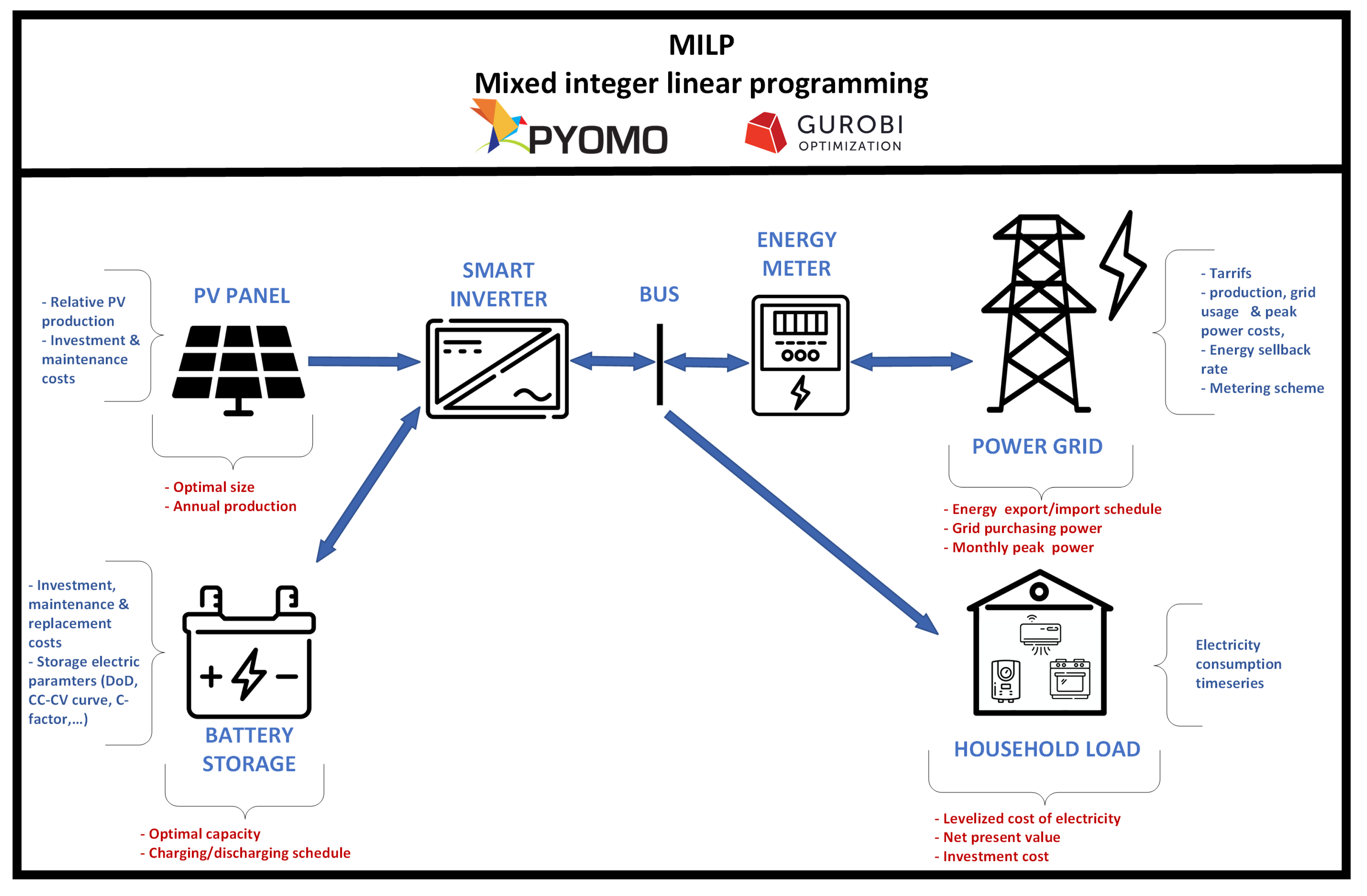
2. Mathematical Model

This section presents a deterministic optimization model for the optimal sizing and operation of a grid-tied residential PV-battery system.

Figure 1 depicts the system configuration as well as the main model input/output parameters. It is important to note that this study does not explicitly model or analyze the physical implementation or functionality of a power controller. Instead, the MILP optimization assumes idealized control, meaning that the model determines the most cost-effective operation of the PV-battery system under given constraints and input data, without considering the detailed dynamics or hardware aspects of real-time power electronics or control devices.

However, control can be achieved using smart inverters, which can manage PV curtailment and battery charging–discharging [25]. Modern smart inverters are designed with built-in communication protocols (such as Wi-Fi, Modbus, or Zigbee) that allow them to receive real-time data from smart home management units, including electricity prices, household load profiles, PV production forecasts, and optimal operation plans. The proposed optimization model can be implemented in two ways:

• The model can run on a centralized smart home management unit, which computes the optimal operation plan and sends setpoints to the smart inverter.
• Alternatively, the smart inverter’s onboard processing unit can execute the model directly if equipped with sufficient computational resources and real-time data inputs.

2.1. Objective Function

The objective function (1) minimizes the total net present cost incurred by the residential consumer, which includes investment, loan repayments, maintenance, battery replacement, and electricity costs over the project lifetime. It is calculated as the difference between the net present value of all consumers’ costs and the net present value of consumers’ profits over the considered timespan. The costs are separated into six major groups: investment costs—$C_{inv}$, loan costs—$C_{loan}^{PV}$, equipment maintenance costs—$C_{main}^{PV}$, battery replacement $C_{repl}^{BSS}$, total electric energy costs—$C_{EE}^{PV}$ and virtual costs $C_{var}$ that penalize excessive battery charging variations. End-user profits are related to profits from energy export to the grid, and they depend on electricity pricing methods as well as compensation mechanisms for excess energy exported to the grid. In the proposed model, energy is exported to the grid when there is an excess supply from either solar generation or battery discharge. Specifically, when solar production exceeds the immediate consumption needs of the household, the surplus energy is either stored in the battery or, if the battery is fully charged or surplus energy pricing is favorable, exported to the grid. Similarly, if the battery has stored energy and discharging is economically or technically favorable, any excess power beyond the household’s demand is also fed into the grid. This export mechanism plays a crucial role in optimizing energy usage, thus maximizing financial returns under different electricity pricing methods and surplus energy compensation mechanisms. In order to avoid excessive variations in battery operation that can lead to battery lifetime degradation, an additional cost $C_{var}$ that penalizes battery charging–discharging variations is introduced to the objective function.

The objective function is minimized over the set of variables $\Psi$, which can be separated into two major groups:

• Power supply investment decision variables: PV plant investment ($P_{inst}^{PV}$, $b^{PV}$), BSS; investment ($E_{cap}^{BSS}$, $b^{BSS}$), grid connection purchase power ($P^{contracted}$)
• Consumer power supply variables: PV plant production ($P_t^{PV}$), BSS operation ($P_t^{ch}$, $P_t^{ds}$, $P_{max}^{ch\_ds}$, $E_t^{BSS}$), grid supply and associated costs ($P_t^{gri{d}_{+}}$, $P_t^{gri{d}_{-}}$, $P_m^{Gmax}$).

$$\begin{array}{c}\hfill \underset{\Psi }{min}{C}_{TOTAL}^{PV}=C_{inv}+C_{loan}^{PV}+C_{main}^{PV}+C_{repl}^{BSS}+C_{EE}^{PV}+C_{var}\end{array}$$

(1)

2.2. Investment and Loan Costs

Total investment costs are calculated using Equation (2). These include the cost of the residential PV plant, battery storage, and the cost of grid connection. The fraction financed by the loan (f) is subtracted from the investment costs and is included in the objective function separately ($C_{loan}^{PV}$), so the optimal battery capacity can be easily calculated for different ratios of upfront to loan costs.

$$\begin{array}{cc}\hfill C_{inv}& =\left(c^{PV}·P_{inst}^{PV}+c^{BSS}·E_{cap}^{BSS}+c^{conn}·P^{contracted}\right)·(1-f)\hfill \end{array}$$

(2)

Annuities are calculated using (3), depending on the loan interest rate (k) and payback period (L). The present value of loan annuities (4) is calculated by discounting each annual loan annuity to its value at the present time using an appropriate discount rate and summing up their values.

$$\begin{array}{cc}\hfill C_{annuities}& ={\displaystyle \frac{\left(c^{PV}·P_{inst}^{PV}+c^{BSS}·E_{cap}^{BSS}+c^{conn}·P^{contracted}\right)·f·k}{1-{\left(1+k\right)}^{-L}}}\hfill \end{array}$$

(3)

$$\begin{array}{cc}\hfill C_{loan}^{PV}& =\sum _{y\in L}{\displaystyle \frac{C_{annuities}}{{\left(1+d\right)}^y}}\hfill \end{array}$$

(4)

2.3. Maintenance and Replacement Costs

Maintenance costs are calculated separately for the PV plant and the battery storage system (BSS) based on different cost drivers. The maintenance cost for the PV plant (5) is determined as a function of its installed capacity, reflecting the proportional increase in maintenance expenses with larger system sizes. Similarly, the maintenance cost for the battery storage system (6) is computed based on its energy storage capacity, accounting for factors such as battery degradation, replacement, and operational upkeep. These individual cost components are combined in Equation (7), which calculates their present value to obtain the total maintenance cost over the project’s lifespan. This approach ensures a comprehensive estimation of long-term maintenance expenses while considering the time value of money.

$$\begin{array}{cc}\hfill C_{main}^{PVs}& =c^{PV}·P_{inst}^{PV}·M^{PV}\hfill \end{array}$$

(5)

$$\begin{array}{cc}\hfill C_{main}^{BSS}& =c^{BSS}·E_{cap}^{BSS}·M^{BSS}\hfill \end{array}$$

(6)

$$\begin{array}{cc}\hfill C_{main}^{PV}& =\sum _{y\in Y}{\displaystyle \frac{C_{main}^{PVs}+C_{main}^{BSS}}{{\left(1+d\right)}^n}}\hfill \end{array}$$

(7)

The lifespan of a home battery storage system is influenced by several key factors, such as the number of charge–discharge cycles, typical depth of discharge, average temperature conditions, battery usage patterns, etc. The battery lifetime is usually shorter than the PV plant lifetime, necessitating periodic replacements throughout the project’s duration. To account for this, the cost of battery replacement is incorporated into the objective function to ensure an accurate assessment of the total system costs. Equation (8) calculates the discounted cost of replacing the battery at year z, considering the time value of money.

$$\begin{array}{cc}\hfill C_{repl}^{BSS}& ={\displaystyle \frac{c_{repl}^{BSS}·E_{cap}^{BSS}}{{\left(1+d\right)}^z}}\hfill \end{array}$$

(8)

Yearly energy and peak power costs (9) are determined by summing the monthly expenses for both energy consumption ($C_m^{EE}$) and peak power demand ($c^{peak}·$). The peak power cost component accounts for charges based on the maximum power drawn from the grid during a billing period. However, if the residential consumer is not subject to monthly peak power charges, the value of $c^{peak}$ should be set to zero, effectively removing this cost from the calculation.

2.4. Energy Costs and Profits

To accurately reflect the total energy and grid usage costs in the objective function, their present value is computed using Equation (10). This calculation incorporates the discount rate (d) to account for the time value of money and the energy cost growth rate (r) to consider anticipated increases in electricity prices over the project’s lifespan. By discounting future costs to their present value, the model ensures a more precise estimation of the long-term financial impact of energy consumption and peak demand charges.

$$\begin{array}{cc}\hfill C^{EE}& =\sum _{m\in M}{C}_m^{EE}+\sum _{m\in M}{c}^{peak}·P_m^{Gmax}\hfill \end{array}$$

(9)

$$\begin{array}{cc}\hfill C_{EE}^{PV}& =\sum _{y\in Y}{\displaystyle \frac{C^{EE}·{(1+r)}^y}{{(1+d)}^y}}\hfill \end{array}$$

(10)

Maximum grid power for each month must not exceed contracted capacity, which is ensured using Equation (11). Equation (12) defines total grid power in each time instance as a difference between exported and imported power from the grid. Equation (13) calculates the monthly grid peak power for month m as the maximum grid power during all periods t belonging to month m.

$$\begin{array}{cccc}\hfill P_m^{Gmax}& \le P^{contracted}\hfill & \hfill & \forall m\in M\hfill \end{array}$$

(11)

$$\begin{array}{cccc}\hfill P_t^{grid}& =P_t^{gri{d}_{+}}-P_t^{gri{d}_{-}}\hfill & \hfill & \forall t\in T\hfill \end{array}$$

(12)

$$\begin{array}{cccc}\hfill P_m^{Gmax}& \ge P_t^{gri{d}_{+}}+P_t^{grid-}\hfill & \hfill & \forall m\in M,t\in T^m\hfill \end{array}$$

(13)

Two distinct metering approaches are compared in this paper:

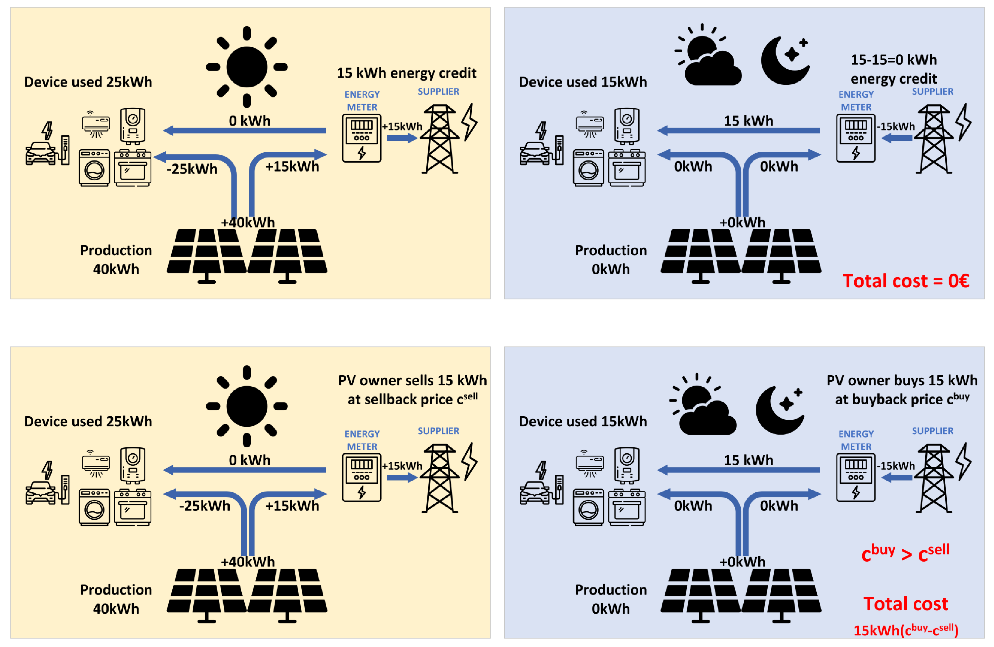
• Monthly net metering/billing: Under a pure monthly net metering compensation mechanism, any excess electricity produced by a PV system that is delivered to the grid is credited at the same retail rate that the customer would pay for electricity consumption. This means that for every kilowatt-hour (kWh) exported, the consumer receives a full kWh credit that can offset future electricity consumption from the grid. In Croatia, suppliers use a less common approach that combines both net metering and net billing simultaneously. Consumers receive full retail credits (net metering) for the portion of exported electricity equal to the amount of monthly imported electricity, but after this threshold is reached, any further excess energy is compensated at the lower rate (currently 80% of the energy retail rate [26]).
• 15 min interval net billing: Under the 15 min net billing compensation mechanism, excess electricity exported to the grid is compensated at a lower rate, rather than the full retail price. The customer is then billed separately for the electricity consumed from the grid at the standard retail rate. This often results in lower financial benefits compared to monthly net metering.

Figure 2 illustrates the concepts of net metering and net billing that are currently in place in Croatia. Under the monthly scheme, any energy surplus (15 kWh in this scenario) exported to the grid can be consumed during the same billing period (month), resulting in a total cost of zero. On the other hand, if the 15 min scheme is applied to the same scenario, the same energy surplus (15 kWh) will be exported and sold at the price $c^{sell}=c^{E.sur}·c^{E_H}$. During periods where PV production is not enough to satisfy the residential load, the prosumer has to buy (import) energy from the grid at the price $c^{buy}=(c^{Gri{d}_H}+c^{E_H}+c^{RES})·(1+VAT)$, resulting in a total scenario cost equal to 15 kWh $·((1-c^{E.sur}/(1+VAT)·c^{E_H}+c^{Gri{d}_H}+c^{RES})$. The same billing principle is applied to the dynamic energy pricing scheme, only that the energy production price $c^{E_H}$ is not constant but is dynamically changing ($c_t^E$) according to the day-ahead market price.

Equations (14)–(21) are used to calculate monthly net energy exchange with the power grid under the monthly net metering/billing scheme. Net energy at high and low tariffs for each month is calculated from the total energy imported and exported to the grid for that month. For each tariff, there can either be a deficit or surplus of energy at the end of the month. Binary variables $b_m^{HT}$ and $b_m^{LT}$ ensure that there can not be both a deficit and a surplus of energy for any given month. Therefore, from Equations (15) and (19), the net energy for each month at high and low tariffs will be equal to either a monthly energy deficit or a negative monthly energy surplus.

$$\begin{array}{cccc}\hfill E_m^{HT}& =\sum _{t\in C^{m^{HT}}}{P}_t^{grid}·\Delta t\hfill & \hfill & \forall m\in M\hfill \end{array}$$

(14)

$$\begin{array}{cccc}\hfill E_m^{HT}& =E_m^{HTimp}-E_m^{HTexp}\hfill & \hfill & \forall m\in M\hfill \end{array}$$

(15)

$$\begin{array}{cccc}\hfill 0\le E_m^{HTimp}& \le b_m^{HT}·L^{annual}\hfill & \hfill & \forall m\in M\hfill \end{array}$$

(16)

$$\begin{array}{cccc}\hfill 0\le E_m^{HTexp}& \le (1-b_m^{HT})·L^{annual}\hfill & \hfill & \forall m\in M\hfill \end{array}$$

(17)

$$\begin{array}{cccc}\hfill E_m^{LT}& =\sum _{t\in C^{m^{LT}}}{P}_t^{grid}·\Delta t\hfill & \hfill & \forall m\in M\hfill \end{array}$$

(18)

$$\begin{array}{cccc}\hfill E_m^{LT}& =E_m^{LTimp}-E_m^{LTexp}\hfill & \hfill & \forall m\in M\hfill \end{array}$$

(19)

$$\begin{array}{cccc}\hfill 0\le E_m^{LTimp}& \le b_m^{LT}·L^{annual}\hfill & \hfill & \forall m\in M\hfill \end{array}$$

(20)

$$\begin{array}{cccc}\hfill 0\le E_m^{LTexp}& \le (1-b_m^{LT})·L^{annual}\hfill & \hfill & \forall m\in M\hfill \end{array}$$

(21)

Equations (22)–(25) are used to calculate the total energy imports and exports for high and low tariffs under the 15 min interval net metering/billing scheme. Under this scheme, there can be both a deficit and surplus of energy for each month since these are calculated for each time instance separately. If there is energy being imported from the grid for any given period, it will be added to the total energy imported from the grid for that month with Equation (22) or (24), depending on the tariff. The same applies to the exported energy.

$$\begin{array}{cccc}\hfill E_m^{HTimp}& =\sum _{t\in C^{m^{HT}}}{P}_t^{gri{d}_{+}}·\Delta t\hfill & \hfill & \forall m\in M\hfill \end{array}$$

(22)

$$\begin{array}{cccc}\hfill E_m^{HTexp}& =\sum _{t\in C^{m^{HT}}}{P}_t^{gri{d}_{-}}·\Delta t\hfill & \hfill & \forall m\in M\hfill \end{array}$$

(23)

$$\begin{array}{cccc}\hfill E_m^{LTimp}& =\sum _{t\in C^{m^{LT}}}{P}_t^{gri{d}_{+}}·\Delta t\hfill & \hfill & \forall m\in M\hfill \end{array}$$

(24)

$$\begin{array}{cccc}\hfill E_m^{LTexp}& =\sum _{t\in C^{m^{LT}}}{P}_t^{gri{d}_{-}}·\Delta t\hfill & \hfill & \forall m\in M\hfill \end{array}$$

(25)

where $C^{m^{HT}}$ and $C^{m^{LT}}$ are sets of time instances in month m with high or low energy tariffs.

The monthly energy bill for both metering schemes can be calculated using Equation (26) with {$E_m^{HTimp},E_m^{HTexp},E_m^{LTimp},E_m^{LTexp}$}, defined with (15)–(19) for monthly net metering/billing, and (22)–(25) for 15 min net billing.

Under the monthly net metering/billing scheme, if there is a surplus of energy generated by the PV system for a given month, $E_m^{HTimp}$ will be equal to zero; hence, the high tariff energy bill will be negative. Surplus energy in high tariff, $E_m^{HTexp}$, will be sold at a price equal to energy production costs in high tariff $c^{E_H}$ multiplied by energy surplus price to energy production price ratio $c^{E.sur}$. A value of $c^{E.sur}\le 1$ indicates that the price of sold energy is lower than the price of purchased energy. Grid usage costs are not included in the selling price. Since a high tariff is valid during most of the sunshine hours, there cannot be a surplus of energy in a low tariff. The second part of the equation will be greater than zero in most cases. For a month with surplus energy in a high tariff, if the profit from sold energy is greater than the energy cost in a low tariff, the monthly energy bill will be negative, lowering the total energy cost calculated using Equation (10).

Under the 15 min interval net metering/billing scheme, for any given month, both $E_m^{HTexp}$ and $E_m^{HTimp}$ can be greater than 0. If there is an energy surplus during any period t in the considered month m, it will be sold at a price equal to $c^{E.sur}·c^{E_H}$, which is considerably lower than the purchasing price ($(c^{Gri{d}_H}+c^{E_H}+c^{RES})·(1+VAT)$. This scenario is unfavorable for prosumers compared to the monthly net metering/billing scheme.

$$\begin{array}{cc}\hfill C_m^{EE}=& (c^{Gri{d}_H}+c^{E_H}+c^{RES})·(1+VAT)·E_m^{HTimp}\hfill \\ & +(c^{Gri{d}_L}+c^{E_L}+c^{RES})·(1+VAT)·E_m^{LTimp}\hfill \\ & -c^{E.sur}·c^{E_H}·E_m^{HTexp}-c^{E.sur}·c^{E_L}·E_m^{LTexp},\forall m\in M\hfill \end{array}$$

(26)

Although the model assumes two different time-of-use (ToU) electricity price periods, it can be easily generalized to integrate more complex ToU pricing structures. By adjusting the optimization framework, additional tariff segments or dynamic pricing schemes can be incorporated without significant modifications to the core methodology. This flexibility allows the model to adapt to various regulatory environments and market conditions, making it applicable to a wide range of real-world energy pricing scenarios.

Special sub-case under the 15 min interval net metering/billing scheme is considered when energy prices $c^{E_H}$ and $c^{E_L}$ are not fixed but instead are varying dynamically, in line with day-ahead market prices. Modifying Equation (26) is required to calculate the monthly electricity bill under dynamic energy pricing:

$$\begin{array}{c}\hfill \begin{array}{cc}\hfill C_m^{EE}=& (c^{Gri{d}_H}+c^{RES})·(1+VAT)·E_m^{HTimp}+(c^{Gri{d}_L}+c^{RES})·(1+VAT)·E_m^{LTimp}\hfill \\ \hfill & +(1+VAT)·C_m^{imp}+C_m^{exp},\forall m\in M\hfill \end{array}\end{array}$$

(27)

In the dynamic pricing model, grid usage costs can still be defined through ToU tariffs and can be calculated separately for two different periods of the day (HT and LT). Additional Equations (28) and (29) calculate the monthly cost for energy exported to and imported from the grid, where $c_t^E$ is the dynamic energy price at period t.

$$\begin{array}{cccc}\hfill C_m^{imp}& =\sum _{t\in C^m}{P}_t^{gri{d}_{+}}·c_t^E\hfill & \hfill & \forall m\in M\hfill \end{array}$$

(28)

$$\begin{array}{cccc}\hfill C_m^{exp}& =\sum _{t\in C^m}{P}_t^{gri{d}_{-}}·c_t^E·c^{E.sur}\hfill & \hfill & \forall m\in M\hfill \end{array}$$

(29)

2.5. Battery Storage and PV Plant Operation

Optimal PV power is determined using Equation (30), where $b^{PV}$ is the solar plant binary decision variable. Equation (31) ensures that PV production for each period is limited to PV plant capacity while allowing for PV power curtailment.

$$\begin{array}{cc}\hfill 0& \le P_{inst}^{PV}\le P_{inst}^{PV.max}·b^{PV}\hfill \end{array}$$

(30)

$$\begin{array}{cccc}\hfill P_t^{PV}& \le P_t^{PV.pu}·P_{inst}^{PV}·{\eta }_{inv}\hfill & \hfill & \forall t\in T\hfill \end{array}$$

(31)

The next set of equations ensures normal battery operation. Battery state of charge (SoC) at the end of any period t depends on initial SOC and charging–discharging power during previous periods (Equations (32) and (33)) and is limited to battery capacity (Equations (34) and (35)). Maximum charging–discharging power is calculated from battery capacity and its C factor (36). For a battery of 4 kWh capacity with a C factor equal to 2, the maximum charging–discharging power would be 2 kW. Constraint (37) limits discharging power $P_t^{ds}$ during all time periods to maximum charge–discharge power. The maximum charging power $P_{max,t}^{ch}$ for the given period t is determined by battery SOC. Equation (40) is used to determine $P_{max,t}^{ch}$ from the battery CC-CV curve. The linear relationship between charging power and the battery’s state of charge is expressed using the approach described in [27]. Constraint (38) limits the charging power $P_t^{ch}$ to $P_{max,t}^{ch}$ calculated for each period t.

$$\begin{array}{cc}\hfill E_1^{BSS}& =E_{init}^{BSS}+\left(P_1^{ch}·{\eta }_{ch}-{\displaystyle \frac{P_1^{ds}}{{\eta }_{ds}}}\right)\Delta t\hfill \end{array}$$

(32)

$$\begin{array}{cccc}\hfill E_t^{BSS}& =E_{t-1}^{BSS}+\left(P_t^{ch}·{\eta }_{ch}-{\displaystyle \frac{P_t^{ds}}{{\eta }_{ds}}}\right)\Delta t\hfill & \hfill & \forall t\in T\hfill \end{array}$$

(33)

$$\begin{array}{cc}\hfill 0& \le E_{cap}^{BSS}\le E_{cap}^{BSS.max}·b^{BSS}\hfill \end{array}$$

(34)

$$\begin{array}{cccc}\hfill DoD& ·E_{cap}^{BSS}\le E_t^{BSS}\le E_{cap}^{BSS}\hfill & \hfill & \forall t\in T\hfill \end{array}$$

(35)

$$\begin{array}{cc}\hfill P_{max}^{ch\_ds}& ={\displaystyle \frac{E_{cap}^{BSS}}{C^{BSS}}}\hfill \end{array}$$

(36)

$$\begin{array}{cccc}\hfill 0& \le P_t^{ds}\le P_{max}^{ch\_ds}\hfill & \hfill & \forall t\in T\hfill \end{array}$$

(37)

$$\begin{array}{cccc}\hfill 0& \le P_t^{ch}\le P_{max,t}^{ch}\hfill & \hfill & \forall t\in T\hfill \end{array}$$

(38)

$$\begin{array}{cccc}\hfill P_{max,t}^{ch}& \le P_{max}^{ch\_ds}\hfill & \hfill & \forall t\in T\hfill \end{array}$$

(39)

$$\begin{array}{cccc}\hfill P_{max,t}^{ch}& \le {\displaystyle \frac{E_{cap}^{BSS}-E_t^{BSS}}{C^{BSS}-C^{BSS}·r_{limit}^{CC-CV}}}\hfill & \hfill & \forall t\in T\hfill \end{array}$$

(40)

The application of time-of-use (ToU) tariffs and net metering can introduce additional variations in battery operation, as different charging and discharging patterns may yield the same objective function value. This occurs when energy import and export prices remain constant over extended time spans, allowing multiple operational strategies to achieve similar cost (objective function) outcomes. Consequently, the model must balance cost optimization with operational smoothness, preventing excessive battery cycling that could lead to efficiency losses and increased battery degradation. Given this, abrupt changes in battery charging–discharging power are penalized so that a more realistic charging profile is obtained by the model. Change in battery power charging–discharging is defined as the difference between charging powers in two sequential time periods (Equations (43) and (44)). Equation (41) sums all charging–discharging changes for each year, while (42) converts annual penalties into a present value that is included in the objective function. The penalization factor is carefully chosen to minimize its impact on the objective function value while effectively reducing oscillations in battery operation.

$$\begin{array}{cc}\hfill C_{var}^{annual}& =\sum _{t\in T}{P}_t^{ch.ramp}\hfill \end{array}$$

(41)

$$\begin{array}{cc}\hfill C_{var}& =\sum _{y\in Y}{\displaystyle \frac{pen·C_{var}^{annual}}{{(1+d)}^y}}\hfill \end{array}$$

(42)

Equations (43) and (44) are used to determine variations in charging–discharging to be penalized in Equation (42).

$$\begin{array}{cccc}\hfill \left|P_t^{ch}-P_{t-1}^{ch}\right|& \le P_t^{ch.ramp}\hfill & \hfill & \forall t=2,\dots ,T\hfill \end{array}$$

(43)

$$\begin{array}{cccc}\hfill \left|P_t^{ds}-P_{t-1}^{ds}\right|& \le P_t^{ch.ramp}\hfill & \hfill & \forall t=2,\dots ,T\hfill \end{array}$$

(44)

Finally, the power balance (Equation (45)) is achieved by equaling the power drawn from the grid, PV system, or battery with the power used to satisfy load demand and/or charge the battery.

$$\begin{array}{cccc}\hfill P_t^{grid}+P_t^{PV}+P_t^{ds}& =P_t^{ch}+L_t\hfill & \hfill & \forall t\in T\hfill \end{array}$$

(45)

The optimization model described earlier was implemented in Pyomo [28], with a Gurobi solver [29] used to solve the problem. The simulation ran on a server equipped with an AMD Ryzen 7 1700 processor (3 GHz) and 16 GB of RAM.

3. Case Study

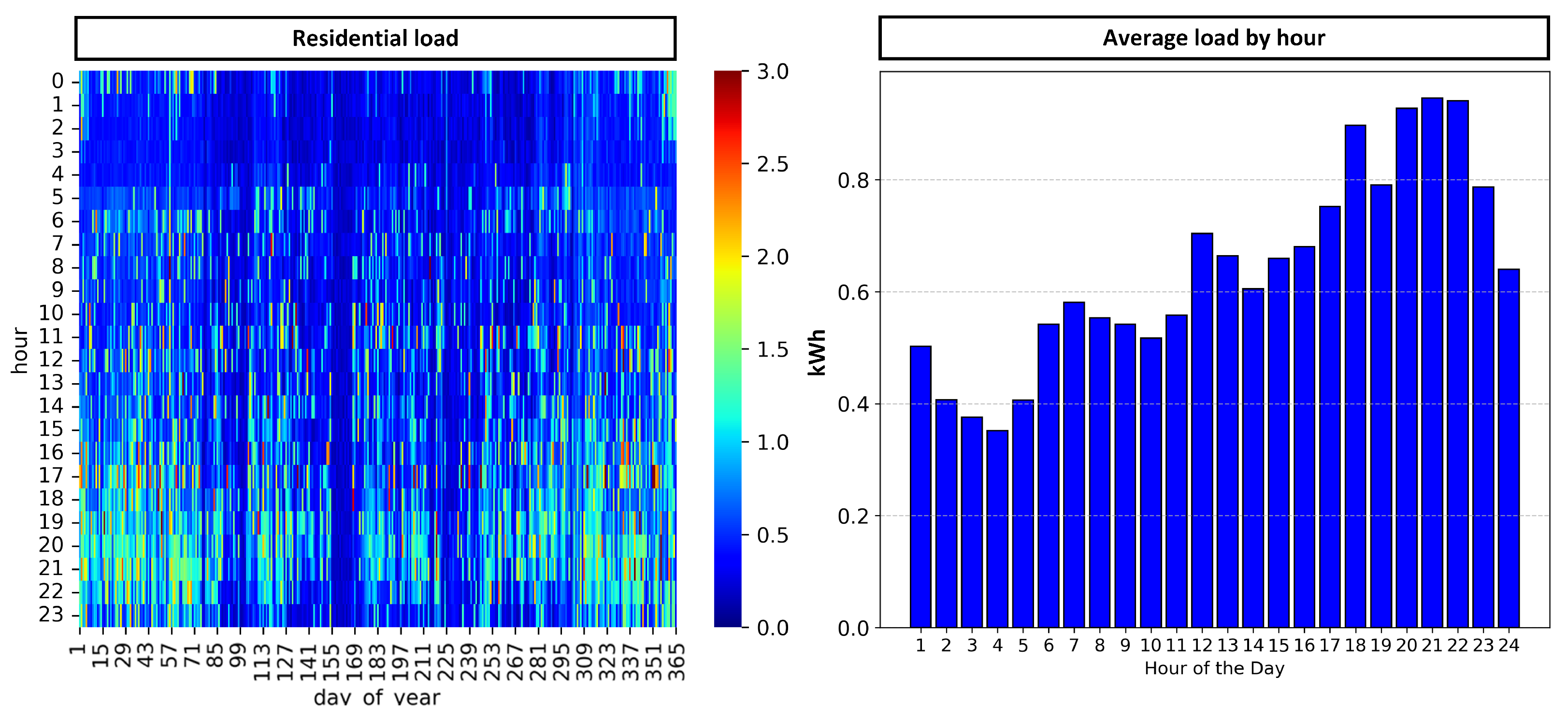
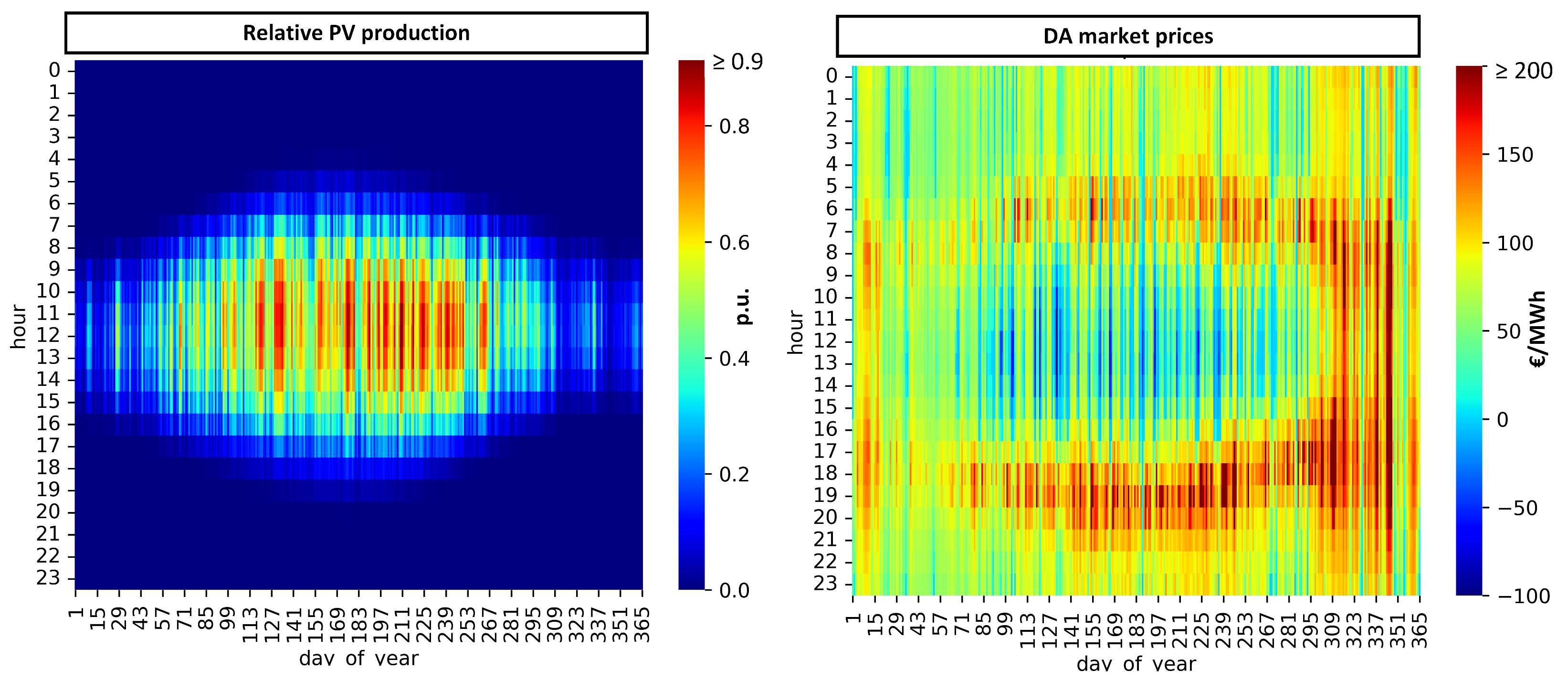
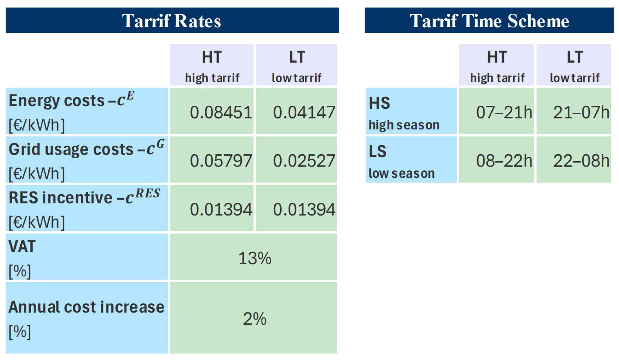
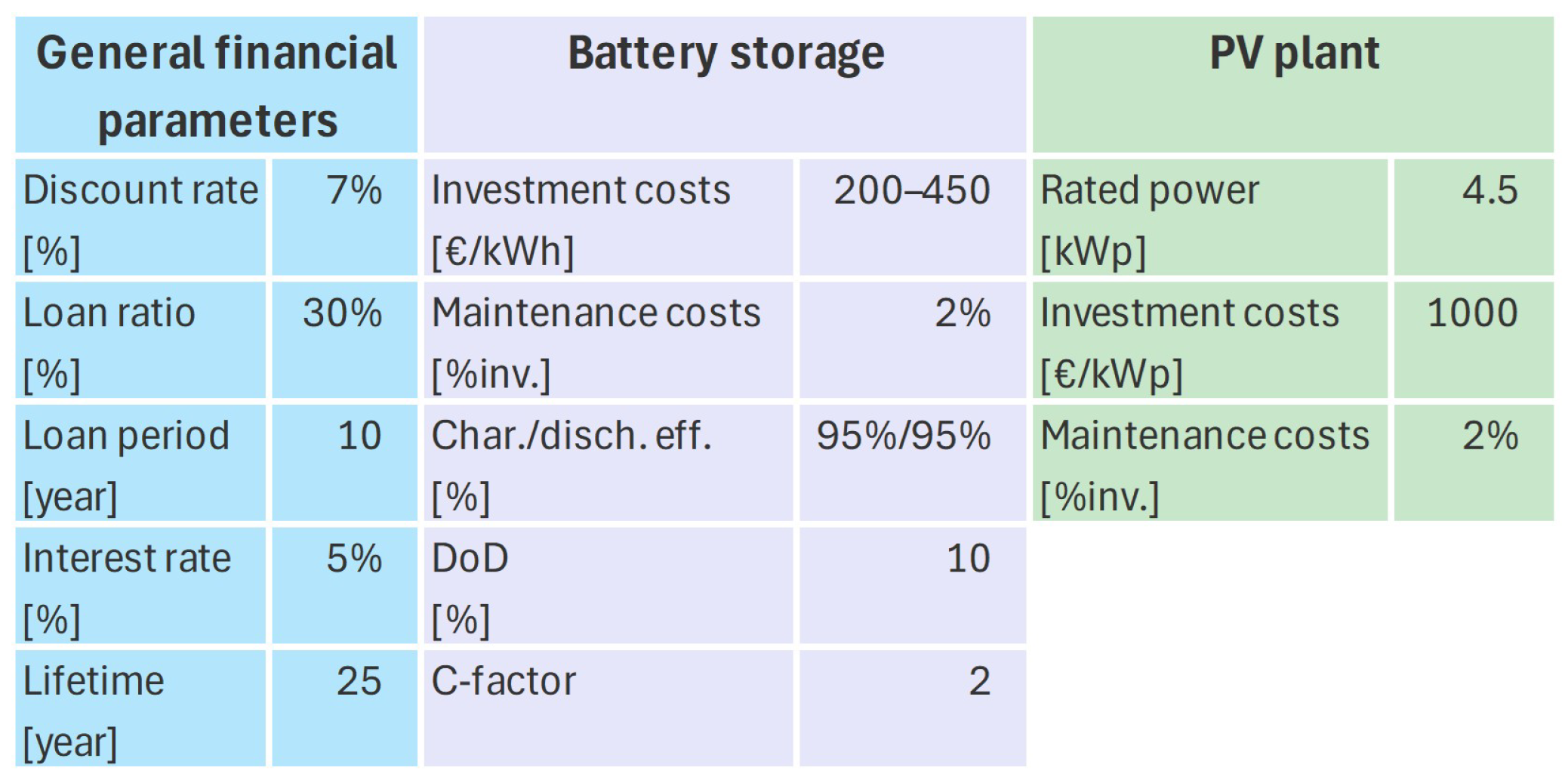
3.1. Input Data Description

The optimization model was applied to a single residential household with an approximate annual energy consumption of ≈5600 kWh. While the full optimization model allows for the simultaneous optimization of both PV plant and battery storage capacities, for this particular test case, the PV installation capacity was set at 4.5 kWp, resulting in an estimated annual energy generation of approximately ≈5500 kWh. Figure 3 shows a heatmap of the residential electricity load profile and a bar plot of the average hourly load. Although the load pattern is largely stochastic, there is a noticeable increase in electricity consumption during the early evening hours, which coincides with the beginning of the low-tariff period. From the PV production and price heatmaps in Figure 4, periods of high PV production coinciding with low electricity prices are evident.

Most households in Croatia employ a two-tariff system for electricity pricing, commonly known as the “White” tariff model [30], which offers different rates based on the time of day, as detailed in Figure 6. This ToU tariff is designed to encourage more efficient energy use and balance grid load. The high tariff (HT), also called the “day” or “peak” rate, applies during periods of higher electricity demand (typically from 7:00 a.m. to 9:00 p.m.) while the low tariff (LT), also known as the “night” or “off-peak” rate, is in effect during periods of lower electricity demand (usually from 9:00 p.m. to 7:00 a.m.). The price difference between high and low tariffs is substantial, with HT rates typically ≈2 times higher than LT rates. In the dynamic pricing model, only certain components of the tariff costs are considered. Specifically, the costs associated with grid usage and renewable energy incentives are included, while traditional ToU energy costs are replaced with dynamic day-ahead (DA) market prices.

A comparison between government-regulated ToU prices and DA market prices is shown in Figure 5. Average market prices are obviously higher than ToU prices, reaching almost ten times higher values during the high-price period in December.

The ToU prices shown in Figure 5 and Figure 6 are valid for residential consumers, while business users pay 50% higher energy costs, and grid usage costs remain equal for both types of users.

Other input data and assumptions relevant to the analysis are provided in Figure 7. The case study included a comprehensive analysis of the economic viability of battery storage systems for residential PV installations. It explored a wide range of parameters to identify the critical thresholds and optimal configurations for battery storage investments. The study examined battery storage investment costs ranging from 200 to 450 EUR/kWh. This broad range allows for a detailed assessment of how varying investment costs impact the economic feasibility of battery storage systems.

An additional key aspect of the study was the investigation of the influence of solar excess energy remuneration mechanisms and energy sellback rates on optimal battery storage sizing. In the analysis, energy sellback rates were considered in the range from 0 (no profit from energy sellback) to 1 (surplus energy sold at the same price as the buyback price). By systematically exploring these variables, the study sheds light on the intricate dynamics between PV energy remuneration methods, sellback pricing, and the battery storage costs on the optimal sizing of battery systems for residential PV installations.

3.2. Numerical Results and Discussion

The optimization model described in Section 2 was used to determine the optimal battery storage size as well as the optimal system operation for residential grid-connected PV systems. Depending on the electricity pricing scheme as well as the excess solar energy remuneration mechanism, three different test cases were considered:

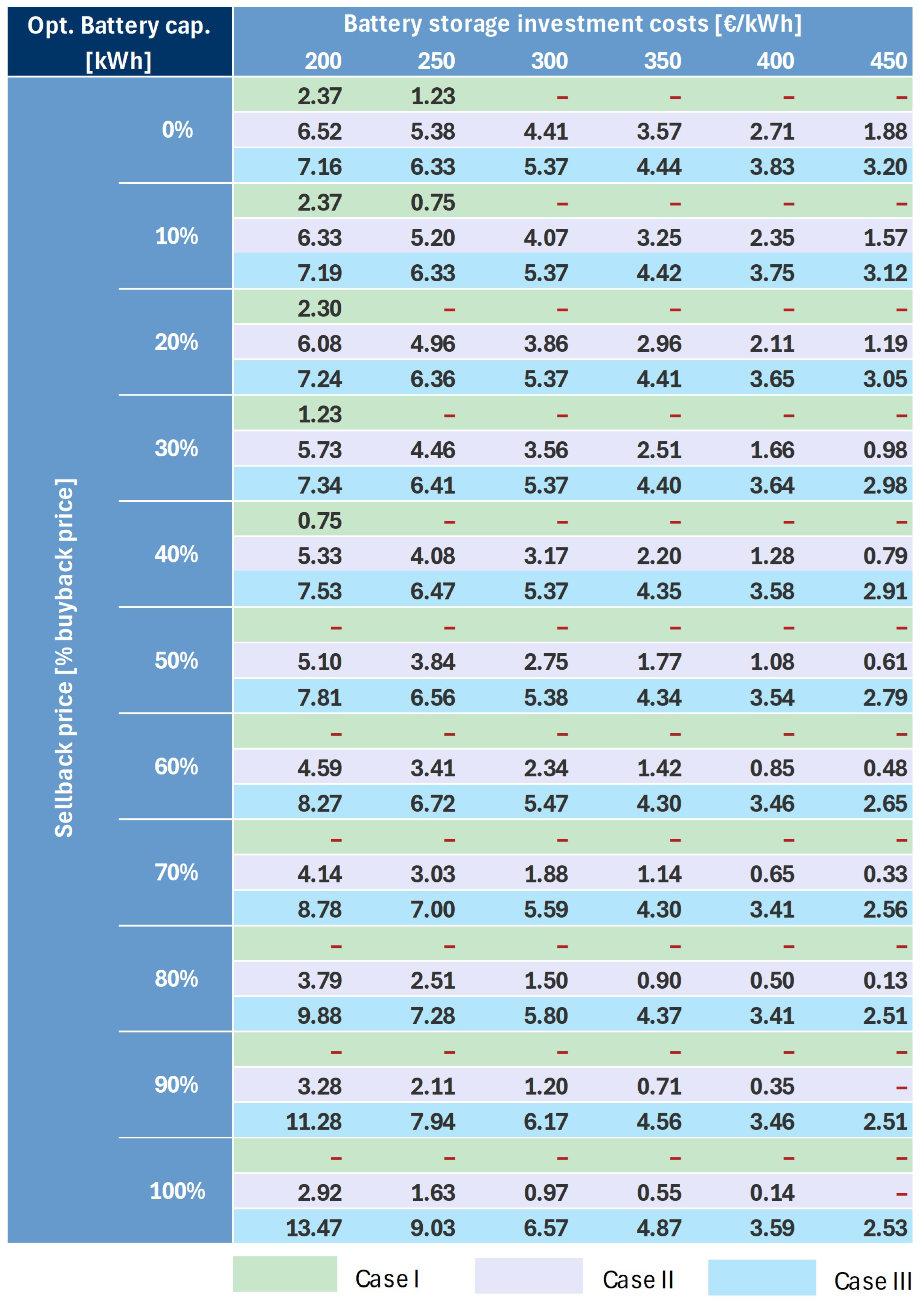
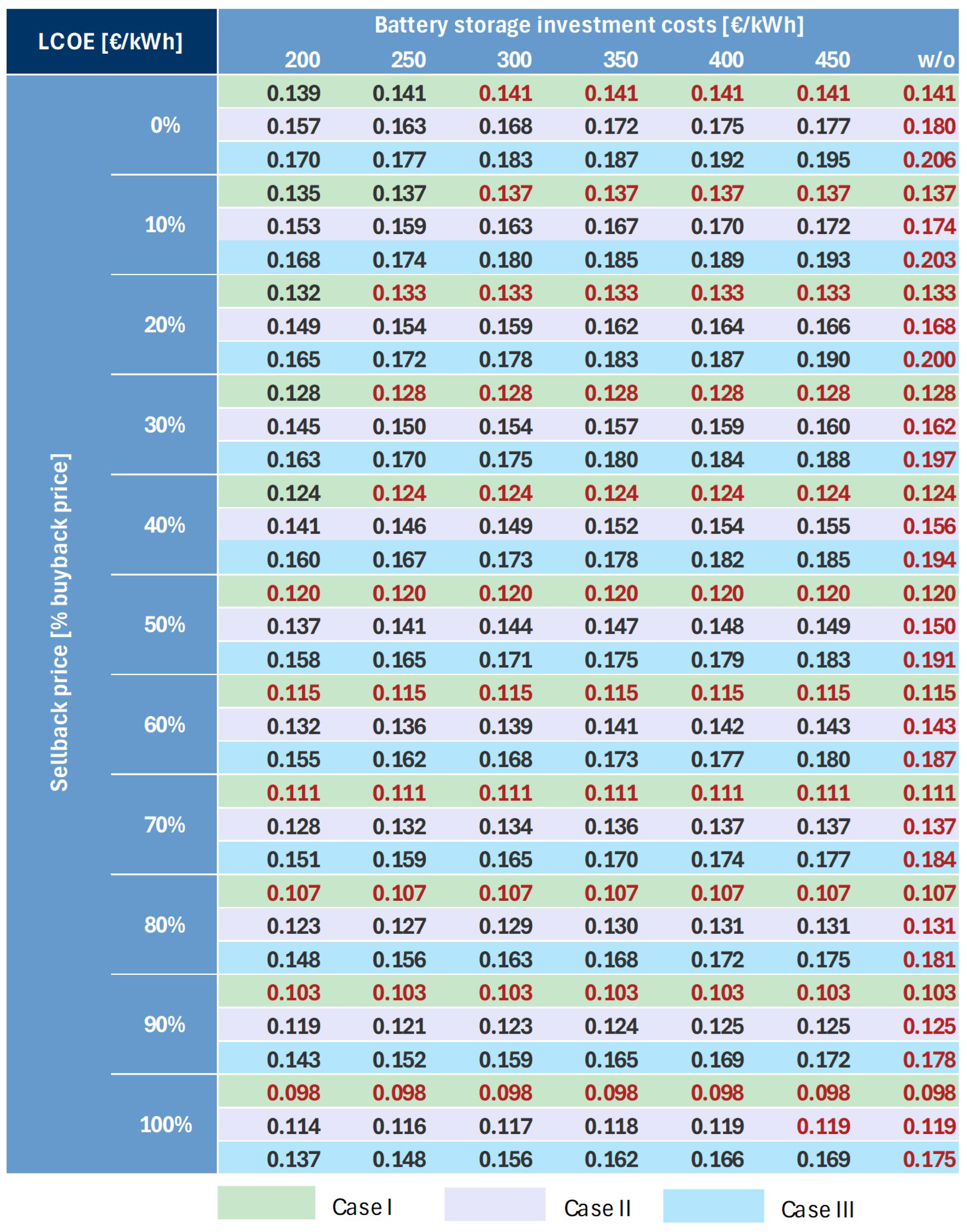
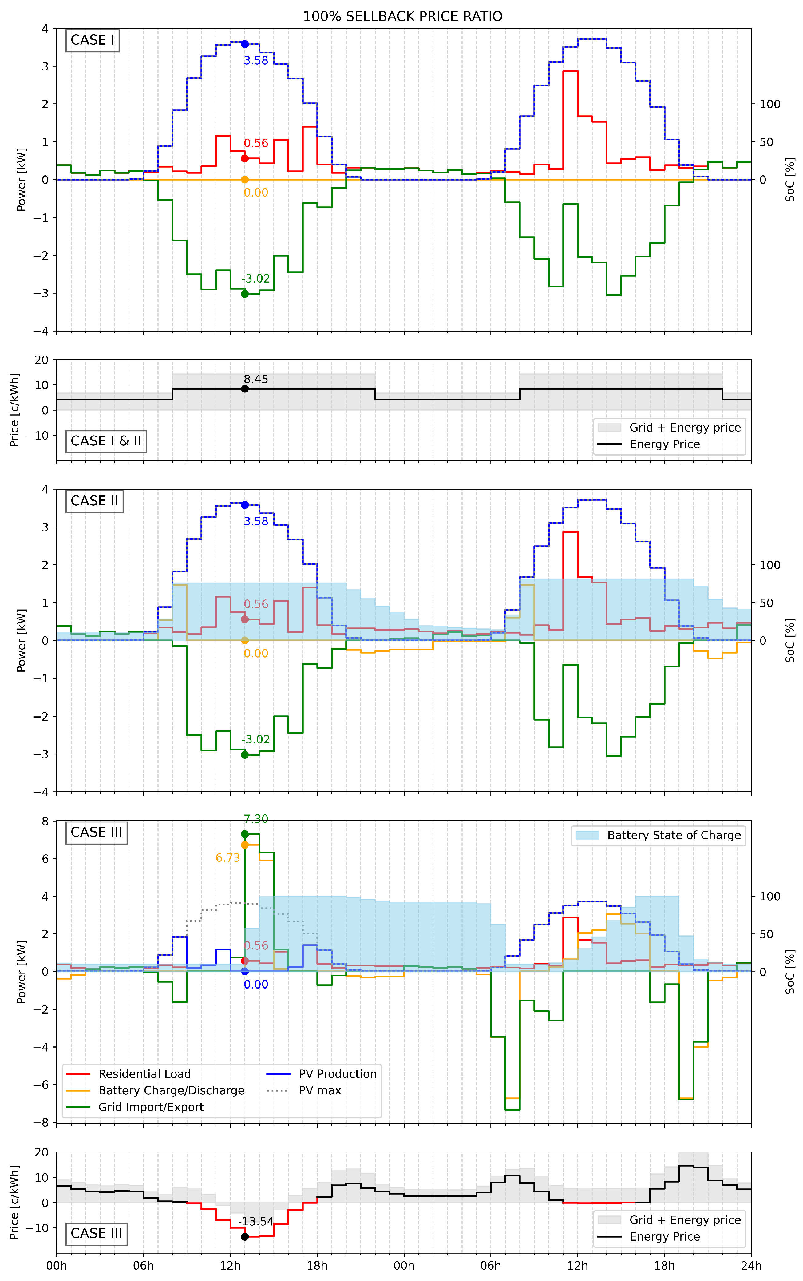
• CASE I—involves a monthly net metering/billing scheme with ToU tariff prices that is currently used in most residential grid-connected PV systems in Croatia;
• CASE II—involves a 15 min net billing scheme with ToU tariff prices that is usually used for industrial grid-connected PV prosumers in Croatia;
• CASE III—involves a 15 min net billing scheme with dynamic day-ahead market prices.

Dynamic electricity pricing is expected to be introduced within the next few years [31], with increased electricity production from RES. Negative prices during periods with high RES production will stimulate consumers to increase electricity consumption and therefore help balance the power system. From the prosumers’ standpoint, dynamic pricing offers a chance for extra profit with smart consumption and production scheduling.

The energy export sellback price in all three cases is expected to be lower or equal to the import energy price. By scaling the energy surplus price to the energy production price ratio (sellback price ratio) $c^{E.sur}$ from 0% to 100%, the impact of different sellback prices on optimal battery storage size can be observed. Battery storage investment cost is crucial when determining its optimal size. Prices of BSS per kWh are currently in decline and are expected to be even lower within a few years. To investigate the influence of BSS prices, calculations were performed with BSS prices ranging from 200 to 450 EUR/kWh [32]. Battery replacement was predicted at a fraction of the original cost, taking into consideration declining prices. Due to improvements to battery technology, only one replacement was predicted for the entire lifetime of the project.

The optimal battery capacity for different solar energy sellback prices and battery investment costs across various electricity pricing/solar remuneration schemes is given in Figure 8. In the case of monthly net metering/billing (CASE I), investing in BSS is only viable if the sellback price ratio $c^{E.sur}$ is rather low. Since most of the energy produced by the PV system is consumed during the same month, only a small amount of surplus energy is sold at the end of the month. For a sellback price greater than 40% of the buyback price, investing in BSS would only increase the net present cost. Storing energy to be used in periods with high consumption in CASE I reduces NPC only for low BSS cost (250 EUR/kWh or less) and $c^{E.sur}\le 40\%$.

Switching to a 15 min net metering/billing scheme changes the situation significantly. Any produced energy not consumed within a 15 min period is sold at a much lower price than the price of energy purchased from the grid. That is true even if $c^{E.sur}=100\%$ since the sellback price in Croatia does not include grid costs, VAT, or RES support tax. Optimal BSS capacity increases with a decreasing value of $c^{E.sur}$ in CASE II, reaching a maximum value of 6.52 kWh for $c^{E.sur}=0\%$ and a BSS price of 200 EUR/kWh. At BSS price of 450 EUR/kWh and $c^{E.sur}\ge 90\%$, investing in BSS is not economically viable.

The introduction of dynamic prices completely changes the operation of the residential PV plant. In the traditional time-of-use (ToU) model (CASE II) using 15 min net billing, prosumers typically benefit from exporting surplus energy during high-tariff periods, resulting in economic gains. However, the dynamic pricing model introduces a new dimension of variability and risk. Power systems with a high percentage of solar energy can experience negative prices during periods of peak PV production coinciding with low system load. This operating scenario presents a significant challenge for prosumers because exporting energy during negative price periods could result in economic losses if the relative sellback price ($c^{E.sur}$) is greater than 0%. This situation forces prosumers to consider alternative strategies for managing surplus energy. When faced with negative market prices, prosumers have two primary options:

• Limiting the output of the PV system to avoid exporting energy at a loss;
• Utilizing BSS to store surplus energy for later use or sale when market conditions are more favorable.

As the relative sellback price ($c^{E.sur}$) increases in CASE III, the optimal BSS capacity also tends to increase. This relationship is driven by several factors:

• Energy purchased at negative/low prices can be stored and later sold during peak price periods, creating an arbitrage opportunity. With the increase in the relative sellback price ($c^{E.sur}$), the profit from arbitrage opportunity increases.
• A larger BSS capacity allows for greater energy manipulation, potentially increasing income through strategic buying and selling.
• The ability to store more energy provides a buffer against price volatility on a daily basis and enhances system flexibility to handle/market PV production surplus.

Despite the potential for energy arbitrage, the net present cost (NPC) in CASE III remains higher than that in CASE I or II for the same combinations of relative sellback price ($c^{E.sur}$) and BSS investment costs (as shown in Figure 9). This outcome can be attributed to the following factors:

• The average DA market prices are higher than the current regulated ToU tariff prices in Croatia;
• The analysis assumes that the consumer load pattern remains unchanged under the dynamic pricing tariff, similar to the load pattern observed under the ToU tariff.

The NPC decrease achieved with BSS investment is shown in the last column in Figure 9. Only small savings can be achieved in CASE I, where the NPC is 1.7% smaller for $c^{E.sur}=0\%$ and a BSS price of 200 EUR/kWh compared to the NPC of an option that does not include a BSS. Larger savings can be achieved in CASE II (up to 13%). The maximum possible savings decrease with the increase in $c^{E.sur}$ for both CASE I and II. Investing in a BSS offers larger economic gains in CASE III, where a comparatively high battery capacity of 13.47 kWh can result in a decrease of 22% in the NPC for $c^{E.sur}=100\%$. Unlike CASES I and II, possible savings increase with the increase in $c^{E.sur}$.

Current regulated electricity prices in Croatia, calculated including all the costs shown in Figure 6, are 0.176 EUR/kWh (high tariff) and 0.090 EUR/kWh (low tariff). For a residential consumer with the load profile same as used in this paper, the average import price is equal to 0.145 EUR/kWh, calculated with 36.1% LT and 63.9% HT consumption. Without a PV plant, and assuming that the same load profile is kept for the next 25 years, the levelized cost of electricity calculated with a 2% annual price increase and 7% discount rate is equal to 0.175 EUR/kWh for ToU tariff prices and 0.194 EUR/kWh for dynamic prices. With the residential PV plant installed, the LCOE calculated for the entire project lifetime of 25 years is shown in Figure 10. The results show that even with dynamic DA prices that represent a significant increase over current regulated prices, prosumers can achieve lower LCOE (0.137–0.170 EUR/kWh) assuming a BSS price of 200 EUR/kWh. For higher BSS prices, CASE III LCOE values start to exceed 0.175 EUR/kWh. When $c^{E.sur}$ increases, LCOE values for all three cases follow the same pattern as NPC values, as expected.

Additional sensitivity analyses were conducted to evaluate the impact of potential multiple battery replacements (2–4 replacements over the 25-year project lifetime). The results show that a second replacement increases the NPC by ≤2.2% and reduces optimal battery capacity by ≤1.1 kWh in CASE III, across the whole range of battery investment prices and sellback prices. The maximum NPC increase and optimal capacity decrease occur for the battery price of 200 EUR/kWh and 100% sellback price. Since the optimal battery capacity, specifically, in CASE III, is generally lower for higher battery prices and lower sellback prices, the influence of a second replacement on the NPC is very low in those cases.

Replacement costs are discounted to the present value (Equation (8)), resulting in a second replacement near the end of the project’s lifetime, contributing minimally to the NPC due to the relatively high value of the originally assumed 7% discount rate. Reducing the discount rate to 4% amplifies the impact of additional battery replacement on the NPC increase, resulting in a maximum NPC increase of 4.8%.

More frequent replacements (3–4) further reduce profitability (up to 9.55% higher NPC) but remain unlikely given that results show optimal system operation with one battery charge–discharge cycle per day (Figure 11). Such use of batteries aligns with typical lithium-ion battery lifespan assumptions of around 10 years under moderate cycling.

Figure 11 shows the differences in the optimal operation of residential PV systems with optimal BSS capacity for a selected 2-day period in all three cases for a low sellback price ratio equal to $c^{E.sur}=10\%$. This particular 2-day period is of interest because of the lowest negative price on the DA market of the entire year that occurs during the first of the selected 2 days.

During the first day, PV production exceeds residential consumption by a large margin. In CASE I and II, most surplus energy from the PV system is exported to the grid, while a smaller part of surplus energy is used to charge the battery. The main difference between CASE I and CASE II is the optimal BSS capacity, 2.37 vs. 6.33 kWh, respectively. Therefore, the energy stored in the battery is sufficient to cover the load during night hours in CASE II, while additional energy has to be purchased from the grid in CASE I.

In CASE I, the implementation of monthly net metering and billing plays a pivotal role in determining the financial benefits for the consumer. While the relative sellback price may appear low, this remuneration method offers considerable savings due to the unique way in which it credits the consumer.

Specifically, for every kilowatt-hour (kWh) of energy exported to the grid, the consumer receives a full kWh credit, which can then be used to offset their future electricity consumption. This means that, even with a lower sellback price, the consumer benefits from an effective means of reducing their overall energy costs by using their excess energy to cover future electricity needs.

Furthermore, in CASE I, the relative sellback price is only applied to the energy exported to the grid that exceeds the monthly energy import. This ensures that consumers are not penalized for exporting the energy they need for their own consumption, which further enhances the cost-effectiveness of the system. Given these considerations, low-capacity BSS proves to be the optimal solution. A low-capacity BSS is mainly used to enable the usage of excess PV plant production under a low tariff. This is especially relevant in Croatia, where net metering is applied separately to each tariff, and energy credits can only be used within the specific tariff they were earned.

CASE III exhibits an entirely different optimal operation. Energy is purchased from the grid during periods with the most negative prices (13:00–15:00 on day 1). Most of the energy produced by the PV plant is curtailed since charging the battery with negatively priced energy from the grid generates profit for the end consumer and lowers the monthly electricity bill (Equations (27) and (28)), while charging the battery with PV energy does not. The peak charging power is much higher in CASE III since most of the charging coincides with the most negative prices, while the charging power in CASE I and II does not fluctuate significantly. The energy stored in BSS is later exported to the grid during periods with the highest prices.

During the 2nd day of the selected period, negative energy prices do occur, but the total import price (that includes grid costs) stays positive. Therefore, there is no battery charging from the grid on the 2nd day, and during this day, the battery is charged only using surplus production from the PV plant. During the 2nd day, energy is exported to the grid through BSS discharge in the morning and early evening periods, which correlate with high positive prices on the DA market. Additionally, in these periods, excess PV production is also exported to the grid, generating profit from surplus production.

The optimal operation for the same 2-day period with a sellback price ratio of $c^{E.sur}=100\%$ is shown in Figure 12. The optimal solution for CASE I does not include battery storage; any surplus energy is exported to the grid. Battery capacity in CASE II with $c^{E.sur}=100\%$ (2.92 kWh) is reduced compared to $c^{E.sur}=10\%$ (6.33 kWh). This results in more energy exported to the grid during sunshine hours and some energy imported during night hours because the smaller battery capacity is insufficient to cover the load during the night.

With the increased sellback price ratio, CASE III follows the same operation pattern (energy import during negative prices and export during highest prices), but peak grid and charging power have almost doubled. The economic gain from BSS participating in arbitrage through optimal energy charge–discharge is much higher, with increased $c^{E.sur}$ causing much higher optimal battery capacity (13.47 kWh) and grid/charging power.

4. Conclusions

Investing in residential battery storage offers financial benefits to households by reducing electricity bills through strategic energy usage, providing backup power during outages, and potentially increasing property value, while also leveraging government incentives and tax credits to offset initial investment costs. The optimal sizing of battery storage in residential PV systems is a complex task considering different net metering/billing mechanisms, excess PV energy sellback rates, electricity pricing policies, and varying investment costs into the battery system. This study presents a comprehensive mixed-integer linear programming framework for optimal sizing and operation of residential battery storage in grid-connected PV systems, with a focus on the Croatian electricity system and its unique pricing mechanisms. The analysis explicitly considers Croatia’s hybrid net metering/net billing schemes, time-of-use (ToU) tariffs, and dynamic pricing, as well as the impact of battery investment costs and compensation rates for excess PV energy. While the proposed model is flexible and can be readily adapted to billing schemes in other countries, such a comparative analysis is beyond the scope of this paper and could be a subject of future research.

The results show that, under the current Croatian monthly net metering/billing scheme, the financial benefits of residential battery storage are limited—even when excess energy sellback rates are low. In contrast, the 15 min net billing scheme, especially when combined with ToU tariffs or dynamic pricing, offers greater potential for household savings, provided that battery investment costs continue to decline.

However, these benefits are highly sensitive to the structure of electricity tariffs and the spread between retail and feed-in prices, as also observed in recent European studies [7,14,18]. Our findings reinforce that well-designed policies and targeted incentives are essential to maximize the value of battery storage for Croatian households, particularly as the market evolves toward more dynamic and granular pricing.

The results indicate that optimal battery capacity differs considerably between various price situations, emphasizing the importance of considering both technical and economic factors in optimizing battery storage systems, particularly in the context of an evolving regulatory framework. Future research should focus on integrating more sophisticated forecasting models and exploring policy incentives to enhance the economic feasibility of residential battery storage systems.

References

1. Zhang, N.; Leibowicz, B.D.; Hanasusanto, G.A. Optimal Residential Battery Storage Operations Using Robust Data-Driven Dynamic Programming. IEEE Trans. Smart Grid 2020, 11, 1771–1780. [Google Scholar] [CrossRef]
2. Mohamed, A.A.R.; Best, R.J.; Liu, X.; Morrow, D.J. Residential Battery Energy Storage Sizing and Profitability in the Presence of PV and EV. In Proceedings of the 2021 IEEE Madrid PowerTech, Madrid, Spain, 28 June–2 July 2021; pp. 1–6. [Google Scholar] [CrossRef]
3. World Bank. Economic Analysis of Battery Energy Storage Systems; Technical Report; World Bank: Washington, DC, USA, 2020. [Google Scholar]
4. Nottrott, A.; Kleissl, J.; Washom, B. Energy dispatch schedule optimization and cost benefit analysis for grid-connected, photovoltaic-battery storage systems. Renew. Energy 2013, 55, 230–240. [Google Scholar] [CrossRef]
5. Guidara, I.; Tina, G.M.; Souissi, A.; Chaabene, M. Techno-economic adequacy for PV-Battery sizing of a residential grid-connected installation. In Proceedings of the 2020 11th International Renewable Energy Congress (IREC), Hammamet, Tunisia, 29–31 October 2020; pp. 1–5. [Google Scholar] [CrossRef]
6. Shabani, M.; Dahlquist, E.; Wallin, F.; Yan, J. Techno-economic impacts of battery performance models and control strategies on optimal design of a grid-connected PV system. Energy Convers. Manag. 2021, 245, 114617. [Google Scholar] [CrossRef]
7. Pan, X.; Khezri, R.; Mahmoudi, A.; Muyeen, S. Optimal planning of solar PV and battery storage with energy management systems for Time-of-Use and flat electricity tariffs. IET Renew. Power Gener. 2022, 16, 1206–1219. [Google Scholar] [CrossRef]
8. Li, J. Optimal sizing of grid-connected photovoltaic battery systems for residential houses in Australia. Renew. Energy 2019, 136, 1245–1254. [Google Scholar] [CrossRef]
9. Akram, U.; Khalid, M.; Shafiq, S. Optimal sizing of a wind/solar/battery hybrid grid-connected microgrid system. IET Renew. Power Gener. 2018, 12, 72–80. [Google Scholar] [CrossRef]
10. Khalilpour, R.; Vassallo, A. Planning and operation scheduling of PV-battery systems: A novel methodology. Renew. Sustain. Energy Rev. 2016, 53, 194–208. [Google Scholar] [CrossRef]
11. Gitizadeh, M.; Fakharzadegan, H. Battery capacity determination with respect to optimized energy dispatch schedule in grid-connected photovoltaic (PV) systems. Energy 2014, 65, 665–674. [Google Scholar] [CrossRef]
12. Ru, Y.; Kleissl, J.; Martinez, S. Storage Size Determination for Grid-Connected Photovoltaic Systems. IEEE Trans. Sustain. Energy 2013, 4, 68–81. [Google Scholar] [CrossRef]
13. Aghamohamadi, M.; Mahmoudi, A.; Haque, M.H. Two-Stage Robust Sizing and Operation Co-Optimization for Residential PV–Battery Systems Considering the Uncertainty of PV Generation and Load. IEEE Trans. Ind. Inform. 2021, 17, 1005–1017. [Google Scholar] [CrossRef]
14. Zhou, L.; Zhang, Y.; Lin, X.; Li, C.; Cai, Z.; Yang, P. Optimal Sizing of PV and BESS for a Smart Household Considering Different Price Mechanisms. IEEE Access 2018, 6, 41050–41059. [Google Scholar] [CrossRef]
15. Yen, M.Y.C.; Tan, W.S.; Ng, W.L.; Wu, Y.K. Solar and Battery Sizing for Maximum Savings Implementation in Malaysia’s Buildings. In Proceedings of the 2021 IEEE International Future Energy Electronics Conference (IFEEC), Taipei, Taiwan, 16–19 November 2021; pp. 1–6. [Google Scholar] [CrossRef]
16. Chang, H.; Jing, F.L.; Hou, Y.L.; Chen, L.Q.; Yang, Y.J.; Liu, T.Y.; Wei, C.L.; Zhai, B.Q.; Hou, C.Y. Development of a Mathematical Model to Size the Photovoltaic and Storage Battery Based on the Energy Demand Pattern of the House. Front. Energy Res. 2022, 10, 945180. [Google Scholar] [CrossRef]
17. Parray, M.T.; Martinsen, T. Multi-year analysis for optimal behind-the-meter battery storage sizing and scheduling: A Norwegian case study. J. Energy Storage 2025, 110, 115304. [Google Scholar] [CrossRef]
18. Hiesl, A.; Ramsebner, J.; Haas, R. Economic viability of decentralised battery storage systems for single-family buildings up to cross-building utilisation. Smart Energy 2024, 16, 100160. [Google Scholar] [CrossRef]
19. Bucciarelli, L.L. The effect of day-to-day correlation in solar radiation on the probability of loss-of-power in a stand-alone photovoltaic energy system. Solar Energy 1986, 36, 11–14. [Google Scholar] [CrossRef]
20. Bucciarelli, L.L. Estimating loss-of-power probabilities of stand-alone photovoltaic solar energy systems. Solar Energy 1984, 32, 205–209. [Google Scholar] [CrossRef]
21. Ofry, E.; Braunstein, A. The loss of power supply probability as a technique for designing stand-alone solar electrical (photovoltaic) systems. IEEE Trans. Power Appar. Syst. 1983, 5, 1171–1175. [Google Scholar] [CrossRef]
22. Egido, M.; Lorenzo, E. The sizing of stand alone PV-system: A review and a proposed new method. Sol. Energy Mater. Sol. Cells 1992, 26, 51–69. [Google Scholar] [CrossRef]
23. Hafiz, F.; Lubkeman, D.; Husain, I.; Fajri, P. Energy Storage Management Strategy Based on Dynamic Programming and Optimal Sizing of PV Panel-Storage Capacity for a Residential System. In Proceedings of the 2018 IEEE/PES Transmission and Distribution Conference and Exposition (T&D), Denver, CO, USA, 16–19 April 2018; pp. 1–9. [Google Scholar] [CrossRef]
24. Mahmood, M.; Chowdhury, P.; Yeassin, R.; Hasan, M.; Ahmad, T.; Chowdhury, N.U.R. Impacts of digitalization on smart grids, renewable energy, and demand response: An updated review of current applications. Energy Convers. Manag. X 2024, 24, 100790. [Google Scholar] [CrossRef]
25. Balogun, O.A.; Sun, Y.; Gbadega, P.A. Coordination of smart inverter-enabled distributed energy resources for optimal PV-BESS integration and voltage stability in modern power distribution networks: A systematic review and bibliometric analysis. e-Prime Adv. Electr. Eng. Electron. Energy 2024, 10, 100800. [Google Scholar] [CrossRef]
26. Clean Energy for EU Islands Secretariat. Net Metering and Net Billing in Croatia: What It Means for the Promotion of RES Electricity. 2025. Available online: https://clean-energy-islands.ec.europa.eu/ (accessed on 20 February 2025).
27. Vagropoulos, S.I.; Bakirtzis, A.G. Optimal Bidding Strategy for Electric Vehicle Aggregators in Electricity Markets. IEEE Trans. Power Syst. 2013, 28, 4031–4041. [Google Scholar] [CrossRef]
28. Hart, W.E.; Watson, J.P.; Woodruff, D.L. Pyomo: Modeling and solving mathematical programs in Python. Math. Program. Comput. 2011, 3, 219–260. [Google Scholar] [CrossRef]
29. Gurobi Optimization, LLC. Gurobi Optimizer Reference Manual. Gurobi Optimization, LLC. 2024. Available online: https://docs.gurobi.com/projects/optimizer/en/current/index.html (accessed on 15 January 2025).
30. HEP Operator Distribucijskog Sustava d.o.o. (HEP ODS). Tariff Rates (Prices) for Households. 2025. Available online: https://www.hep.hr/ods/korisnici/kucanstvo/tarifne-stavke-cijene/160# (accessed on 19 February 2025).
31. Croatian Energy Regulatory Agency (HERA). Annual Report for 2022. 2023. Available online: https://www.hera.hr/en/html/annual_reports.html (accessed on 18 February 2025).
32. Cole, W.; Karmakar, A. Cost Projections for Utility-Scale Battery Storage: 2023 Update; National Renewable Energy Lab. (NREL): Golden, CO, USA, 2023. [Google Scholar]
Figure 1. System configuration with model parameters.
Energies 18 02391 g001
Figure 2. Illustration of monthly (top) and 15 min (bottom) net metering/billing scheme.
Energies 18 02391 g002
Figure 3. Heatmap of the residential electricity load profile (left) and the bar plot of the average hourly load (right).
Energies 18 02391 g003
Figure 4. Heatmap of the relative PV production and DA market prices used in the dynamic pricing model.
Energies 18 02391 g004
Figure 5. Energy cost ( c E ) comparison for June and December 2024.
Energies 18 02391 g005
Figure 6. Overview of time-of-use tariff rates.
Energies 18 02391 g006
Figure 7. Model input data.
Energies 18 02391 g007
Figure 8. Optimal battery storage capacity for different sellback ratios and BSS investment costs.
Energies 18 02391 g008
Figure 9. The net present cost (NPC) for different sellback ratios and BSS investment costs.
Energies 18 02391 g009
Figure 10. Levelized cost of electricity for different sellback ratios and BSS investment costs.
Energies 18 02391 g010
Figure 11. Optimized residential power supply: A 2-day operation comparison for different test cases at a 10% relative sellback rate.
Energies 18 02391 g011
Figure 12. Optimized residential power supply: A 2-day operation comparison for different test cases at a 100% relative sellback rate.
Energies 18 02391 g012
Disclaimer/Publisher’s Note: The statements, opinions and data contained in all publications are solely those of the individual author(s) and contributor(s) and not of MDPI and/or the editor(s). MDPI and/or the editor(s) disclaim responsibility for any injury to people or property resulting from any ideas, methods, instructions or products referred to in the content.