Article

Comparing Fast Fourier Transform and Prony Method for Analysing Frequency Oscillation in Real Power System Interconnection

by
Didik Fauzi Dakhlan
1,2,*,
Joko Muslim
2,3,
Indra Kurniawan
2,
Kevin Marojahan Banjar-Nahor
1,
Bambang Anggoro Soedjarno
1 and
Nanang Hariyanto
1
1
School of Electrical Engineering and Informatics, Bandung Institute of Technology, Bandung 40132, Indonesia
2
PT PLN (Persero), Jakarta 12160, Indonesia
3
Institut Teknologi (IT) PLN, Jakarta 11750, Indonesia
*
Author to whom correspondence should be addressed.
Energies 2025, 18(9), 2377; https://doi.org/10.3390/en18092377
Submission received: 30 March 2025 / Revised: 23 April 2025 / Accepted: 1 May 2025 / Published: 6 May 2025
(This article belongs to the Topic Modern Power Systems and Units)

Abstract

:
Analysing power system oscillations is essential for maintaining electrical grid stability and reliability. To assess power system oscillations and demonstrate the actual application in a real grid system, this research compares two popular signal processing methods: Prony’s approach and the Fast Fourier Transform from Phasor Measurement Unit data in the Java Bali (Indonesia) power system interconnection. FFT gives information about the prominent frequency components by representing system oscillations in the frequency domain. Nevertheless, windowing effects and resolution limitations limit it. By fitting exponential functions to time-domain signals, Prony’s approach, on the other hand, excels at precisely estimating the frequency and damping characteristics of oscillatory modes. The accuracy, computational effectiveness, and applicability for the real-time monitoring of both approaches are assessed in this study. Simulation results on both simulated and actual power system data illustrate the benefits and drawbacks of each strategy. The results show that although FFT is helpful for rapid spectral analysis, Prony’s approach offers more thorough mode identification, which makes it especially advantageous for damping evaluations. This study ends with suggestions for choosing the best method for power system stability analysis based on application requirements.

1. Introduction

The power system is a complex and dynamic network that demands continuous monitoring, control, and protection, along with prompt interventions to ensure its reliable and secure operation. Observing key parameters such as voltage, current, and frequency is crucial for detecting abnormalities and implementing necessary corrective measures. These parameters are inherently non-stationary and comprise various components, including harmonics, inter-harmonics, and transients. Detecting even minor variations in these signals at an early stage is essential for determining precise corrective actions. Therefore, the application of appropriate signal processing techniques is vital to accurately extract relevant information, facilitating swift decision-making and timely responses.
Figure 1 shows the relationship between how fast protection systems respond and how wide their coverage is in a power system. Local protection, like fast relays, works at a specific point and reacts in milliseconds to quickly clear faults. Zonal or backup protection covers a larger area, such as a substation, and responds slightly slower. PMU-based systems and WAMS offer protection over a wide area with response times of a few seconds. SCADA and EMS cover the whole network but respond more slowly, in minutes, and are mainly used for monitoring and control rather than immediate protection.
Various blackout events or widespread disturbances have occurred and have impacted millions of people on Earth. The last incident also occurred in the electric power system in Indonesia, especially in the Java Bali interconnection system on 4 August 2019. This incident was recorded as one of the blackout disturbances that had a very large impact. A blackout event or widespread disturbance is usually not a stand-alone event. Blackouts usually begin with disturbances in one of the backbone transmission segments, large generators, or large loads that suddenly disappear. There is a delay time when a blackout occurs, with the initial trigger in minutes or more than hours [1,2,3].
Previously, conventional main and backup protection schemes have been implemented to anticipate any possibilities of fault in power systems as instantaneous reactive measures followed by defense schemes; for example, automatic load shedding and frequency curtailment up to the final stage of islanding of subsystems have been set in operation as a contingency to ensure the stability of power systems and balance both generating and loading after the fault interruption whenever necessary.
This research will be devoted especially to the PMU (Phasor Measurement Unit) data analysis, which is able to give information about the power system condition more quickly than the conventional Supervisory Control and Data Acquisition (SCADA)/Energy Management System (EMS) and a more widely monitored range compared to conventional protection and control systems.
A key tool in signal processing, the Fast Fourier Transform (FFT) converts signals from the time domain to the frequency domain to analyze their frequency content. It can be challenging to interpret many real-world signals in the time domain because they comprise many frequency components, such as electrical waveforms, audio signals, and communication signals. By dissecting these signals into their constituent frequency components, FFT enables researchers and engineers to more easily spot patterns, spot anomalies, and implement filtering strategies. In power system analysis [4,5], FFT helps identify harmonics, inter-harmonics, and oscillations in voltage and current waveforms, which are crucial for maintaining system stability and power quality. FFT has many drawbacks despite its benefits. It is less useful for analyzing transitory signals since it assumes that signals are stationary inside the observation frame. Furthermore, if the signal is not periodic inside the sampling frame, spectral leakage may happen.
Since its beginnings, Prony analysis, which was first proposed by French mathematician Gaspard Riche de Prony, has been regarded as a potent tool and is used in a variety of domains, including mechanical engineering, biomedical signal analysis, control systems, and power systems [6,7,8,9,10,11,12,13,14,15,16,17,18]. This analytic technique identifies both oscillatory and exponentially decaying components within the related signal source by breaking down a signal into the sum of exponential functions. This specific technique is helpful for determining the dynamic system’s modes, spotting oscillations, and determining the stability of the system being studied.
Although the method’s origins were primarily theoretical, the development of digital computing has made it possible to apply Prony analysis in engineering and signal processing in a convenient and user-friendly manner, particularly in complex power systems. For example, it can be used to detect oscillatory modes that could cause larger system failures and to monitor the stability of large interconnections [9,10,11,12]. In fact, while processing a series of data, including a low-frequency spectrum as a field of interest, it is required to establish the matching down sampling factor (DSF) as the trade-off between computing efficiency and model correctness [19].
Small disturbance (small-signal) stability and large disturbance (transient) stability are two well-established categories of stability disturbance that are closely linked to the rotor angle stability in power system applications nowadays. Small-signal stability is vulnerable to minor disruptions and typically causes low-frequency oscillations in the power system. The power system is stable if these oscillations can be controlled in a way that keeps the system state variable deviation inside the system stability threshold for an extended period of time. Therefore, the sooner the power system’s ability to sustain synchronism in the face of even minor disruptions is evaluated, the greater the likelihood that the system will resume stable operation.
The instability may result from a constant increase in the rotor angle brought on by insufficient synchronizing torque or from an increase in the amplitude of rotor oscillations brought on by insufficient dampening torque. Inadequate damping is more closely linked to the problems of today’s power system’s with small signal stability [20,21,22,23,24,25,26,27,28,29,30]. The damping ratio threshold (ξ) to suppress the damping torque is arbitrary and depends on a number of variables, including the stiffness of the system itself, configurations, and the type of generation and control. NERC’s interconnection oscillation analysis showed ξ > 0.1 as well damped [31]; the Indonesian grid code specifies ξ ≥ 0.1 [32], and the State Grid Corporation in China uses ξ = 0.02 [33]. The typical damping ratio is defined as ξ = 0.03–0.05 [34].
Conversely, transient stability entails significant power system disruptions caused by appreciable variations in operating parameters, including voltage, current, and frequency. A phenomenon known as transient stability occurs instantly and is typically noticeable in a matter of seconds. Transmission line outages brought on by short circuits or major generator trips are the main causes of this. Blackouts will eventually result from cascading occurrences that were not foreseen by the appropriate, selective, and coordinated protection and control mechanisms [2,32,33,34,35,36,37,38,39,40].
In order to assess the efficiency, accuracy, and applicability of the FFT with Prony’s approach for power system oscillation analysis, this study was conducted. Grid stability may be impacted by power system oscillations, which necessitate careful examination to determine their frequency components and damping properties. Because of its processing efficiency, FFT is frequently used for frequency-domain analysis, which makes it appropriate for determining the prominent oscillatory components. Its ability to capture fleeting signals and resolve tightly spaced frequencies is limited, though. Prony’s method, on the other hand, is perfect for analyzing transient events and system stability since it offers a comprehensive parametric approach by calculating both frequency and damping characteristics. The purpose of this study is to assess different techniques according to several criteria including accuracy, computational effectiveness, and the capacity to examine both transient and steady-state oscillations. This study offers insights into choosing the best method for power system monitoring and stability assessments by contrasting their advantages and disadvantages.
To ensure a balanced evaluation, this study explicitly discusses the limitations and practical considerations of both the FFT and Prony methods when applied to power system oscillation analysis. The FFT is known for its computational efficiency and simplicity; however, it suffers from reduced frequency resolution and is highly sensitive to windowing effects, particularly when analyzing short-duration signals obtained from PMU measurements [4,41,42]. These limitations make FFT less effective in resolving closely spaced modes or tracking oscillations with non-stationary behavior. In contrast, the Prony method demonstrates superior capability in estimating mode frequencies and damping ratios from time-domain data, especially for low-frequency oscillations where FFT resolution may be insufficient. Moreover, the practical application of each method has been discussed in the context of real-world system monitoring, such as in the Java-Bali 500 kV interconnection. Considerations regarding computational complexity and suitability for real-time implementation have also been included, highlighting the trade-offs between estimation accuracy and operational feasibility in wide-area monitoring systems.

2. Materials and Method

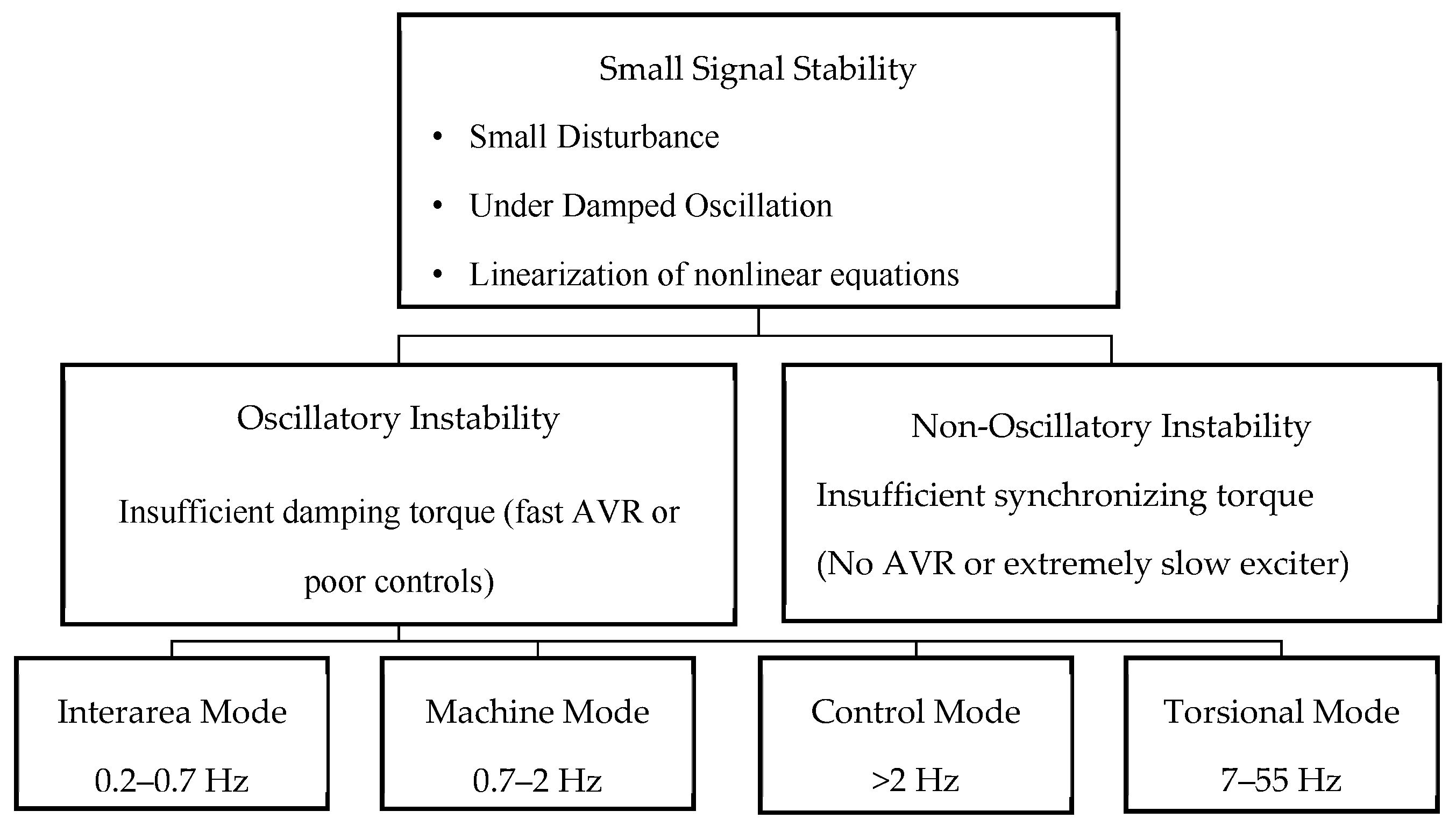
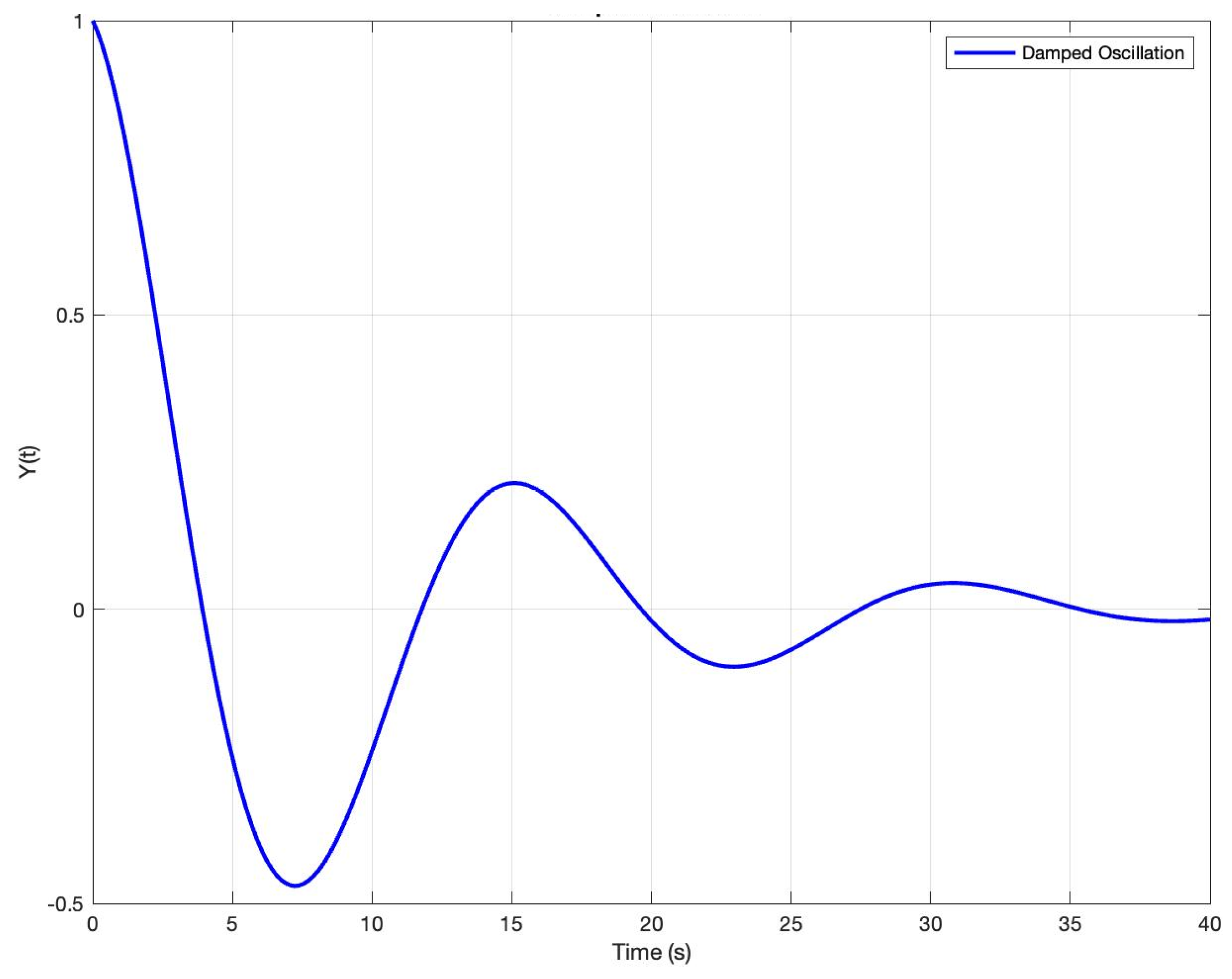
2.1. Small-Signal Stability

The power system’s ability to stay in sync at all times during and after minor disruptions is known as small-signal stability or the stability of small disturbances. Small variations in loads or generators, or a short circuit tripping of the tie line, might cause minor disruptions [30,31,32,33,34]. Figure 2 shows the classification of small signal stability. Small-signal instability, also known as non-oscillatory instability, is characterized by an increase in the rotor angle that is primarily brought on by insufficient synchronizing torque. The rotor’s higher amplitude oscillation, which results from inadequate damping torque, is known as oscillatory instability.
Interarea oscillations correspond to electro-mechanical oscillations between two parts of an electric power system [43]. Usually seen in large power networks with weak tie lines, they can also have an impact on smaller systems if two generating locations are joined by a relatively weak line. When generators on one side of the connection line begin to oscillate against generators on the other side, periodic electric power transfer occurs down this line (along with side effects on the rest of the system). These oscillations have frequencies between 0.2 and 2.0 Hz. These oscillations can cause instability in some situations, but they will be absorbed in a matter of seconds in well-damped systems.
Figure 2. Small signal stability classification [44].
Energies 18 02377 g002

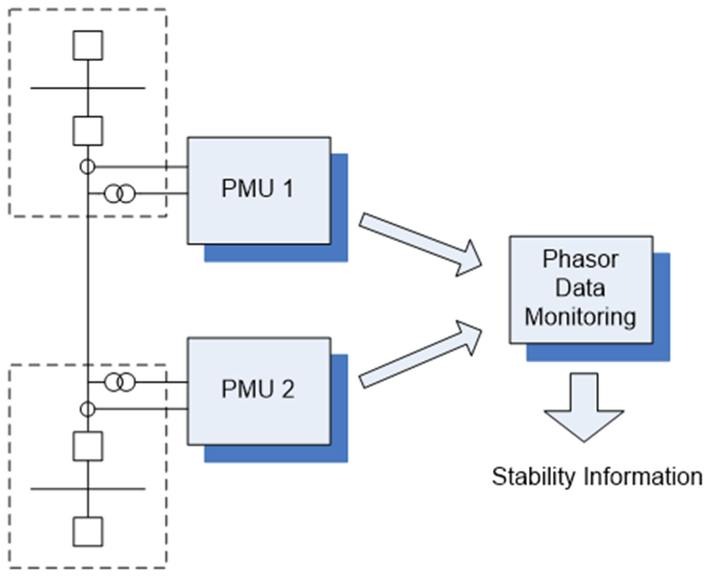
2.2. Phasor Measurement Unit

A Phasor Measurement Unit (PMU) is defined by IEEE as a device or a function in a multifunction device that produces synchronized phasor, frequency, and rate of change of frequency (ROCOF) estimates from voltage and/or current signals and a time synchronizing signal [45]. The PMU is expected to measure the exact electrical waveforms from a grid with reference to the Coordinated Universal Time (UTC) by the Global Positioning System (GPS).
Figure 3 shows the PMU configuration used in this work. PMUs shall provide exact replica measurements of voltage and current synchro phasors and are scaled by a constant factor of the actual primary high voltage and current. The use of instrumentation transformers, i.e., Potential Transformers (PTs) or Capacitive Voltage Transformers (CVTs) and Current Transformers (CTs); connecting control cables and connected burdens; and analog-to-digital converters may introduce certain levels of errors, including the GPS equipment characteristic and system asymmetries [39]. Compliance with IEEE Std C37.118.1 [45] requirements shall enable the PMUs to deliver the overall accuracy and put them into acceptable operational function.
Due to time constraints of data collection and computation time, decisions based on PMU data are not suitable for very rapid actions. However, the PMU is ideal for wider-area protection systems where the PMU will indicate system stability conditions due to low-frequency oscillations. However, with the development of the data-driven concept for system stability, signal processing is not too long. Thus, mitigation, action, and contingency plans can be immediately known and implemented. The PMU will receive input from the primary measurement data of the electric power system in the form of equipment status (open/close), voltage from the Voltage Transformer (VT) and current from the Current Transformer (CT). These data will be synchronized with the GPS and then sent to the Phasor Data Concentrator (PDC) to be processed into the required information. This phasor data will be sampled according to the setting (usually per 1 or 2 cycles) sent continuously.

2.3. Fast Fourier Transform

A popular method for examining power system oscillations [4,5] is the Fast Fourier Transform (FFT), which transforms time-domain signals into frequency-domain data. Determining the frequency components of oscillations that power systems frequently suffer as a result of faults, switching activities, or disturbances is essential for evaluating system stability. These oscillating signals can be broken down into their sinusoidal components using FFT, which allows for the detection of dominant frequencies, harmonics, and inter-harmonics. Resonance condition diagnosis, power system stabilizer (PSS) tuning, and overall grid dependability are all aided by these data. FFT does have certain drawbacks, though, namely its dependence on window length, spectrum leakage, and the challenge of precisely determining damping factors [4,41,42]. Because of its computing efficiency, FFT is nevertheless a vital tool for power system monitoring and stability analysis in spite of these limitations. Mathematically, the Discrete Fourier Transform (DFT), which FFT efficiently computes, is given as
X k = n = 0 N 1 x ( n ) e j 2 π k n / N ,   k = 0,1 , 2 , , N 1
where
  • X(k) represents the frequency-domain components;
  • x(n) is the time-domain signal;
  • N is the total number of samples;
  • k denotes the frequency index;
  • e j 2 π k n / N represents the complex exponential basis function.
The FFT algorithm significantly reduces the computational complexity of the DFT from O(N) to O(N log N), making it practical for real-time power system analysis. By applying FFT, power engineers can quickly assess oscillation frequencies, identify instability risks, and implement necessary control measures to maintain grid stability.

2.4. Prony Method

The fastest synchro phasor estimator is the well-known one-cycle Fourier filter, which only requires a one-cycle rectangular window to operate [45,46]. However, this method, known as Discrete Fourier Transform (DFT), only performs excellently under steady-state conditions, i.e., constant frequency, amplitude, and phase, not under oscillations due to its steady-state model construction [2,45,46,47,48,49,50].
Prony’s method improves the DFT limitation under oscillation conditions. This is later known as an effective estimator of an oscillation dynamic phasor over a finite time interval from any complex signal model. This method can be used as a dynamic phasor estimator in one cycle with a close signal model [51]. Initially introduced by the French mathematician Gaspard Riche de Prony in the early 19th century, this technique is based on the decomposition of a signal into a sum of exponentially damped sinusoidal signals. The basic principle is that any signal can be represented as a linear combination of damped sinusoids of varying frequencies, amplitudes, and decay rates. The decomposition of the signal into these components is achieved through Prony’s algorithm.
Prony’s algorithm involves fitting a set of complex exponentials to the signal using least squares regression. The algorithm estimates the parameters of the complex exponentials, including the frequency, amplitude, and decay rate, which are then used to reconstruct the signal. The reconstructed signal is then compared to the original ones to determine the accuracy of the Prony model. The accuracy of the model is highly dependent on the number of exponentials used in the decomposition process. The larger number of exponentials will result in the more accurate model but will also require more computational resources.
Prony’s method is essentially based on the following model [51,52,53,54]. Let f ^ t be a signal consisting of N evenly spaced samples. Prony’s method fits a function:
f ^ t = i = 1 M A i e σ ı t cos ( ω i t + i )
to the observed f ^ t ; after manipulation by applying Euler’s formula, the following result is obtained and allows for a more direct computation of terms:
f ^ t = = 1 M 1 2 A e j i e λ i + t + e j i e λ i t
where
  • λ i ± = σ i ± j ω i represents the eigenvalues of the system;
  • σ i = ω 0 , i ξ i represents the damping components;
ω i = ω 0 , i 1 ξ i 2 represents the angular frequency components, i represents the phase components, A i represents the amplitude components of the series, and j is the imaginary unit j 2 = 1 .
Figure 4 and Figure 5 consecutively show any original signal of the power system oscillation parameter taken from simulations or measurements and the corresponding signal decomposition into n-frequency spectrum using Prony’s analysis.
In recent years, various enhancements to the classical Prony method have been proposed to improve its robustness, accuracy, and applicability in real-world power systems. Improved techniques have been developed to address challenges such as noise sensitivity, limited data windows, and mode mixing. For instance, regularization-based approaches have been introduced to enhance the stability of mode estimation in noisy environments [55]. Additionally, hybrid methods that combine Prony analysis with signal decomposition tools, such as matrix pencil techniques, have demonstrated improved performance in estimating damped sinusoids under uncertain conditions [56]. Furthermore, the integration of machine learning into Prony frameworks has emerged as a promising direction. Studies have shown that neural network-assisted Prony models can enhance parameter estimation and mode identification, particularly in wide-area monitoring systems with large volumes of PMU data [57]. Deep learning-based dynamic mode decomposition has also been explored to complement traditional Prony analysis for tracking low-frequency oscillations in real time [58]. These advancements reflect the ongoing evolution of signal processing techniques for power system stability assessments and form a valuable foundation for future applications in adaptive grid monitoring.

3. Result and Discussion
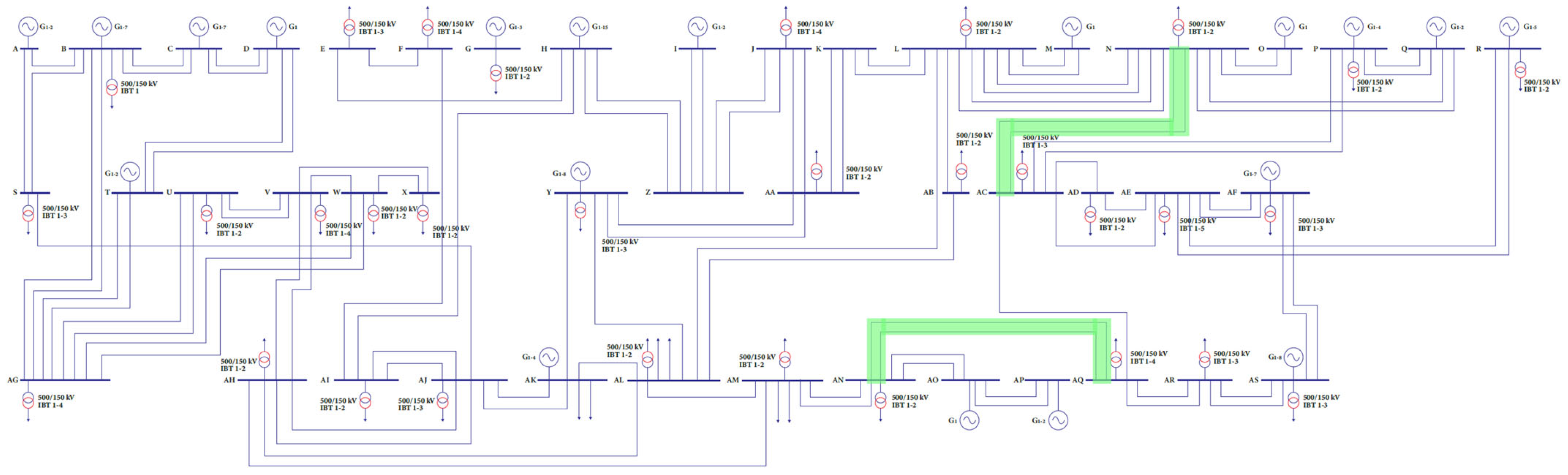
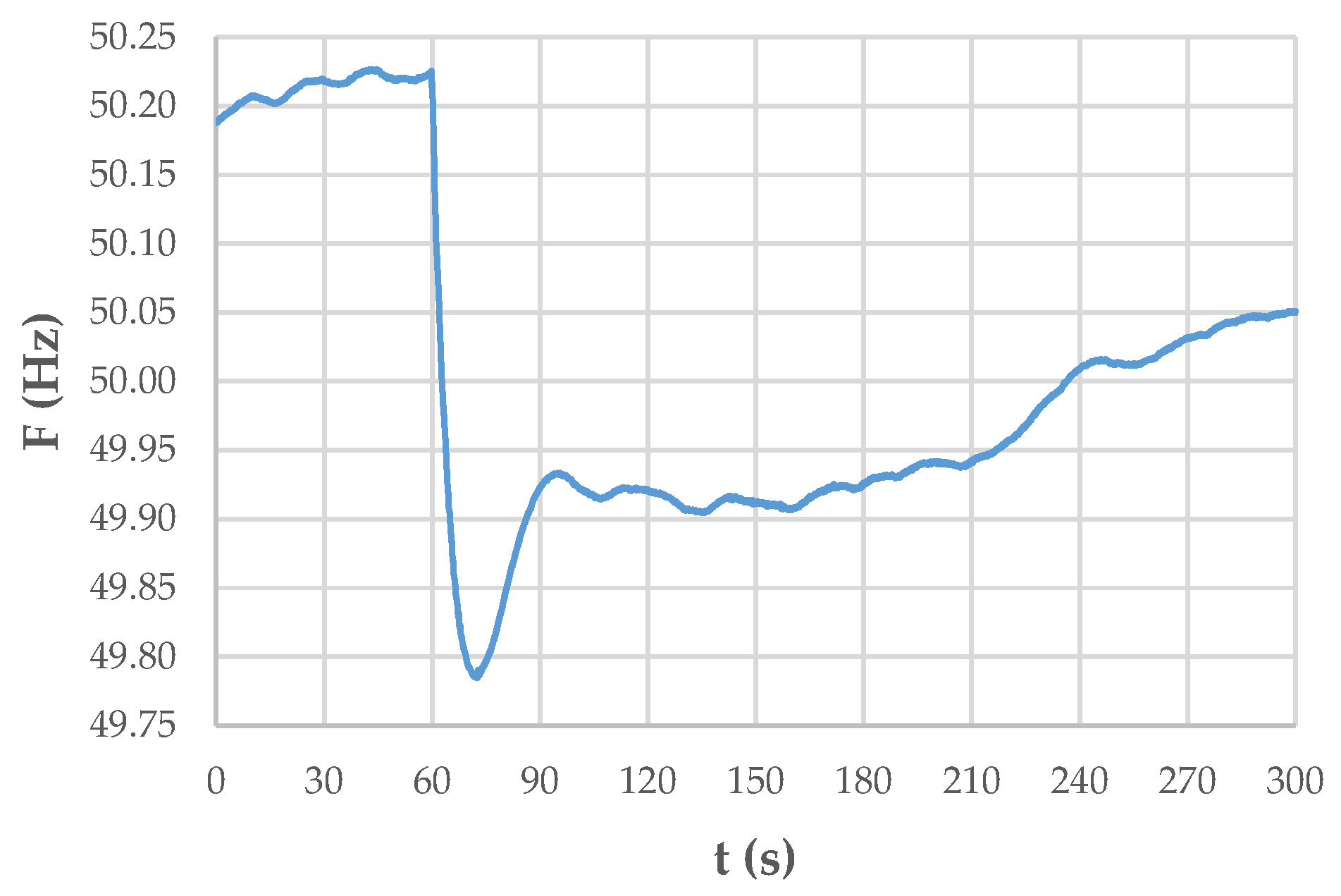
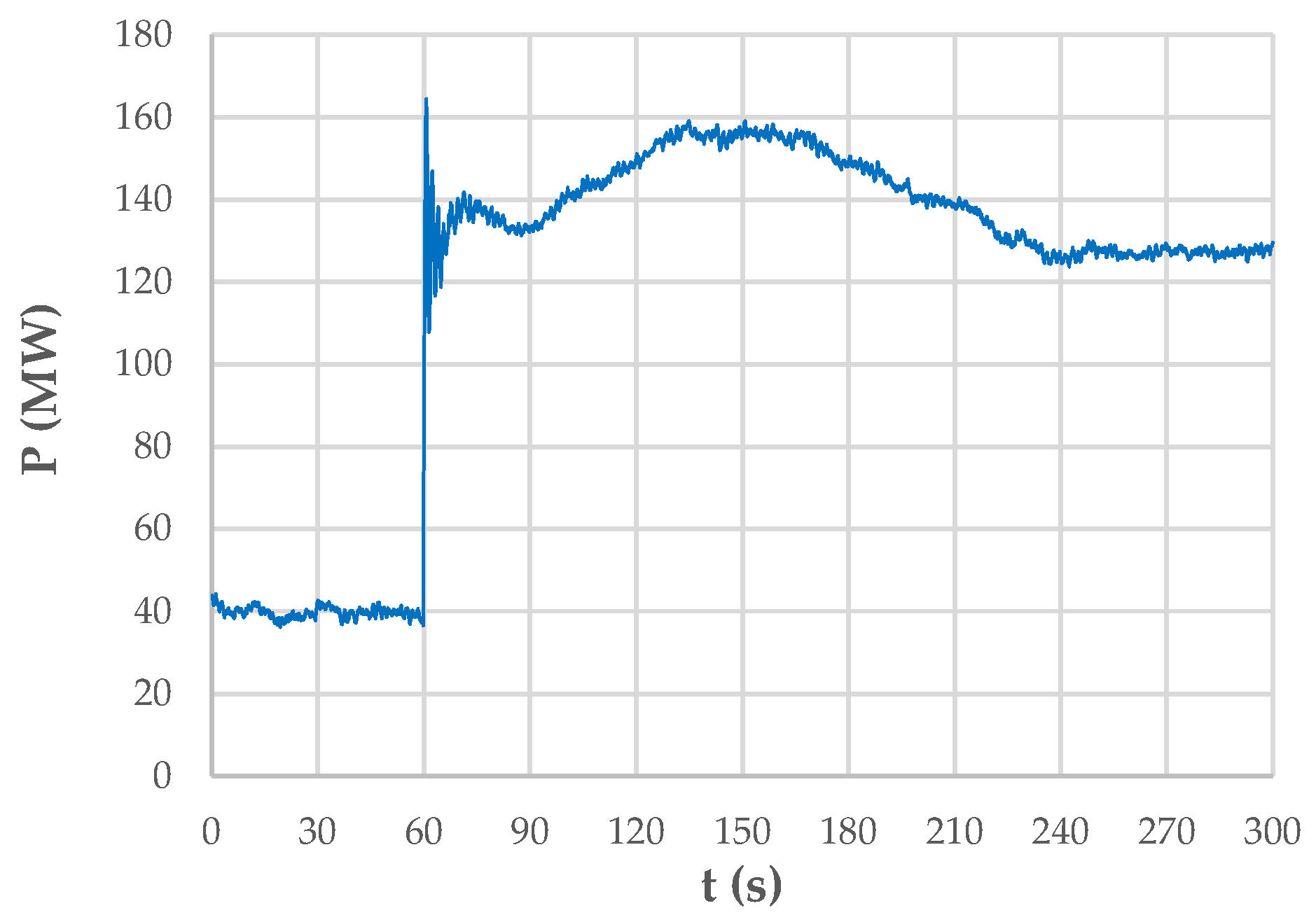
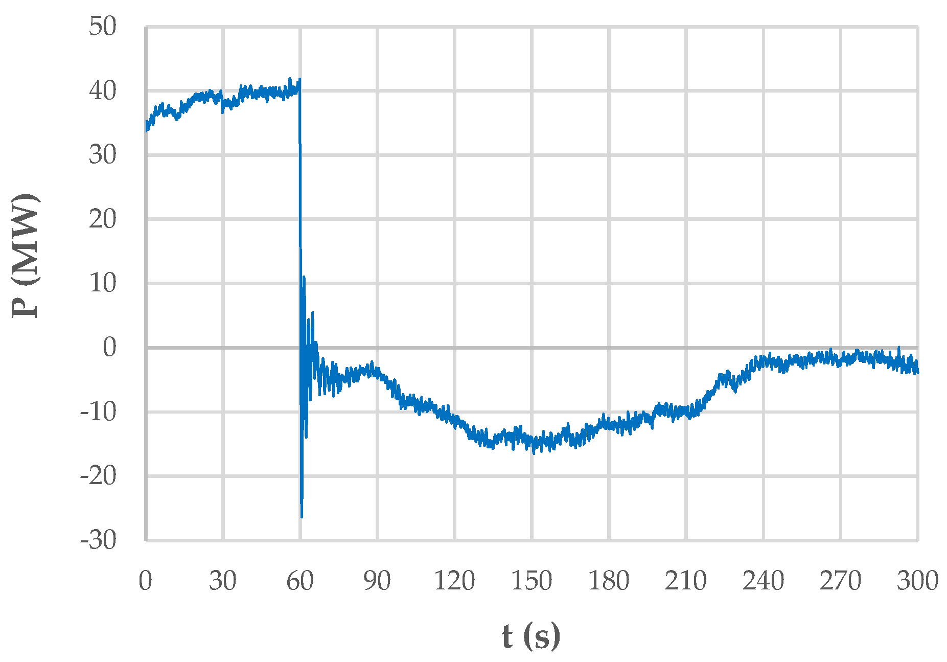
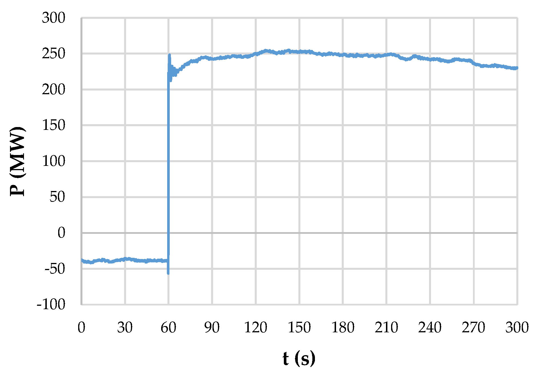
3.1. Case Study

The real PMU measurements were performed in a real 500 kV Java Bali grid system, as illustrated in Figure 6. This system includes 45 extra-high-voltage (EHV) substations that act as simplified buses, connecting a total generation capacity of 40,000 MW and a peak load of 32,000 MW across 6794 km of circuit lines. The 500 kV grid is further segmented into smaller subsystems that provide power to the 150 kV grid system through interbus transformers. PMUs were installed at each bus within the interconnected 500 kV power system.
There is an event taken as a case study for PMU measurements: the load rejection test. A load rejection test is a well-planned test, a procedure conducted in a power plant to assess the performance and stability of generators when there is a sudden reduction in electrical load. This test aims to evaluate the ability of the generator and the control systems to handle load changes, ensure system stability, prevent damage, and validate the operational capacity of the power plant during abrupt load reductions.
During this test in the 500 kV grid system, a load rejection was carried out at one of the generators in bus I, which generated 880 MW out of the total load of 30,000 MW (approx. 3% of the load). The power system’s frequency dropped from 50.227 Hz to 49.875 Hz in less than 15 s before ramping up to 49.93 within 25 s, then oscillating, as shown in Figure 7. The measurement also detected the damped oscillation during this event.
In these tests, the PMU measurement was set at rate of 25 frames per second. Observations were carried out on all 500 kV buses. There was quite a significant change in power transfer on the northern and southern corridor of the interconnection system.
In the northern corridor, which is represented by the AC-to-N bus line, the power flow was initially in the sending mode of 40 MW. After the load rejection event, there was an increase in deliveries reaching 120 MW and oscillations in the higher-frequency spectrum in less than 10 s, along with some low-frequency spectrum, and it took around 170 s to return to steady-state conditions, as shown in Figure 8.
Meanwhile, power transfer in the southern corridor via the AN-to-AQ bus line altered from sending mode to receiving, as shown in Figure 9. The receiving power varies and oscillates at low frequencies in the range of approx. 15 MW.
An additional case was taken from bus J to H, where the power is initially in receiving mode as shown in Figure 10. There is an abrupt and notable step change at t = 60 s, where power quickly rises from negative to over 250 MW. This points to a significant system event, and there was a load rejection test. The power stabilizes at about 250 MW following the abrupt change, with slight variations suggesting slight system oscillations or dynamic adaptations to the disruption. In power system stability research, this kind of response is common, since the system experiences small-signal and transient oscillations before stabilizing into a steady-state operation.
As well as the power profile acquired from bus AN to bus AQ, power oscillations from bus AC to bus N also contain higher-frequencies spectra which may result from the measurement errors that are negligible since the main interest in this research is the low-frequency oscillation.
Although the inclusion of additional variables such as environmental conditions, photovoltaic (PV) output fluctuations, and dynamic load variations could enhance the comprehensiveness of oscillation analysis, the present study focuses on a specific load rejection event within the 500 kV Java power system. During this event, the influence of variable renewable energy (VRE) sources and environmental factors was minimal due to the controlled testing conditions and the dominance of conventional generation sources. To reinforce this context, the installed generation mix in the Java region, based on official 2024 national electricity data, is presented as follows: 65.38% coal-fired power plants, 26.31% gas- and diesel-based plants, 4.68% geothermal, 0.52% hydropower, and less than 0.01% combined from solar, wind, and biomass. This confirms the system’s heavy reliance on thermal generation, thereby justifying the exclusion of PV-related and environmental variability in the oscillation analysis.

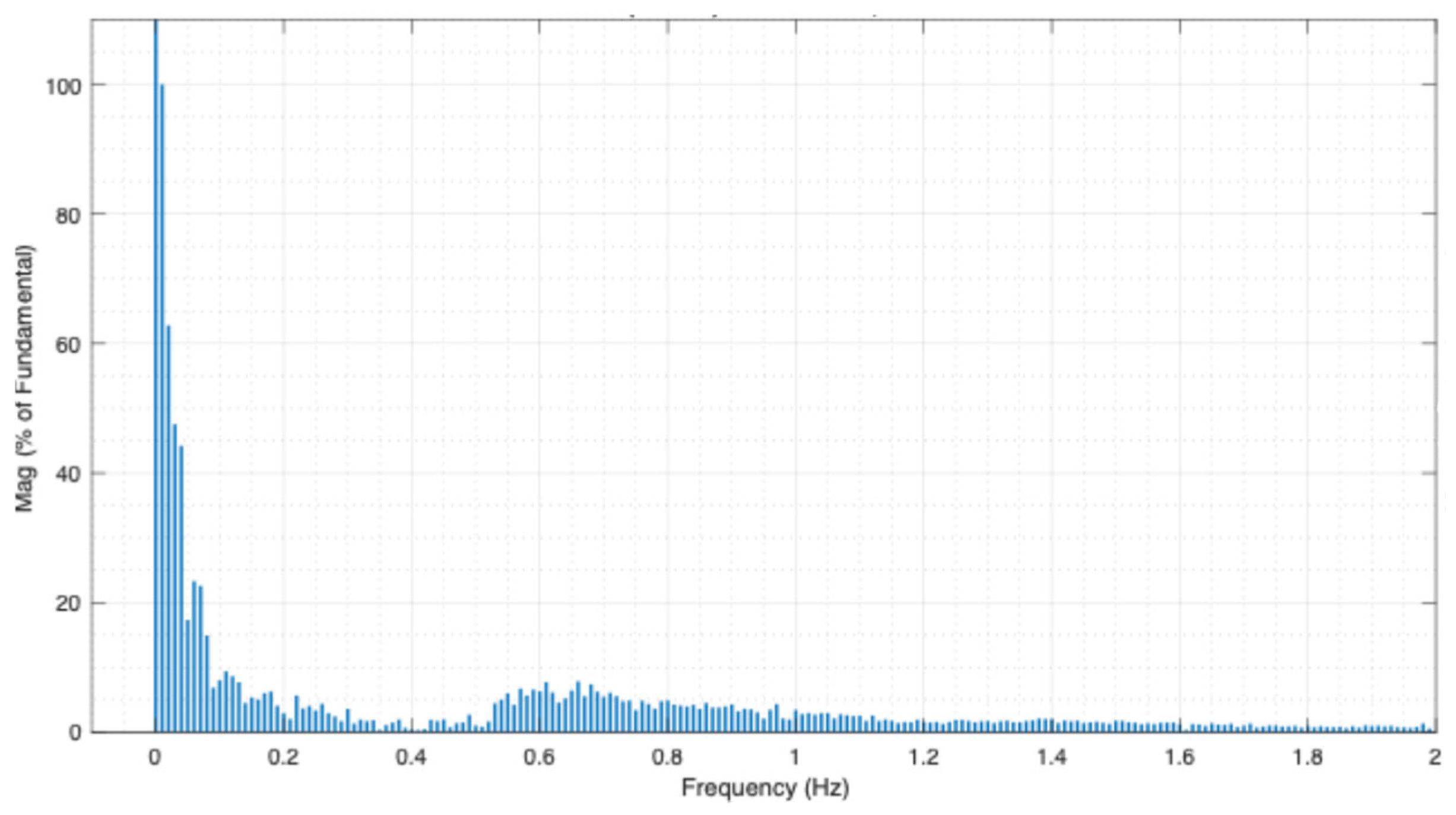
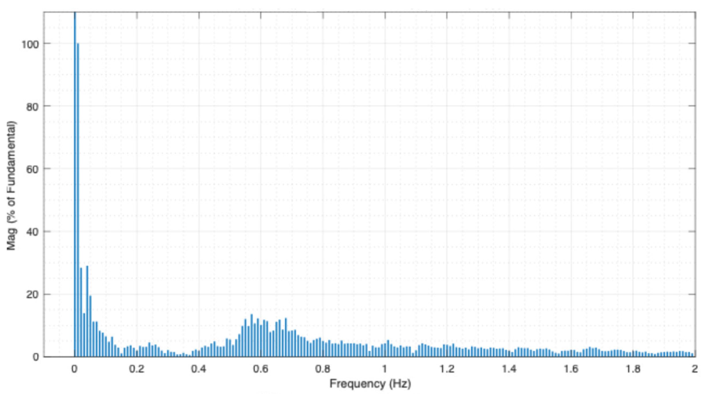
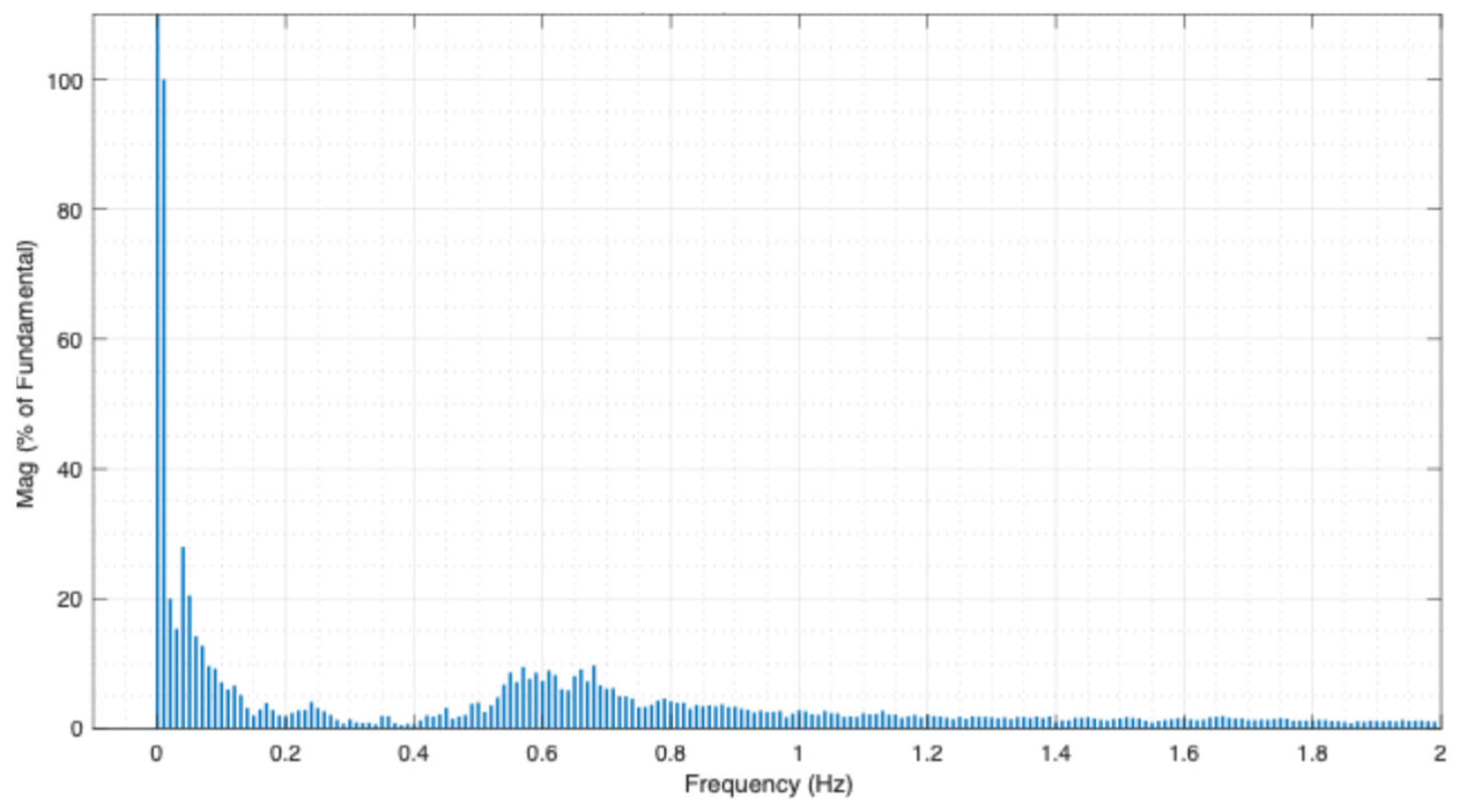
3.2. Low-Frequency Identification via FFT

FFT was employed to assess power transfer in bus AC to N, bus AN to AQ, and bus J to H during the load rejection test to analyze and identified the dominant spectrum. A time-domain signal with a chosen FFT window (highlighted in red) for spectrum analysis is shown in Figure 11, Figure 12 and Figure 13. The y-axis shows the signal’s magnitude, and the x-axis shows time in seconds. Around 50 s in, the signal experiences a sudden disturbance (load rejection test) that causes brief oscillations after initially maintaining a reasonably low and consistent magnitude. Following this, the signal gradually decreases towards the end of the timeline after stabilizing at a greater magnitude with slight fluctuations. The chosen time window for FFT analysis, which aids in identifying the oscillations’ frequency components, is represented by the red portion of the signal.
The three frequency domain plots depict the magnitude of oscillations at different frequencies in a power system. There are discernible oscillatory components between 0.2 and 0.8 Hz, which are suggestive of problems with small-signal stability, especially interarea oscillations in power systems. Comparing the three simulations as shown in Figure 14, Figure 15 and Figure 16, some differences can be detected in the magnitude of oscillations within the 0.2–0.8 Hz band. Stronger electromechanical interactions in the system are suggested by bus AC-N and bus AN-AQ, which seem to have somewhat larger oscillation magnitudes than bus J-H. This can be a sign of changes in the operating conditions of the system, control settings, or dampening effectiveness. Power system stabilizers (PSSs) or other control techniques may be necessary to improve system stability if higher oscillation magnitudes in this range indicate inadequate damping. These frequency components are essential for small-signal stability because they dictate how well the power system bounces back from minor disruptions. Prolonged power swings caused by poorly damped oscillations in the 0.2–0.8 Hz range might lower system reliability. Although the three graphs display comparable features, the oscillation magnitude variations point to distinct system responses, which could be brought about by adjustments to the control parameters, load circumstances, or generation. To ascertain the precise reason for these variations and to guarantee sufficient damping for stable operation, a more thorough examination of the system’s dynamics would be required.
The findings of an FFT simulation that examined power oscillations at various buses in a case study after a load rejection event are shown in Table 1. It gives the oscillatory modes’ frequency and amplitude at three different points: AC-N, AN-AQ, and J-H. The oscillation frequencies, which are common for local or interarea electromechanical modes in power systems, fall between 0.55 Hz and 0.68 Hz. Varying modes and buses have varying oscillation amplitudes, which are given as a percentage of the fundamental component.
When compared to the other buses, AN-AQ shows the strongest oscillations, with the largest oscillation amplitudes, reaching 13.4% at 0.57 Hz. Additionally, AC-N exhibits comparatively large oscillation amplitudes, especially at 0.68 Hz with 9.7%. With values between 7.4% and 7.8%, J-H exhibits the smallest amplitude oscillations. All buses exhibit consistent modes between 0.66 and 0.68 Hz, which points to a system-wide oscillatory mode that impacts various network segments.
Based on these findings, it can be said that following a load rejection event, the power system exhibits low-frequency oscillations between 0.55 and 0.68 Hz, with different buses exhibiting varied damping properties. Comparable oscillation frequencies among buses point to interrelated dynamic behaviors, highlighting the necessity of coordinated system-wide dampening solutions for stability.
While this study focuses on analyzing power system oscillations based on a load rejection event, it is important to acknowledge that such events represent only one type of system disturbance. To further validate the applicability and robustness of the Prony method, future research should consider a broader range of perturbation scenarios, including short-circuit faults, generator or unit switching, and line outages. These events often introduce more complex and abrupt dynamic responses that could challenge the stability and accuracy of oscillation detection methods. Expanding the study to include such scenarios, either through actual disturbance recordings or using digital real-time simulators and event playback techniques, would help verify the generalizability of the proposed approach and support its integration into more comprehensive grid monitoring frameworks.

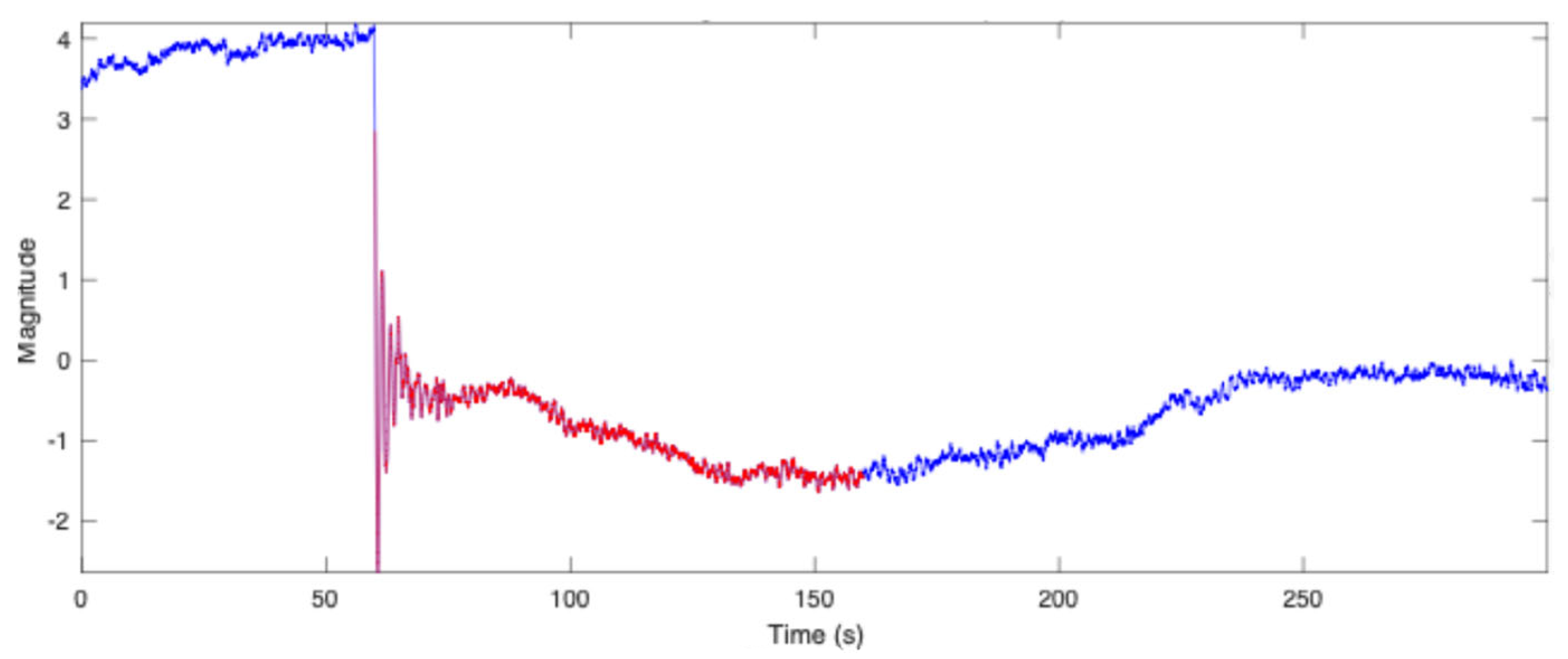
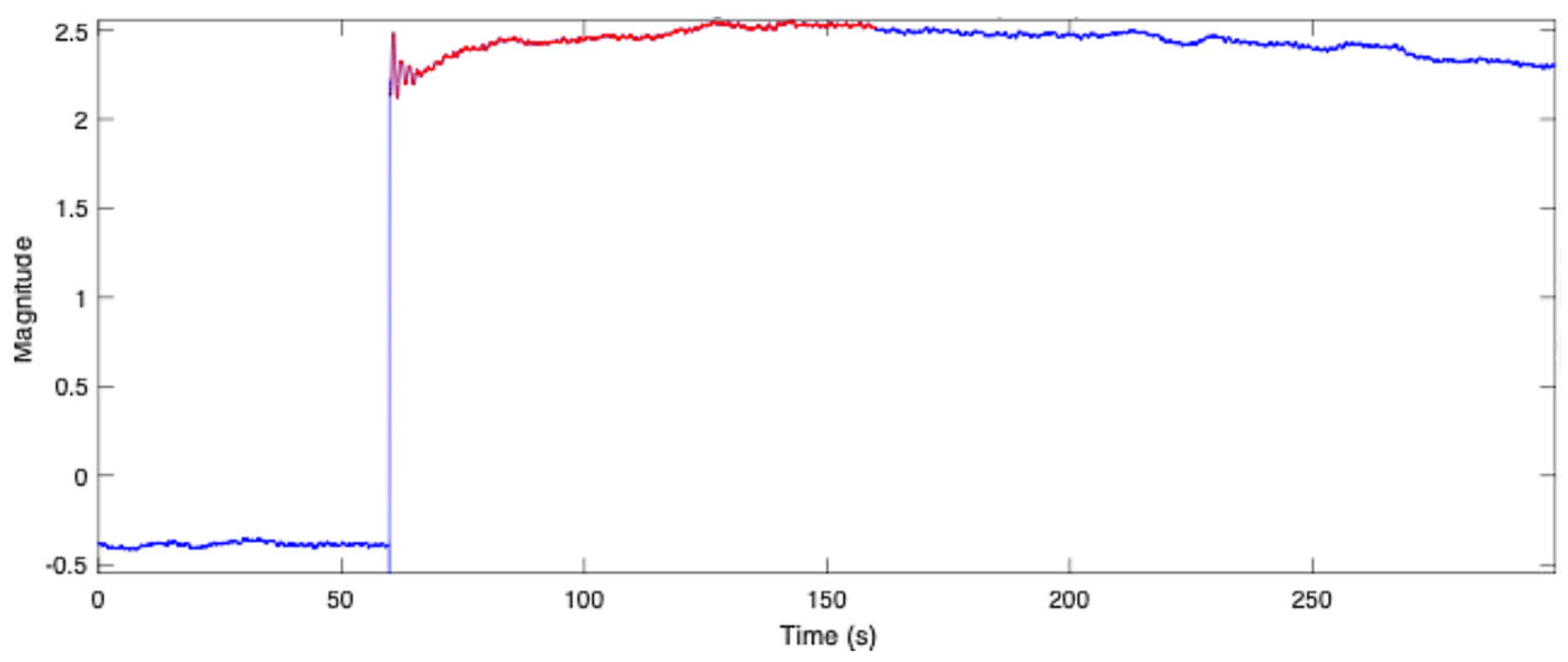
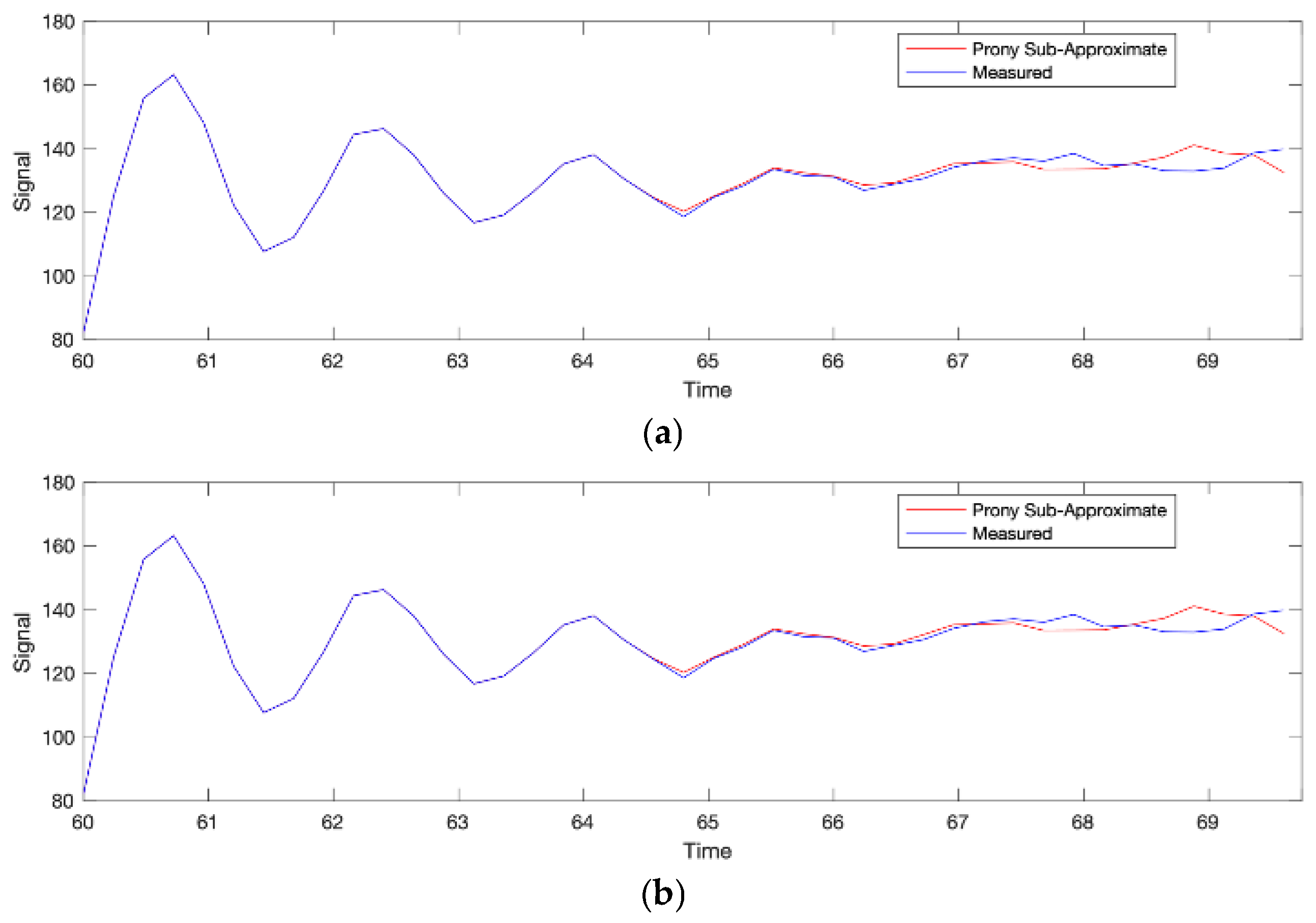
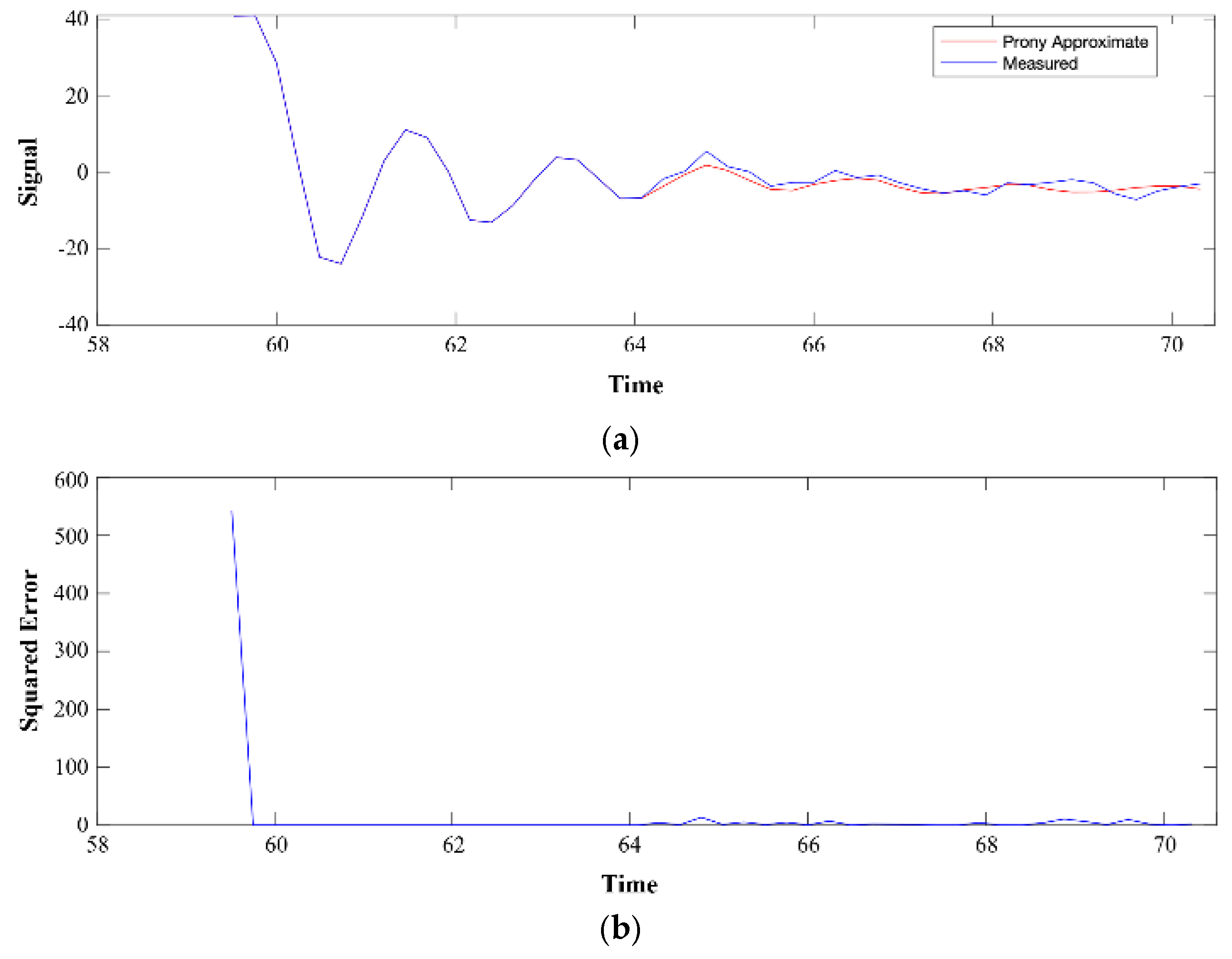
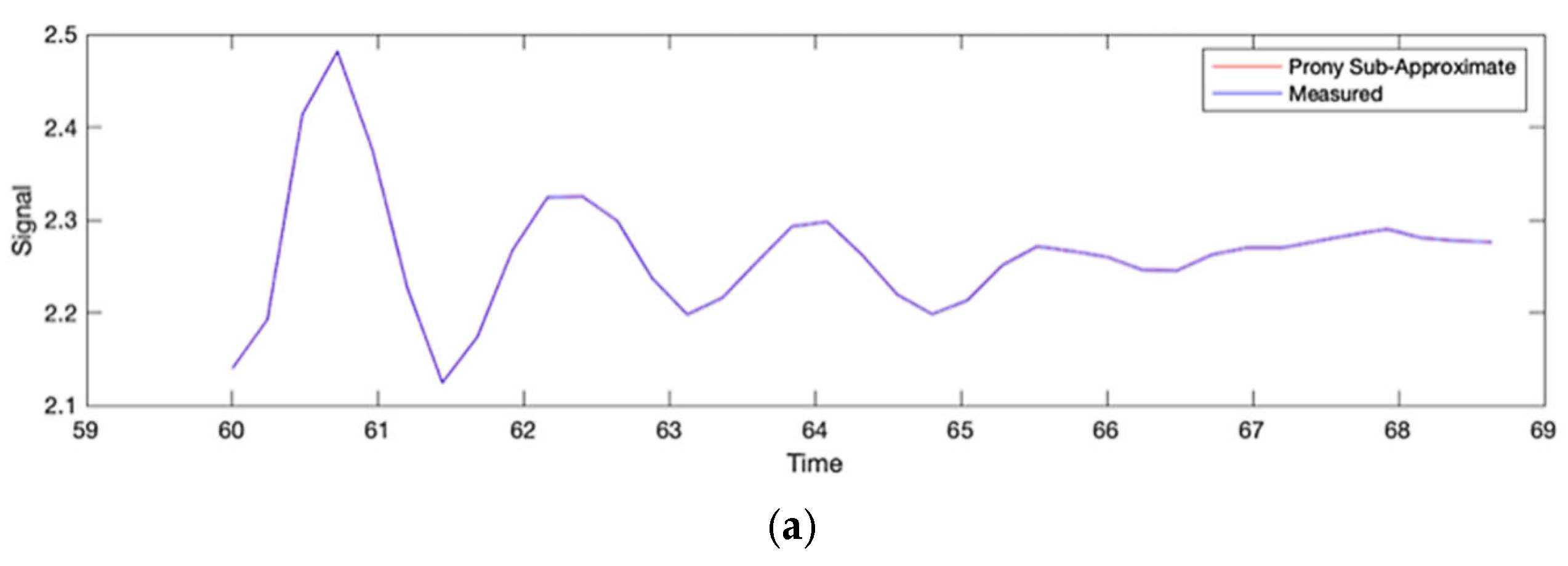
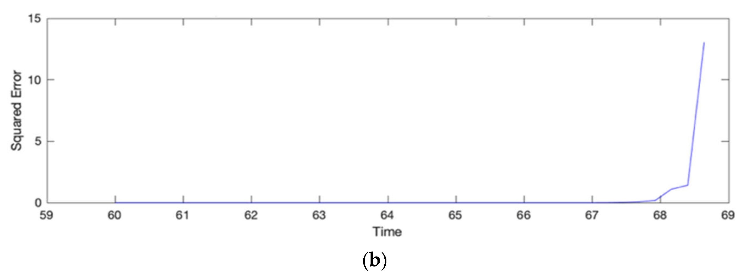
3.3. Low-Frequency Identification Using Prony’s Method

Power oscillations in a power system can be monitored during real-time analysis for parameters such as damping ratio and frequency to identify the mode shape of poorly damped electromechanical oscillations in wide areas using PMU measurements. Figure 17 shows Prony’s analysis of system responses following incidents or disturbances in the system during the load rejection test with power transfer, as shown in Figure 8.
For model order 18 and picking 18 with data range adjustments at t = event and DSF = 6, which process data from the power oscillation from Bus AC to Bus N, Prony’s analysis delivers a satisfying outcome, as shown in Figure 17a, where the measured data from the system (blue) and constructed by Prony’s approximation show good agreement. The squared error in Figure 17b started to rise after 67 s at the end of the power oscillation. The high squared error at the end of Prony’s approximation reaches >60% and still can be considered insignificant to the actual error at ~8%.
Table 2 shows Prony’s results of the load rejection test for the power oscillation from bus AC to bus N. Modes 1, 2, and 3, respectively, refer to the corresponding oscillation frequencies: 0.61 Hz, 1.7 Hz, and 0.77 Hz. Still, in the same case study, mode 1 corresponds to interarea oscillation, while mode 2 and mode 3 indicate the machine mode. The interarea oscillation for mode 1 has a large power oscillation, i.e., 510 MW, while the damping factor of 0.44 is sufficient, and for the machine modes in modes 2 and 3, the damping of 0.73 and 0.28 is sufficient to reduce the power oscillation to 4.8 MW and 3.7 MW.
For model order 18 and picking 17 with data range adjustments at t = event and DSF = 6, which process data from the selected study case power oscillation from bus AN to bus AQ, Prony’s analysis delivers a satisfying result, as shown in Figure 18a, where the measured data acquired from the system (blue) and constructed by Prony’s approximation show good agreement. The squared error in Figure 18b drops from approx. 550% down to nearly zero and remains low throughout the measuring time within the damped oscillation to reach stability. The high squared error in the initial Prony’s approximation, mainly due to the pre-recording data processing error, shall be neglected.
Table 3 shows Prony’s simulation results of the load rejection test taken from the actual power system. When the incident occurs in the system, the PMU sends the data to the PDC and the PDC and then carries out moving time window analysis of the PMU measurements towards real-time Prony’s analysis and concludes the dominant low-frequency oscillation and the damping ratio.
Modes 1, 2, and 3, respectively, refer to the corresponding oscillation frequencies: 0.35 Hz, 0.55 Hz, and 0.8 Hz. In this load rejection test study case, mode 1 and mode 2 correspond to interarea oscillations, while mode 3 indicates the machine mode. The interarea oscillation for mode 1 has a large power oscillation; that is, 490 MW with the damping factor of 0.47 is sufficient, and for mode 2, the damping factor of 0.22 can reduce the power oscillation at 4.9 MW. As for mode 3, the machine mode has been satisfactorily damp with a factor of 0.57 and a power oscillation of 3.8 MW.
For model order 18 and picking 18 with data range adjustments at t = event and DSF = 6, which process data from the selected study case power oscillation from Bus J to Bus H, Prony’s analysis delivers a satisfying outcome, as shown in Figure 19a, where the measured data acquitted from the system (blue) and constructed by Prony’s approximation show good agreement. The squared error in Figure 19b started to rise after 68 s at the end of the power oscillation. The high squared error at the end Prony’s approximation reaches >10%.
Table 4 shows Prony’s simulation results of the load rejection case for the power oscillation from Bus J to Bus H. Modes 1, 2 and 3, respectively, refer to the corresponding oscillation frequencies: 0.62 Hz, 0.81 Hz, and 1.2 Hz. Still, in the same study case, mode 1 and mode 2 correspond to interarea oscillations, while mode 3 indicates the machine mode.
The interarea oscillation for mode 1 has quite a large power oscillation; that is, 25 MW with the damping factor of 0.42 is sufficient, while for mode 2, the damping factor of 0.51 can reduce the power oscillation at 5.6 MW. The machine mode has been satisfactorily damp with a factor of 0.46 and a power oscillation of 1.7 MW.
Although the Prony method is recognized for its potential in real-time monitoring applications, this study does not include a detailed computational performance analysis to support that claim. At this stage, the real-time applicability discussed is based on the algorithmic structure and known advantages of Prony’s formulation in dynamic signal analysis. However, its practical feasibility can vary depending on the number of modes estimated, signal length, sampling rate, and the hardware environment used. Future work should therefore include a dedicated computational benchmarking study to evaluate its execution time, memory usage, and scalability.

4. Conclusions

When FFT and Prony’s analytic techniques are compared in the context of oscillations in the real power system interconnection, clear benefits and drawbacks of each method are revealed. As can be seen in the FFT analysis, major oscillatory modes at frequencies between 0.55 Hz and 0.68 Hz gives frequency domain representations of power oscillations. Although they do not directly reveal damping properties, the amplitude changes across buses show the strength of oscillations. However, Prony’s study offers more information in addition to frequency and amplitude, including damping factors. For example, bus AC-N shows that the dominant mode at 0.61 Hz has a damping factor of 0.44 and a considerable amplitude of 510 MW. Similar to this, bus AN-AQ shows weak damping for oscillations at 0.35 Hz and 0.55 Hz, suggesting a possible risk of prolonged oscillations. The higher frequency modes (e.g., 1.2 Hz) have comparatively smaller amplitudes but different damping levels, according to the bus J-H.
Comparatively speaking, FFT is good at detecting oscillatory modes but is inadequate for evaluating stability because it does not provide information on damping. However, Prony’s approach is more helpful for assessing system stability because it offers both frequency and damping information. Further stability control techniques are required, as indicated by the existence of weakly damped modes (e.g., damping < 0.3) in Prony’s results.
In conclusion, Prony’s approach offers a more thorough evaluation, especially for comprehending system stability and damping behavior, even though FFT is helpful for first spectral analysis. Combining the two techniques improves power systems’ capacity to identify and reduce low-frequency oscillations.

Author Contributions

Conceptualization, D.F.D., N.H. and B.A.S.; methodology, D.F.D. and I.K; software, I.K.; investigation, D.F.D., J.M. and I.K.; writing—original draft preparation, D.F.D. and I.K.; writing—review and editing, J.M. and K.M.B.-N.; supervision, K.M.B.-N., N.H. and B.A.S. All authors have read and agreed to the published version of the manuscript.

Funding

This research received no external funding.

Data Availability Statement

The raw data supporting the conclusions of this article will be made available by the authors on request.

Conflicts of Interest

Author Joko Muslim and Indra Kurniawan were employed by the company PT PLN (Persero). The remaining authors declare that the research was conducted in the absence of any commercial or financial relationships that could be construed as a potential conflict of interest.

Abbreviations

The following abbreviations are used in this manuscript:
BOBlackout
CTsCurrent Transformers
CVTsCapacitive Voltage Transformers
DFTDiscrete Fourier Transform
DRTSDigital Real-Time Simulators
DSFDown Sampling Factor
EMSEnergy Management System
FFTFast Fourier Transform
GPSGlobal Positioning System
IEEEInstitute of Electrical and Electronics Engineers
NERCNorth American Electric Reliability Corporation
PDCPhasor Data Concentrator
PMUPhasor Measurement Unit
PSSsPower System Stabilizers
PTsPotential Transformers
PVPhotovoltaic
ROCOFRate of change of frequency
SCADASupervisory Control and Data Acquisition
UTCCoordinated Universal Time
VREVariable Renewable Energy
VTsVoltage Transformers

References

  1. Lai, L.L.; Zhang, H.T.; Mishra, S.; Ramasubramanian, D.; Lai, C.S.; Xu, F.Y. Lessons learned from July 2012 Indian blackout. In Proceedings of the 9th IET International Conference on Advances in Power System Control, Operation and Management (APSCOM 2012), Hong Kong, 18–21 November 2012; pp. 1–6. [Google Scholar] [CrossRef]
  2. Gou, B.; Zheng, H.; Wu, W.; Yu, X. Probability Distribution of Power System Blackouts. In Proceedings of the 2007 IEEE Power Engineering Society General Meeting, Tampa, FL, USA, 24–28 June 2007; pp. 1–8. [Google Scholar] [CrossRef]
  3. Yamashita, K.; Li, J.; Zhang, P.; Liu, C.-C. Analysis and control of major blackout events. In Proceedings of the 2009 IEEE/PES Power Systems Conference and Exposition, Seattle, WA, USA, 15–18 March 2009; pp. 1–4. [Google Scholar] [CrossRef]
  4. Hiyama, T.; Suzuki, N.; Funakoshi, T. On-line identification of power system oscillation modes by using real time FFT. In Proceedings of the 2000 IEEE Power Engineering Society Winter Meeting. Conference Proceedings (Cat. No.00CH37077), Singapore, 23–27 January 2000. [Google Scholar] [CrossRef]
  5. Guo, S.; Zhao, Y.; Song, J.; Zhang, S.; Liu, H. Analysis of Forced Power Oscillation Based on FFT. IOP Conf. Ser. Earth Environ. Sci. 2019, 223, 012020. [Google Scholar] [CrossRef]
  6. Li, H.; Li, Z.; Halang, W.A.; Zhang, B.; Chen, G. Analyzing Chaotic Spectra of DC–DC Converters Using the Prony Method. IEEE Trans. Circuits Syst. II Express Briefs 2007, 54, 61–65. [Google Scholar] [CrossRef]
  7. Feilat, E.A. Prony analysis technique for estimation of the mean curve of lightning impulses. IEEE Trans. Power Deliv. 2006, 21, 2088–2090. [Google Scholar] [CrossRef]
  8. Yutthago, P.; Pattanadech, N. Improved Least-Square Prony Analysis Technique for Parameter Evaluation of Lightning Impulse Voltage and Current. IEEE Trans. Power Deliv. 2016, 31, 271–277. [Google Scholar] [CrossRef]
  9. Zhao, S.; Loparo, K.A. Forward and Backward Extended Prony (FBEP) Method for Power System Small-Signal Stability Analysis. IEEE Trans. Power Syst. 2017, 32, 3618–3626. [Google Scholar] [CrossRef]
  10. Zhao, J.; Zhang, G. A Robust Prony Method Against Synchrophasor Measurement Noise and Outliers. IEEE Trans. Power Syst. 2017, 32, 2484–2486. [Google Scholar] [CrossRef]
  11. de la O Serna, J.A. Synchrophasor Estimation Using Prony’s Method. IEEE Trans. Instrum. Meas. 2013, 62, 2119–2128. [Google Scholar] [CrossRef]
  12. de la O Serna, J.A.; Martínez, E.V. Smart grids Part 2: Synchrophasor measurement challenges. IEEE Instrum. Meas. Mag. 2015, 18, 13–16. [Google Scholar] [CrossRef]
  13. Tawfik, M.M.; Morcos, M.M. On the use of Prony method to locate faults in loop systems by utilizing modal parameters of fault current. IEEE Trans. Power Deliv. 2005, 20, 532–534. [Google Scholar] [CrossRef]
  14. Pushkareva, A.V.; Markuleva, M.V. The Research of Noise Stability of the Prony’s Method While Processing of Cardiological Time Series. In Proceedings of the 2019 International Multi-Conference on Engineering, Computer and Information Sciences (SIBIRCON), Novosibirsk, Russia, 21–27 October 2019. [Google Scholar] [CrossRef]
  15. Zhao, M.; Yin, H.; Xue, Y.; Zhang, X.-P.; Lan, Y. Coordinated Damping Control Design for Power System with Multiple Virtual Synchronous Generators Based on Prony Method. IEEE Open Access J. Power Energy 2021, 8, 316–328. [Google Scholar] [CrossRef]
  16. Netto, M.; Mili, L. Robust Data Filtering for Estimating Electromechanical Modes of Oscillation via the Multichannel Prony Method. IEEE Trans. Power Syst. 2017, 33, 4134–4143. [Google Scholar] [CrossRef]
  17. Meyer, J.-U.; Burkhard, P.M.; Secomb, T.W.; Intaglietta, M. The Prony spectral line estimation (PSLE) method for the analysis of vascular oscillations. IEEE Trans. Biomed. Eng. 1989, 36, 968–971. [Google Scholar] [CrossRef]
  18. Sava, H.P.; McDonnell, J.T.E. Spectral composition of heart sounds before and after mechanical heart valve implantation using a modified forward-backward Prony’s method. IEEE Trans. Biomed. Eng. 1996, 43, 734–742. [Google Scholar] [CrossRef] [PubMed]
  19. Jafarpisheh, B.; Madani, S.M.; Jafarpisheh, S. Improved DFT-Based Phasor Estimation Algorithm Using Down-Sampling. IEEE Trans. Power Deliv. 2018, 33, 3242–3245. [Google Scholar] [CrossRef]
  20. Dai, R.; Liu, G.; Stability, S.-S. Graph Database and Graph Computing for Power System Analysis; IEEE: New York, NY, USA, 2024; pp. 365–389. [Google Scholar] [CrossRef]
  21. Vaccaro, A. Small-Signal Stability Analysis of Uncertain Power Systems. In Interval Methods for Uncertain Power System Analysis; IEEE: New York, NY, USA, 2023; pp. 87–94. [Google Scholar] [CrossRef]
  22. Sauer, P.W.; Pai, M.A.; Chow, J.H.; Stability, S.-S. Power System Dynamics and Stability: With Synchrophasor Measurement and Power System Toolbox; IEEE: New York, NY, USA, 2017; pp. 183–231. [Google Scholar] [CrossRef]
  23. Fan, L. Interarea Oscillations Revisited. IEEE Trans. Power Syst. 2017, 32, 1585–1586. [Google Scholar] [CrossRef]
  24. Vournas, C.D.; Metsiou, A.; Nomikos, B.M. Analysis of intra-area and interarea oscillations in South-Eastern UCTE interconnection. In Proceedings of the 2009 IEEE Power & Energy Society General Meeting, Calgary, AB, Canada, 26–30 July 2009; pp. 1–7. [Google Scholar] [CrossRef]
  25. Galassi, P.H.; de Almeida, A.B.; Pesente, J.R.; Ramos, R.A. Analysis of Wide-Area Input Signals for Damping Interarea Oscillation of the Interconnected Paraguayan-Argentinean System. In Proceedings of the 2021 14th IEEE International Conference on Industry Applications (INDUSCON), São Paulo, Brazil, 15–18 August 2021; pp. 1252–1257. [Google Scholar] [CrossRef]
  26. Jain, V.; Nagarajan, S.T.; Garg, R. Study of Forced Oscillations in Two Area Power System. In Proceedings of the 2018 2nd IEEE International Conference on Power Electronics, Intelligent Control and Energy Systems (ICPEICES), Delhi, India, 22–24 October 2018; pp. 96–101. [Google Scholar] [CrossRef]
  27. Mantzaris, J.C.; Metsiou, A.; Vournas, C.D. Analysis of Interarea Oscillations Including Governor Effects and Stabilizer Design in South-Eastern Europe. IEEE Trans. Power Syst. 2013, 28, 4948–4956. [Google Scholar] [CrossRef]
  28. Nomikos, B.M.; Kotlida, M.A.; Vournas, C.D. Interarea Oscillations and Tie-line Transients in the Hellenic Interconnected System. In Proceedings of the 2007 IEEE Lausanne Power Tech, Lausanne, Switzerland, 1–5 July 2007; pp. 68–73. [Google Scholar] [CrossRef]
  29. Mao, X.-M.; Zhang, Y.; Guan, L.; Wu, X.-C. Coordinated control of interarea oscillation in the China Southern power grid. IEEE Trans. Power Syst. 2006, 21, 845–852. [Google Scholar] [CrossRef]
  30. Breulmann, H.; Grebe, E.; Lösing, M.; Winter, W.; Witzmann, R.; Dupuis, P.; Houry, M.P.; Margotin, T.; Zerenyi, J.; Dudzik, J.; et al. Analysis and Damping of Inter-Area Oscillations in the UCTE/CENTREL Power System; Paper No 38-113; CIGRÉ: Paris, France, 2000. [Google Scholar]
  31. Available online: https://www.nerc.com/comm/RSTC_Reliability_Guidelines/Oscillation_Analysis_for_Monitoring_And_Mitigation_TRD.pdf (accessed on 20 March 2025).
  32. Available online: https://jdih.esdm.go.id/storage/document/PM%20ESDM%20No%2020%20Tahun%202020.pdf (accessed on 20 March 2025).
  33. Xu, Y.; Gu, Z.; Sun, K. Location and Mechanism Analysis of Oscillation Source in Power Plant. IEEE Access 2020, 8, 97452–97461. [Google Scholar] [CrossRef]
  34. Grigsby, L.L. (Ed.) Power System Stability and Control, 3rd ed.; CRC Press: Boca Raton, FL, USA, 2012. [Google Scholar] [CrossRef]
  35. Sharma, N.; Acharya, A.; Jacob, I.; Yamujala, S.; Gupta, V.; Bhakar, R. Major Blackouts of the Decade: Underlying Causes, Recommendations and Arising Challenges. In Proceedings of the 2021 9th IEEE International Conference on Power Systems (ICPS), Kharagpur, India, 16–18 December 2021; pp. 1–6. [Google Scholar] [CrossRef]
  36. Dinh, V.T.; Le, H.H. Vietnamese 500kV power system and recent blackouts. In Proceedings of the 2008 IEEE Power and Energy Society General Meeting—Conversion and Delivery of Electrical Energy in the 21st Century, Pittsburgh, PA, USA, 20–24 July 2008; pp. 1–5. [Google Scholar] [CrossRef]
  37. Pourbeik, P.; Kundur, P.S.; Taylor, C.W. The anatomy of a power grid blackout—Root causes and dynamics of recent major blackouts. IEEE Power Energy Mag. 2006, 4, 22–29. [Google Scholar] [CrossRef]
  38. Andersson, G. Causes of the 2003 major grid blackouts in North America and Europe, and recommended means to improve system dynamic performance. IEEE Trans. Power Syst. 2005, 20, 1922–1928. [Google Scholar] [CrossRef]
  39. Agustriadi; Sinisuka, N.I.; Banjar-Nahor, K.M.; Bésanger, Y. Modeling, Simulation, and Prevention of July 23, 2018, Indonesia’s Southeast Sumatra Power System Blackout. In Proceedings of the 2019 North American Power Symposium (NAPS), Wichita, KS, USA, 13–15 October 2019; pp. 1–6. [Google Scholar] [CrossRef]
  40. Meng, D.Z. China’s protection technique in preventing power system blackout to world. In Proceedings of the 2011 International Conference on Advanced Power System Automation and Protection, Beijing, China, 16–20 October 2011; pp. 1838–1844. [Google Scholar] [CrossRef]
  41. Singh, A.; Parida, S.K. Synchronized Measurement of Power System Frequency and Phase Angle Using FFT and Goertzel Algorithm for low-cost PMU Design. In Proceedings of the 2019 IEEE PES Innovative Smart Grid Technologies Europe (ISGT-Europe), Bucharest, Romania, 29 September–2 October 2019; pp. 1–5. [Google Scholar] [CrossRef]
  42. Zhang, S.; Tian, B.; Liang, J.; Cheng, Y. Detection of Harmonic Components using the FFT and Instantaneous Reactive Power Theory. J. Phys. Conf. Ser. 2022, 2242, 012034. [Google Scholar] [CrossRef]
  43. Witzmann, R.; Rittiger, J.; Winter, W. Inter-Area Oscillations during Development of Large Interconnected Power Systems. In Proceedings of the CIGRE Symposium, Working Plant and Systems Harder, London, UK, 7–9 June 1999. [Google Scholar]
  44. Kundur, P. Power System Stability and Control; McGraw-Hill: New York, NY, USA, 1994. [Google Scholar]
  45. IEEE C37.118.1-2011; IEEE Standard for Synchrophasor Measurements for Power Systems (Revision of IEEE Standard C37.118-2005). IEEE Standards Association: Piscataway, NJ, USA, December 2011.
  46. Gou, B.; Zheng, H.; Wu, W.; Yu, X. The Statistical Law of Power System Blackouts. In Proceedings of the 2006 38th North American Power Symposium, Carbondale, IL, USA, 17–19 September 2006; pp. 495–501. [Google Scholar] [CrossRef]
  47. Scutariu, M.; MacDonald, M. Industrial power system protection against transmission system blackouts. In Proceedings of the 2009 44th International Universities Power Engineering Conference (UPEC), Glasgow, UK; 2009; pp. 1–5. [Google Scholar]
  48. Ilic, M.D.; Allen, H.; Chapman, W.; King, C.A.; Lang, J.H.; Litvinov, E. Preventing Future Blackouts by Means of Enhanced Electric Power Systems Control: From Complexity to Order. Proc. IEEE 2005, 93, 1920–1941. [Google Scholar] [CrossRef]
  49. Chakraborty, N.C.; Banerji, A.; Biswas, S.K. Survey on major blackouts analysis and prevention methodologies. In Proceedings of the Michael Faraday IET International Summit 2015, Kolkata, India, 12–13 September 2015; pp. 297–302. [Google Scholar] [CrossRef]
  50. Phadke, A.G.; Thorp, J.S.; Adamiak, M.G. A new measurement technique for tracking voltage phasors, local system frequency, and rate of change of frequency. IEEE Trans. Power Appl. Syst. 1983, 102, 1025–1038. [Google Scholar] [CrossRef]
  51. Phadke, A.G.; Thorp, J.S. Synchronized Phasor Measurements and Their Applications, Softcover Reprint of Hardcover, 1st ed.; Springer: Berlin/Heidelberg, Germany, 2008. [Google Scholar]
  52. de la O Serna, J.A.; Martin, K. Improving phasor measurements under power system oscillations. IEEE Trans. Power Syst. 2003, 18, 160–166. [Google Scholar] [CrossRef]
  53. Macii, D.; Petri, D.; Zorat, A. Accuracy analysis and enhancement of DFT-based synchrophasor estimators in off-nominal conditions. IEEE Trans. Instrum. Meas. 2012, 61, 2653–2664. [Google Scholar] [CrossRef]
  54. Barchi, G.; Macii, D.; Petri, D. Accuracy of one-cycle DFT-based synchrophasor estimators in steady-state and dynamic conditions. In Proceedings of the 2012 IEEE International Instrumentation and Measurement Technology Conference (I2MTC), Graz, Austria, 13–16 May 2012; pp. 1529–1534. [Google Scholar]
  55. Gholami, A.; Chari, M.V.K. Enhanced Prony analysis using regularization techniques for oscillation mode estimation. IEEE Trans. Power Syst. 2020, 35, 1346–1354. [Google Scholar]
  56. Wang, Y.; Zhao, L.; Zhang, H. Robust damped sinusoids estimation using a modified matrix pencil approach. Electr. Power Syst. Res. 2021, 194, 107027. [Google Scholar]
  57. Liu, J.; Liu, Y.; Wang, Z. A hybrid Prony and neural network approach for oscillation analysis in wide-area monitoring systems. IEEE Access 2022, 10, 12345–12356. [Google Scholar]
  58. Zhang, X.; Sun, K.; Xu, Y. Deep learning-based dynamic mode decomposition for power system oscillation monitoring. Appl. Energy 2023, 335, 120732. [Google Scholar]
Figure 1. Power system protection and operating time.
Energies 18 02377 g001
Figure 3. Phasor monitoring configuration.
Energies 18 02377 g003
Figure 4. Original signal from the simulation/measurement.
Energies 18 02377 g004
Figure 5. Signal decomposition using Prony’s analysis.
Energies 18 02377 g005
Figure 6. Jawa–Bali 500 kV grid system configuration.
Energies 18 02377 g006
Figure 7. Frequency response of the 880 MW load rejection test (PMU Data).
Energies 18 02377 g007
Figure 8. Power transfer at one of the circuit response from bus AC to bus N when load rejection tests were carried out (PMU Data).
Energies 18 02377 g008
Figure 9. Power transfer response from bus AN to bus AQ when load rejection tests were carried out (PMU Data).
Energies 18 02377 g009
Figure 10. Power transfer response from bus J to H when load rejection tests were carried out (PMU Data).
Energies 18 02377 g010
Figure 11. Selected signal from bus AC to N for FFT analysis.
Energies 18 02377 g011
Figure 12. Selected signal from bus AN to AQ for FFT analysis.
Energies 18 02377 g012
Figure 13. Selected signal from bus J to H for FFT analysis.
Energies 18 02377 g013
Figure 14. FFT result from power oscillation bus AC-N.
Energies 18 02377 g014
Figure 15. FFT result from the power oscillation from bus AN-AQ.
Energies 18 02377 g015
Figure 16. FFT results from the power oscillation from bus J-H.
Energies 18 02377 g016
Figure 17. Load rejection test power oscillation from bus AC to bus N and Prony’s analysis results of model order 18 and picking 18 residues with data range adjustments at t = event and DSF = 6 with (a) Prony’s approximation of signals in the time domain; (b) squared error.
Energies 18 02377 g017
Figure 18. Load rejection test power oscillation from bus AN to bus AQ and Prony’s analysis results of model order 18 and picking 17 residues with data range adjustments at t = event and DSF = 6 with (a) Prony’s approximation of signals in the time domain; (b) squared error.
Energies 18 02377 g018
Figure 19. Load rejection test power oscillation from bus J to bus H and Prony’s analysis results of model order 18 and picking 18 residues with data range adjustments at t = event and DSF = 6 with Prony’s approximation of signals in the time domain (a); squared error (b).
Energies 18 02377 g019aEnergies 18 02377 g019b
Table 1. FFT result of load rejection test: power oscillation.
BusModeFrequency [Hz]Amplitude
[% Fundamental]
AC-N1 (interarea)0.579.5
2 (interarea)0.669.1
3 (interarea)0.689.7
AN-AQ1 (interarea)0.5511.9
2 (interarea)0.5713.4
3 (interarea)0.678.7
J-H1 (interarea)0.617.7
2 (interarea)0.667.8
3 (interarea)0.687.4
Table 2. Prony’s result of the load rejection test: the power oscillation between bus AC and bus N when t = event and DSF = 6.
ModeFrequency [Hz]Amplitude [MW]Damping
1 (interarea)0.615100.44
2 (machine)1.74.80.73
3 (machine)0.773.70.28
Table 3. Prony’s result of the load rejection test: the power oscillation between bus AN and bus AQ when t = event and DSF = 6.
ModeFrequency [Hz]Amplitude [MW]Damping
1 (interarea)0.354900.47
2 (interarea)0.554.90.22
3 (machine)0.83.80.57
Table 4. Prony’s result of the load rejection test: the power oscillation between bus J and bus H when t = event and DSF = 6.
ModeFrequency [Hz]Amplitude [MW]Damping
1 (interarea)0.62250.42
2 (interarea)0.815.60.51
3 (machine)1.21.70.46
Disclaimer/Publisher’s Note: The statements, opinions and data contained in all publications are solely those of the individual author(s) and contributor(s) and not of MDPI and/or the editor(s). MDPI and/or the editor(s) disclaim responsibility for any injury to people or property resulting from any ideas, methods, instructions or products referred to in the content.

