Characteristics of Wind Profiles for Airborne Wind Energy Systems

Abstract

An airborne wind energy system (AWES) harvests wind at a higher altitude above conventional wind turbines using tethered flying devices. For the design and development of an AWES, we need to know the representative wind speed profile, and its temporal variation is also quite important for the optimization of operation control. This study investigates wind speed profiles up to 3000 m, utilizing ERA5 data spanning from 2000 to 2022 and measured data from a laser wind radar. The long-term averaged wind profile is statistically analyzed, as well as wind profiles with different cumulative probabilities, which are generally consistent with the logarithmic law. Statistical results show that the frequency of negative shear is more than 85% in instantaneous wind profiles, with a greater likelihood at altitudes between 500 m and 1500 m. Fluctuations in wind speed and direction based on 10 min averaged wind speed data have also been provided, which are described by a normal distribution. The wind speed fluctuations primarily concentrate within 2 m/s, with a standard deviation of approximately 0.45 m/s. The wind direction fluctuations are severe at the ground layer and show a rapid decay trend with increasing altitude and averaged wind speed. These results can support the design and control optimization of the AWES.

1. Introduction

Amid the challenges of global warming and the worsening energy crisis, researchers worldwide have devoted extensive efforts to developing new and efficient renewable energy sources, as alternatives to traditional fossil fuels. This endeavor has propelled remarkable progress in renewable energy technologies and industries, especially in the field of wind energy. In recent decades, airborne wind energy has emerged as a popular and potential field due to its advantages, such as larger energy reserves and higher power density [1,2,3,4,5], leading to the emergence of numerous cutting-edge technologies. Airborne wind energy systems (AWESs) primarily utilize tethered flying devices harvesting wind at higher altitudes beyond the reach of conventional wind turbines and converting wind energy into electricity [6,7]. In recent years, it has garnered significant attention from research institutions and enterprises globally [8,9,10,11], including notable projects like KiteGen in Italy [12,13], SkySails Power in Germany [14,15], the KitePower in the Netherlands [16], the Makani Power in the United States [17], and the parachute-based airborne wind energy system in China [18].

For the design and development of an AWES, we need to know the representative wind speed profile at the wind farm site. Although the preliminary design of an AWES may be based on a uniform and constant wind field [19] or an assumed wind profile [20,21,22,23], further optimization needs a better understanding of the high-altitude wind conditions. Some researchers focused on the assessment of high-altitude wind resources based on long-term observation and available wind reanalysis data. Archer and Caldeira [1] conducted an assessment of global wind energy resources between altitudes of 500 and 12,000 m based on NCEP reanalysis data. Subsequently, numerous scholars have performed detailed assessments of high-altitude wind resources in specific locations using more refined reanalysis datasets [5,24,25,26]. These studies provide valuable references for the site selection and planning of AWESs.

For a specific AWES project, the local wind profile and wind speed distribution play a critical role in operational strategies and control optimization, yet related research remains limited. Sommerfeld et al. [27] analyzed measured wind speed data below 1100 m in northern Germany and found significant differences in wind conditions under varying atmospheric stability, as well as different optimal operating heights and power outputs for simplified AWES models. Schelbergen et al. [28] proposed a wind profile clustering method to improve extrapolation accuracy. Sommerfeld et al. [29] clustered simulated 10 min wind speed profiles to derive representative wind profiles and analyzed their effects on AWES power, tether tension, and operational trajectories. Despite the ability of wind profiles and wind speed distributions to reveal long-term wind resource characteristics, they overlooked the short-term variations in wind.

Understanding the variation in wind conditions is quite important for the optimization of operation control to avoid tethers from becoming tangled together, especially for a wind farm with multiple AWES units. Given that existing AWES technologies often involve large-span, flexible tether structures or “kite” configurations operating at high altitudes, they are highly sensitive to fluctuations in wind speed and direction [10,30,31]. Abrupt changes in wind speed and direction may cause tethered flying devices to deviate from their intended trajectories or experience disorders, and, in the case of clusters, could lead to cable entanglement or even catastrophic failures [31,32]. Therefore, short-term wind characteristics must be given special attention to ensure the safety of AWES operations.

However, there are few studies about the negative shear frequency and temporal variations in high-altitude wind conditions. This necessitates high temporal-resolution wind data. Common methods for measuring high-altitude wind include radiosondes, tethered airships equipped with anemometers, and wind light detection and ranging (LiDAR) technology. Among these, LiDAR systems can offer continuous and uninterrupted observational capabilities and have been widely employed in wind resource assessments and evaluations at high altitudes [27,28,33,34,35,36]. A LiDAR system was installed at the AWES experimental site in Jixi County, Anhui Province, China, which provided basic data for this research.

With the aim of providing support for the design and development of AWESs, this research investigates the characteristics of high-altitude wind conditions up to 3000 m, especially on the statistically representative wind profiles and the fluctuations in wind speed and direction. The study is based on continuous observational data and ERA5 reanalysis datasets, and the data sources are briefly introduced in Section 2. The high-altitude wind profiles are then analyzed in Section 3, and the negative shear frequency is discussed. The fluctuations in wind speed and direction are statistically analyzed, and their variations with altitude are given in Section 4. Finally, conclusions are drawn in Section 5.

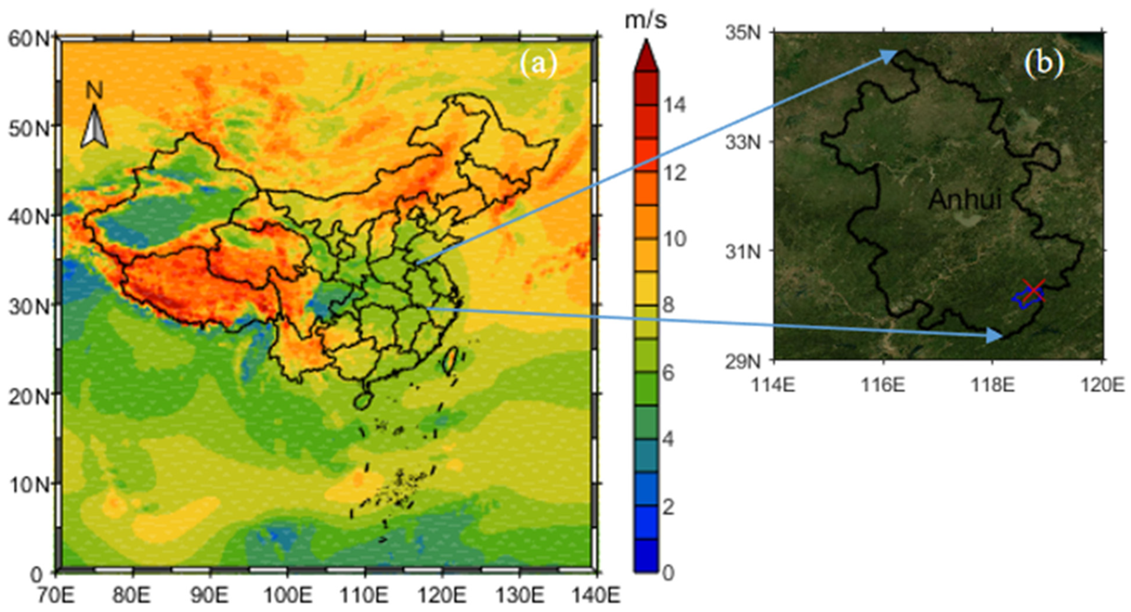
2. Data Sources and Methodology

A parachute-based airborne wind energy system has been established at an AWES experimental site, located in Jixi County, Anhui Province, China [18], which is chosen as the representative region to study the high-altitude wind conditions. The experimental site is located on open flat land in a suburban area with no nearby shelter. Figure 1 shows the location of the AWES experimental site and provides a general view of high-altitude wind resources at this site. The site is located in eastern China, where the long-term averaged high-altitude wind speed is approximately 7 m/s at 1500 m high [5]. The coordinates of the site are 118.75° E and 30.278° N, which is marked as a red X in Figure 1b.

We utilized the ERA5 reanalysis data provided by the European Centre for Medium-Range Weather Forecasts (ECMWFs) [37] to obtain the long-term statistical characteristics of the high-altitude wind profiles. ERA5 reanalysis data, with a temporal resolution of 1 h and a spatial resolution of 0.25°, have been validated by many researchers in combination with radiosonde data and meteorological station observations, demonstrating their suitability for analyzing averaged wind characteristics [38,39]. In this study, ERA5 data, spanning 23 years from 1 January 2000 to 31 December 2022, were employed, covering pressure levels from 600 hPa to 1000 hPa. Furthermore, two common wind profile curves were used to fit the mean profile, i.e., the power law model and the logarithmic law model. The power law model was proposed by Davenport [40] based on the compilation of a large number of near-surface wind profiles and can be expressed by the following equation:

$$U(Z)=U(Z_1){\left({\displaystyle \frac{Z}{Z_1}}\right)}^{\alpha }$$

(1)

where Z and U(Z) represent the height and the wind speed; Z₁ and U(Z₁) represent the reference height and its wind speed; and α is a power exponent representing the increase in wind speed with height.

According to the Monin–Obukhov similarity theory [41], the logarithmic law model can be expressed by the following equation under the neutral condition:

$$U(Z)={\displaystyle \frac{U_{\ast }}{\kappa }}\ln {\displaystyle \frac{Z}{Z_0}}$$

(2)

where κ represents the Kamen constant, generally taken as 0.4; and $U_{\ast }$ and Z₀ indicate the friction velocity and the roughness length.

LiDAR systems offer high temporal resolution for measuring the vertical distribution of wind in the atmosphere, effectively complementing the spatiotemporal density limitations of conventional high-altitude wind observations and reanalysis data. Data from a LiDAR system installed at the AWES experimental site have been utilized to analyze the fluctuation characteristics, which are obtained by first finding the 1 h smoothed wind speed and wind direction. Then, the fluctuations in wind speed and direction at each moment compared to the smoothed wind speed and direction are obtained according to Equations (3) and (4). Corrections for fluctuations in the vicinity of 0° and 360° of the instantaneous wind direction need to be taken into account in the treatment process.

$$\Delta u(t)=u(t)\cos \varphi +v(t)\sin \varphi -U$$

(3)

$$\Delta \varphi (t)=\varphi (t)-\varphi$$

(4)

where $\Delta u(t)$ and $\Delta \varphi (t)$ represent the fluctuations in wind speed and wind direction; u(t), v(t), and $\varphi (t)$ represent the 10 min wind speed component and wind direction; U represents the 1 h smoothed wind speed $U=\sqrt{{\overline{u}}^2+{\overline{v}}^2}$ and $\varphi$ represents the dominant wind direction $\varphi =\arccos {\displaystyle \frac{\mathrm{sign}(\overline{v})\overline{u}}{U}}$; and $\overline{u}$ and $\overline{v}$ represent the 1 h averaged wind speed component.

Two time periods with continuous measurements in April and November 2022 were adopted in this study. The measurement device employed Wind3D 6000, a Coherent Doppler Lidar (CDL) system, with a laser wavelength of 1.55 μm, a maximum detection range of 6 km, and a maximum wind speed measurement of 75 m/s. The wind speed measurement accuracy is 0.1 m/s, and the wind direction accuracy is no more than 3°. During the measurements, a radial distance resolution of 57 m was used, primarily focusing on 10 min averaged wind speeds between 100 m and 3000 m altitude.

Table 1. Key properties of two data sources.

Data Sources	Spatial Resolution	Temporal Resolution	Coverage	Intervals
ERA5	0.25°	1 h	1000~600 hPa	25/50 hPa
LiDAR	\	10 min	113~3020 m	57 m

summarizes the key properties of the ERA5 data and LiDAR data.

3. Wind Speed Profiles

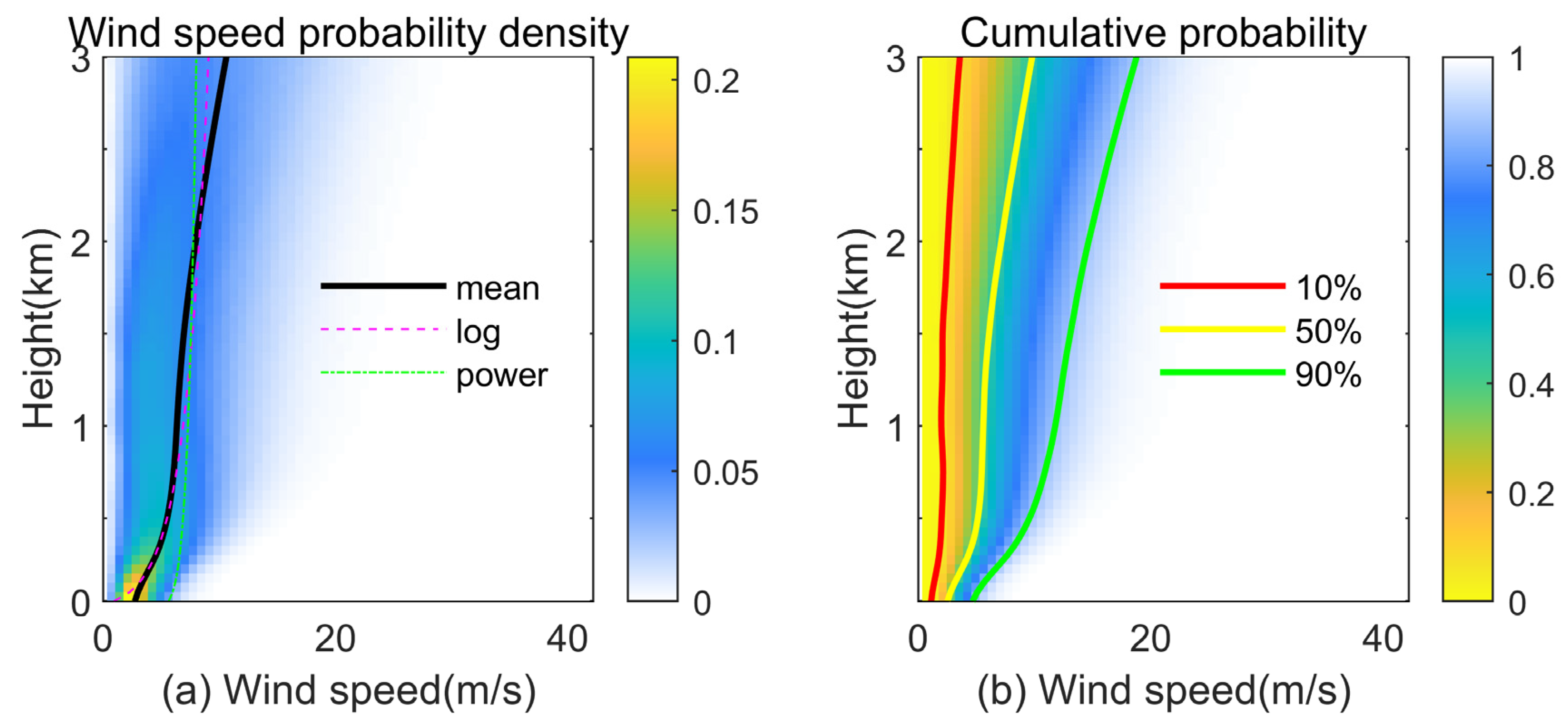
3.1. Long-Term Averaged Wind Profiles

Generally, the flying devices are designed to operate from the ground to 3000 m high in the parachute-based airborne wind energy system. Thus, the wind speed profile up to 3000 m is analyzed. Figure 2 presents the long-term averaged wind profile characteristics derived from ERA5 reanalysis data in Jixi County. This region exhibits substantial wind speed variations across vertical layers, with maximum surface wind speeds approximating 8 m/s and values exceeding 40 m/s at 3000 m. Figure 2a demonstrates the wind speed probability density. The background color shows the speed probability density at each altitude, and the black solid line shows the mean wind speed profile. Generally, the averaged wind speed shows an increasing trend with altitude. At the research site, it is approximately 3 m/s near the ground surface and 11 m/s at 3000 m. The predominant wind speeds remain below 10 m/s with infrequent occurrences of strong winds.

Comparative analysis of two fitted wind profile curves shows the superior overall performance of the logarithmic law over the power law. While extrapolation using logarithmic relationships with surface-layer winds enables reasonable estimation of upper-level winds, both models exhibit notable deviations above 2000 m. Thus, in the absence of reliable high-altitude wind data, the logarithmic law can be adopted as a preliminary approximation.

Figure 2b illustrates cumulative probability distributions, where red, yellow, and green curves respectively represent 10th, 50th (median), and 90th percentile wind speeds. These percentile distributions maintain consistent proportional relationships across various heights.

Table 2. Ratio to long-term averaged wind speed for different cumulative probability.

Height/m	5%	10%	25%	50%	75%	90%	95%
100	0.46	0.53	0.68	0.92	1.25	1.57	1.79
200	0.46	0.54	0.69	0.94	1.25	1.55	1.73
300	0.45	0.53	0.69	0.94	1.25	1.55	1.75
400	0.44	0.52	0.68	0.94	1.26	1.57	1.78
500	0.43	0.50	0.67	0.93	1.26	1.59	1.81
1000	0.35	0.43	0.61	0.89	1.29	1.73	2.00
1500	0.33	0.40	0.58	0.88	1.31	1.77	2.05
2000	0.31	0.40	0.58	0.91	1.32	1.75	2.00
2500	0.30	0.39	0.59	0.93	1.33	1.72	1.95
3000	0.30	0.39	0.60	0.94	1.34	1.69	1.91
Average	0.38	0.46	0.64	0.92	1.29	1.65	1.88

quantifies the ratios between percentile wind speeds and their averaged values at representative elevations. Key observations include the following: the 10th percentile winds range from 0.39 to 0.54 times the averaged values, displaying decreasing ratios with height (mean ratio ≈ 0.46); the 50th percentile winds are 0.88–0.94 times the averaged values, and the ratio is constantly oscillating in height (mean ratio ≈ 0.92); and the 90th percentile winds measure 1.55–1.77 times median values, exhibiting complex altitudinal variation: initial decrease followed by increase and subsequent reduction (mean ratio ≈ 1.65).

This characteristic ratio pattern persists across other percentiles. Although absolute values may vary regionally depending on mean wind conditions, the fundamental proportionality between percentile wind speeds at different altitudes remains consistent. Such relationships facilitate rapid assessment of local wind speed ranges and energy potential through vertical extrapolation of measured surface winds.

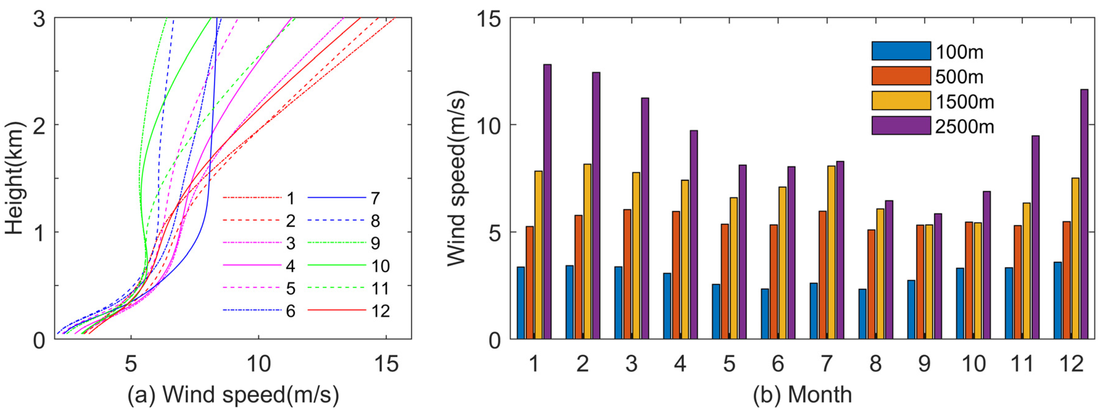
3.2. Monthly Variation in Wind Profiles

Wind conditions in the study area have significant seasonal variations, due to the influence of monsoons. Figure 3 presents the long-term averaged wind profile characteristics of Jixi County for each month, based on ERA5 data from 2000 to 2022. It is evident that the averaged wind profiles exhibit significant seasonal variations. Figure 3a shows the mean profile of each month over 23 years, where spring, summer, fall, and winter are represented by purple, blue, green, and red, respectively. Wind speeds are greatest overall in winter (greatest in July when near 1000 m) and maintain a trend of increasing with height and at the relatively greatest rate of increase. Wind profiles in spring are similar to those in winter but are smaller than in winter at high altitudes, and the difference increases with time. The wind profiles in summer are well characterized, showing a rapidly increasing trend with increasing height below 1000 m, but a slow increasing rate above 1000 m, and not much change at 3000 m, especially in July. In the fall, the wind profile shows an increasing trend both below 500 m and above 1500 m, but there is an obvious negative shear feature between 500 m and 1500 m. Overall, the wind energy potential is higher in spring and winter and slightly worse in summer and fall. The low growth trend of wind speed at high altitudes in summer and the negative shear feature in fall will seriously affect the operation and control strategy of an AWES, and it is possible that the power generation will be reduced instead when operating above 1500 m, so the maximum operating altitude needs to be carefully considered.

Figure 3b displays the monthly averaged wind speed bar charts at heights of 100 m, 500 m, 1500 m, and 2500 m. It is visually apparent that wind speeds generally increase with altitude across most months, with the largest variations occurring in winter and the smallest in September and October. Furthermore, the temporal distribution of near-surface wind speeds differs from that at higher altitudes. Near the surface, the lowest averaged wind speed at about 2.5 m/s occurs in June, while the highest at about 3.5 m/s is observed in December. In contrast, at 2500 m, the lowest averaged wind speed at about 5.8 m/s is recorded in September, and the highest at about 13 m/s in January. Moreover, the wind speed is maximum in July at 500 m and 1500 m, which may be due to the southeast monsoon.

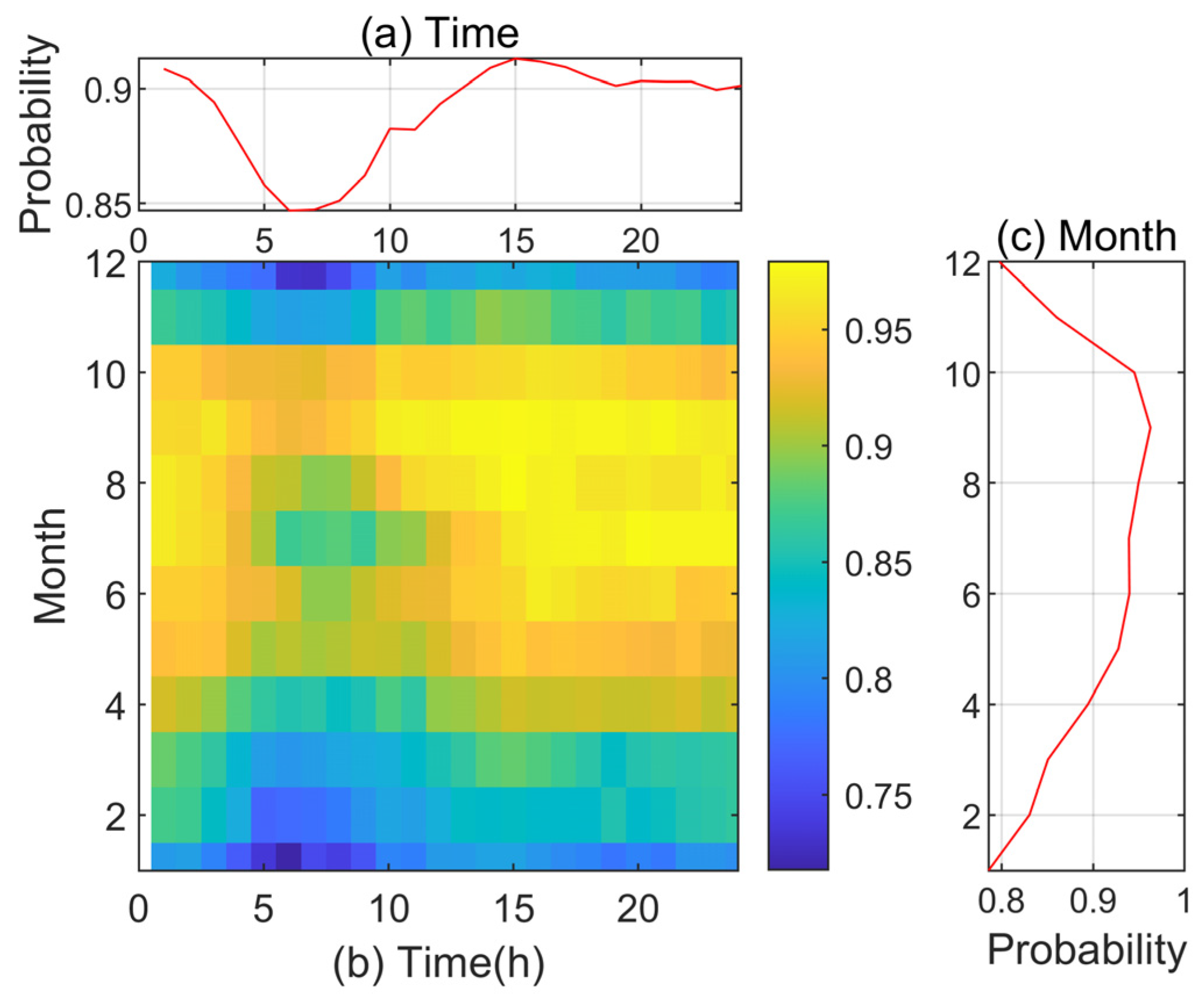
3.3. Occurrence Probability of Negative Wind Shear

Generally, the rising of flying devices generates power in the parachute-based airborne wind energy system, and a decrease in wind speed in the upper layer or the negative wind shear may lead to a sudden reduction in power generation and difficulty in system control. In Figure 3, the averaged wind profiles during autumn all show the phenomena of negative wind shear, indicating that many instantaneous wind profiles also exhibit the same phenomena. Figure 4 exemplifies randomly selected wind profiles exhibiting such negative shear phenomena, demonstrating their occurrence across a diverse altitude range from ground surface to 3000 m. It can be seen that wind speed can be quite low at high altitudes. Leveraging ERA5 multi-level reanalysis data, we systematically analyzed spatiotemporal patterns of negative shear through the following methodology: We counted wind speeds at 0.5 m/s intervals based on the raw data from ERA5. Whether or not negative wind shear occurs is determined in the following way: for each pressure layer and each moment, if the wind speed in the lower layer is greater than that in the upper layer, negative shear is considered to have occurred in this layer at this time. Statistical evaluation revealed that 85% of wind profiles exhibited negative shear signatures, though predominantly characterized by minor shear magnitudes.

With this treatment, the probability of negative wind shear for all pressure layers and wind speed intervals can be derived. Afterward, the probabilities are interpolated to different heights for a better presentation. Figure 5 delineates the probability characteristics of negative vertical wind shear across wind speed (Figure 5a) and altitude domains (Figure 5c). As illustrated in Figure 5b, the occurrence of negative vertical wind shear exhibits pronounced dependencies on both wind speed and altitude. The statistical probability of negative shear under all height layers shows a trend of increasing and then decreasing with wind speed in Figure 5a, about 0.075 in the 0–0.5 m/s wind speed interval, with the peak probability occurring near 4 m/s, about 0.32. The probability of negative shear begins to oscillate continuously with wind speeds exceeding 24 m/s, and the probability of exceeding 37 m/s is 0, which is due to the small probability of occurrence for large wind speeds, a small number of samples, and lack of statistical stability. Similarly, the sample of small wind speeds is relatively small, with the amount of data for 0–0.5 m/s being about 10% of the data at 4 m/s. Neglecting the case of very small wind speeds, it can be roughly assumed that the probability of negative wind shear inversely correlates with the magnitude of wind speeds.

As quantified in Figure 5c, the probability of negative wind shear shows a trend of rapid increase followed by slow decrease with increasing height. The probability does not exceed 0.1 below 200 m, and the peak probability of about 0.42 occurs near 1000 m. Above 2000 m, the probability varies less and basically stays near 0.24. The frequency reaches a maximum from 500 m to 1000 m at approximately 0.4 and remains less than 0.1 below 300 m. Wind speed has the greatest effect on the probability of negative shear, with a more concentrated probability gradient along the wind speed axis compared to the change in altitude. Taken together, the peak probability is concentrated within the range of wind speeds from 2 m/s to 6 m/s, which is the most susceptible wind speed range. And the most likely altitude range is 500 m to 1500 m.

In order to temporally characterize the distribution of negative wind shear, we counted it by month and time. For a given moment, negative shear is considered to occur at this moment in time, as long as negative shear occurs at any pressure level. Figure 6 statistically delineates the spatiotemporal occurrence patterns of negative vertical wind shear in Jixi County, with a marginal curve quantifying probability distributions across time (Figure 6a) and calendar months (Figure 6c). The occurrence probability of negative vertical wind shear exhibits significant seasonal modulation, with heightened prevalence observed during May, August, September, and October. Specifically, October demonstrates the maximum daily occurrence rate exceeding 95%, while winter months show a comparatively lower probability of approximately 80%. This temporal pattern aligns with the characteristics of monthly averaged wind profiles in Figure 3a, where long-term averaged wind profiles during August, September, and October exhibit explicit negative wind shear within 500 m to 1000 m. Temporal analysis reveals a diurnal modulation of negative shear occurrence probability. It can be divided into three phases as follows: (1) initial decline phase from 02:00 to 06:00 with gradual probability reduction; (2) recovery phase from 06:00 to 15:00; and (3) stabilization phase from 15:00 to 02:00. Among them, the lowest probability was reached near 06:00 of approximately 84%. The probabilities in the stabilization phase were all over 91%.

This distribution pattern is closely linked to atmospheric stability and diurnal mixing processes. During daytime, intense solar radiation enhances vertical mixing, leading to a more unstable atmosphere. Conversely, nocturnal conditions exhibit greater atmospheric stability [42]. Consequently, the probability of negative wind shear is relatively lower at night and higher during daylight hours. On longer timescales, reduced atmospheric stability in spring and winter corresponds to lower probabilities of such conditions, whereas the opposite trend prevails in the summer and autumn seasons.

While the analyses in this section are site specific, the proportional relationships between accumulated probability wind profiles exhibit fundamental consistency across mid-latitude regions [42,43], as do the distribution patterns of negative wind shear. However, their quantitative expressions demonstrate site-specific variations governed by local topographic and synoptic pattern influences.

4. Fluctuations in Wind Speed and Direction

In land-based AWESs, the periodic ascent and recovery of a flying device form a cyclic power generation mechanism [12,13,14,15,16,18]. Take the parachute-based airborne wind energy system as an example, a cycle of ascent and recovery typically lasts approximately 10 to 30 min. The variation in wind during the cycle has a significant impact on the stability of the system. In Section 3, we analyzed the long-term averaged wind profile characteristics of Jixi County based on ERA5 reanalysis data. However, reanalysis data are unable to capture short-term variations at the 10 min timescale. These features have significant implications for the control and operation of an AWES, such as cable reeling speed, the opening and closing of flying devices, maximum ascent height, flight direction, and trajectory. In extreme cases, such variations could potentially lead to cable entanglements or system failures in AWES clusters [31,32]. Therefore, measured data are used to obtain the fluctuation characteristics.

In this section, we analyze the short-term variation characteristics of wind speeds based on the observed high-altitude wind data from Jixi County. During the analysis, we decomposed the measured 10 min wind data into the 1 h smoothed wind using a vector decomposition method and statistically analyzed the short-term fluctuations in wind speed and wind direction characteristics.

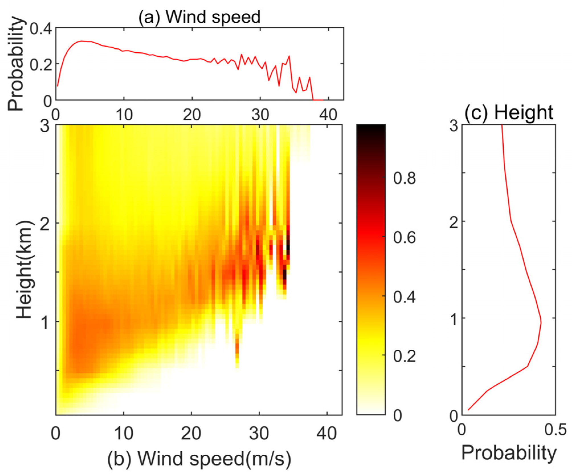
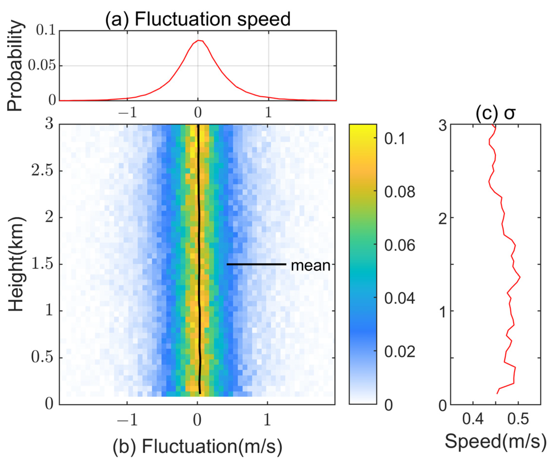
4.1. Characteristics of Fluctuations in Wind Speed

We obtain the longitudinal fluctuations in wind speed along the prevailing wind direction. Figure 7 illustrates the probability density of the measured wind speed at Jixi (Figure 7a) and the distribution of longitudinal fluctuations at 500 m (Figure 7b), 1500 m (Figure 7c), and 2500 m (Figure 7d). Figure 7a also illustrates the measured averaged wind profile (the black solid line) and the ERA5 averaged wind profile (the red solid line) for the same period. It can be observed that the two profiles generally agree well and exhibit slight differences below 1000 m, with the ERA5 wind profile showing a negative shear and being slightly higher than the measured results. Above 1000 m, both profiles demonstrate similar trends and patterns. In Figure 7b–d, the blue scatter points represent the fluctuation for each dataset, the red line represents the averaged fluctuation speed, the orange line represents the probability density of the smoothed wind speed, and the purple curve represents the probability density of the fluctuation speed.

As shown in the Figure 7, the hourly averaged wind speed ranges are 0–9 m/s, 0–11 m/s, and 0–13 m/s at the three altitudes, respectively. The longitudinal fluctuations at all three height levels are primarily concentrated within the range of −2 m/s to 2 m/s, with only a few outliers outside this range. The distribution of fluctuation speeds has good symmetry, but has high peaks near the averaged value of fluctuations (with a kurtosis exceeding 10). We tried to fit it with a normal distribution (not plotted in the figure), and the performance is slightly insufficient and does not well reflect the characteristic of the concentration of fluctuations. However, the fluctuations as a whole satisfy the two times standard deviation principle, which means that 95% of the data are within two standard deviations around the mean. In practical design, the fluctuation speed characteristics of 10 min relative to 1 h can be roughly distributed by the normal distribution. The standard deviations at each height are all approximately 0.46 m/s labeled in Figure 7, indicating that the standard deviation and distribution characteristics of fluctuations are consistent across different height levels.

Figure 8 presents the distributions of fluctuation in wind speed along height, with probability distributions across fluctuation (Figure 8a) and distribution of standard deviation along height (Figure 8c). To provide a more intuitive visualization of their vertical distribution, Figure 8b limits the x-axis to between −2 m/s and 2 m/s. The results indicate a higher probability density of absolute fluctuation speeds concentrated within 0.2 m/s, with a slightly lower probability between 0.2 m/s and 0.7 m/s, and fluctuations with an absolute value of more than 0.7 m/s are very sparsely distributed. Overall, the fluctuation speeds exhibit good symmetry and relatively concentrated distributions across all heights. Figure 8c provides the standard deviations of fluctuation speeds at different heights, which are consistently within the range of 0.42 m/s to 0.5 m/s. A gradual decreasing trend is observed as height increases, with the maximum standard deviation occurring near 1500 m. Similarly, transverse fluctuations can be computed in this way. But the distribution characteristics of transverse fluctuations are basically the same as those of longitudinal fluctuation speeds and are therefore not elaborated upon further.

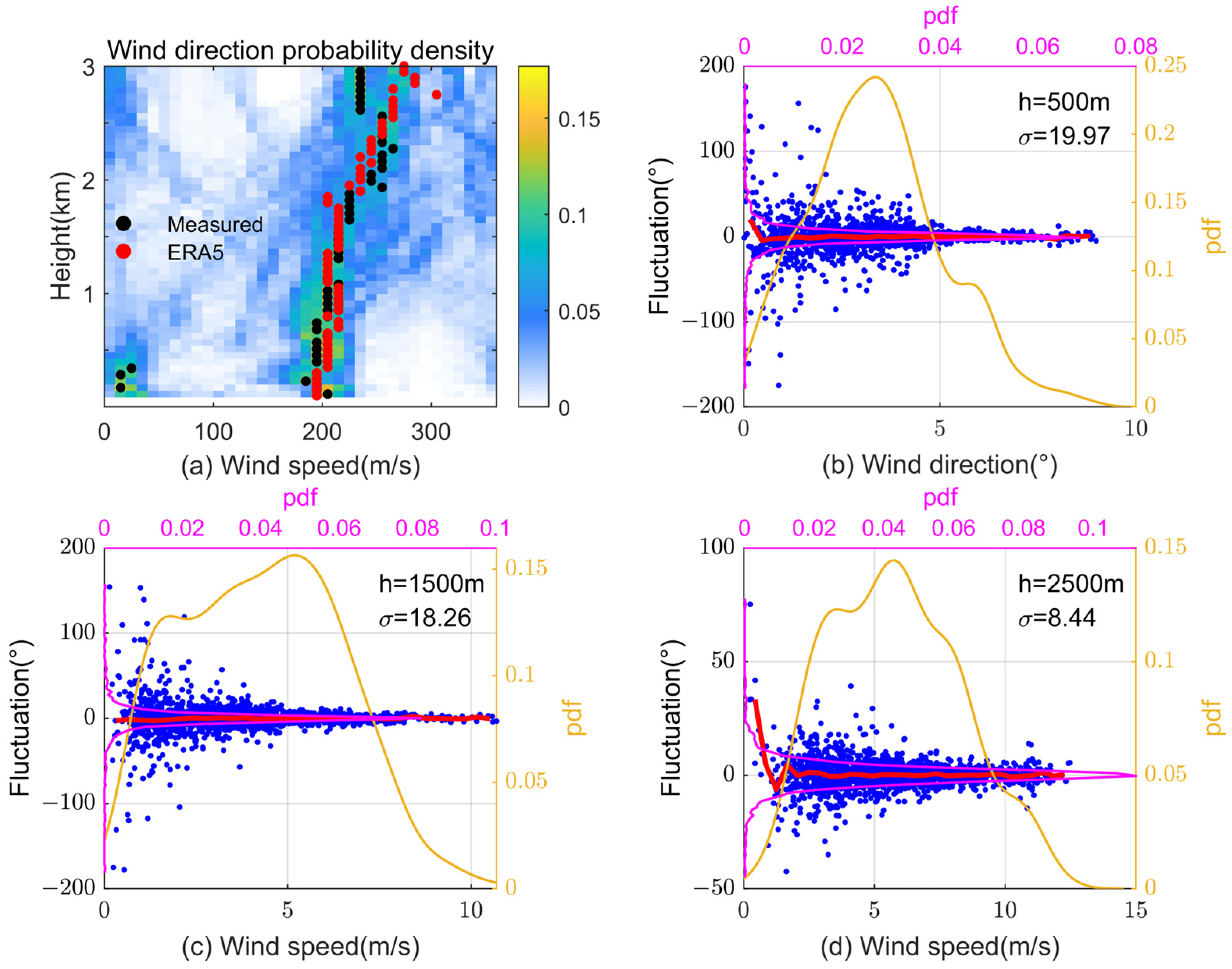
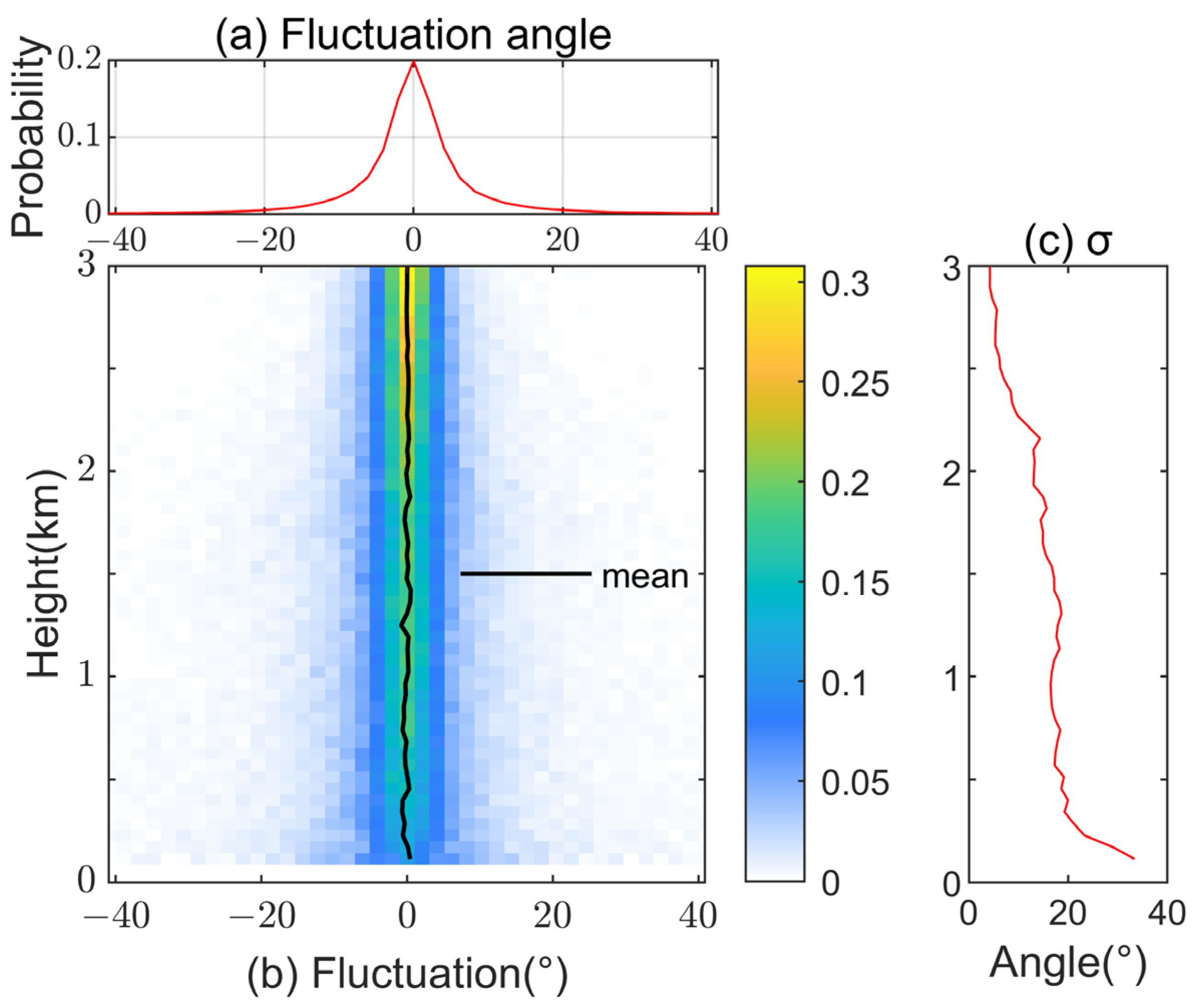
4.2. Characteristics of Fluctuations in Wind Direction

Similar to Section 4.1, Figure 9 illustrates the probability density of wind direction (Figure 9a) and the distribution of fluctuations in wind direction (Figure 7b–d). Figure 9a displays sector frequency analysis of the measured wind direction in 10° bins, where black dots denote the measured prevailing wind direction and red dots represent the contemporaneous ERA5 prevailing wind direction. The measured prevailing wind direction exhibits a progressive clockwise shift with increasing altitude, predominantly maintaining southwesterly orientations across most layers, except at a few heights. Below 500 m, wind directions cluster between 200° and 220° (southerly winds). From 500 m to 2000 m, the direction gradually shifts clockwise, transitioning to westerly winds (230–250°) above 2000 m. The ERA5-derived prevailing directions show strong agreement with measurements at lower altitudes but minor deviations at higher heights.

According to other subplots, it is observed that at low wind speed intervals (0–2 m/s), fluctuations exhibit a greater amplitude, with instances of approaching 180° wind direction reversal. Conversely, at higher wind speed intervals, fluctuations diminish and become more concentrated. Overall, the amplitude of fluctuations decreases with increasing height. In general, fluctuation characteristics are relatively consistent across different heights, with larger variability observed at lower wind speeds and smaller variability at higher wind speeds. This aligns with the findings in Section 4.1, where fluctuation speeds were primarily concentrated within the range of −2 m/s to 2 m/s. Additionally, as altitude increases, fluctuation angles diminish, indicating that wind direction at higher altitudes is more stable compared to near-surface levels. Similar to fluctuation speeds, fluctuation angles can be described using a normal distribution.

Figure 10 presents the vertical distributions of fluctuation angles along height, with probability distributions across fluctuation (Figure 10a) and distribution of standard deviation along height (Figure 10c). Higher probability densities occur within 10° of absolute fluctuation angles. Absolute fluctuation angles in the range of 10–20° have a low probability and are very sparse above 20°. Figure 10b quantifies the standard deviation of directional variation angles across altitudes, all remaining below 40°. These deviations decrease rapidly with height, exhibiting the steepest decline below 500 m (indicating highly variable near-surface winds). Between 500 m and 1500 m, the standard deviation stabilizes around 18°.

5. Conclusions

This study utilizes multi-year ERA5 reanalysis data and continuous high-altitude wind observation data to statistically analyze the wind profile up to 3000 m, supporting the design and optimization of AWESs. The long-term averaged wind speed profile can be well described by a logarithmic curve, and it was found that the wind speeds with different cumulative probabilities exhibit similar proportional relationships across different heights. Taking the averaged wind speed in Jixi County, the wind speed for 10% cumulative probability is approximately 0.46 times the averaged wind speed, while the 90% wind speed is approximately 1.65 times. This finding facilitates the rapid identification of primary wind speed ranges and the assessment of wind energy potential in the region. For some areas without long-term wind speed observation data, we can quickly estimate the wind speed range and simply evaluate the wind resource potential based on the proportional relationship between wind speed of different cumulative probability and averaged wind speed. For high-altitude wind speeds, high-altitude wind and its wind speed range can be quickly extrapolated based on near-ground observation data and logarithmic rate. And this can help AWES quickly determine suitable locations.

Additionally, the study revealed that negative wind shear is more prevalent during summer and autumn, particularly within wind speeds of 2–6 m/s and at altitudes between 500 m and 1500 m. In areas where negative shear occurs, the wind speed at the upper floor is smaller, which may reduce the power generation of some AWESs, or prevent the system from reaching the correct operating height, deviating from the set trajectory, etc. Therefore, when designing AWESs, relevant engineers need to consider the possible impact of negative shear and set control strategies or safety protection measures in advance, especially in summer and autumn and the range of 500 m to 1500 m.

Furthermore, the analysis of the 10 min wind speed data within a 1 h period indicated that longitudinal fluctuation speeds in the region are predominantly concentrated between −2 m/s and 2 m/s across all altitudes. The standard deviation of these fluctuations remains stable around 0.46 m/s. The fluctuation angle decreases with increasing altitude and averaged wind speed. The standard deviation diminishes from lower to higher altitudes, stabilizing within 18° above 500 m. The fluctuations in wind speed and wind direction can be described using a normal distribution, further supporting the statistical analysis of wind characteristics in the region. These results can provide a reference for the operating conditions that need to be considered in the design of AWESs. Relying solely on uniform wind fields or wind profiles may fail to identify potential issues with AWESs in variable wind conditions, such as cable tangling. We can construct diverse long-term wind conditions by superimposing fluctuating wind speeds and directions onto hourly average winds to validate the performance of AWESs, including power generation capabilities. By optimizing operational strategies, we can achieve maximum energy output under varying wind conditions.

It should be emphasized that the acquired long-term statistical characteristics are derived from ERA5 data in Jixi County, Anhui Province, China, while the fluctuation characteristics originate from field measurements conducted during April and November in this region. These characteristics can reasonably represent wind conditions in eastern China to a certain extent. It should be noted that the findings demonstrate geographical-specific limitations in temporal and spatial dimensions. Nevertheless, the identified patterns should maintain universal applicability across mid-latitude regions, although specific quantitative values may exhibit geographical variations.

The current research is very site specific. Future studies could explore other potential regions for high-altitude wind energy development, such as high-latitude areas, polar regions, and offshore locations. On the other hand, due to the relatively short time series of existing observational data, current analyses are confined to short-term fluctuation characteristics. Long-term statistical properties can only be investigated using reanalysis data, which may not be entirely accurate. Future work should utilize long-term continuous observational data to analyze genuine statistical characteristics. Furthermore, based on these findings, dynamic environmental wind fields could be constructed to conduct comprehensive simulation studies for various AWESs.

References

1. Archer, C.; Caldeira, K. Global assessment of high-altitude wind power. Energies 2009, 2, 307–319. [Google Scholar] [CrossRef]
2. IRENA. Future of Wind: Deployment, Investment, Technology, Grid Integration and Socio-Economic Aspects (A Global Energy Transformation Paper); International Renewable Energy Agency: Abu Dhabi, United Arab Emirates, 2019; Available online: https://www.irena.org/publications/2019/Oct/Future-of-wind (accessed on 11 December 2024).
3. Bechtle, P.; Schelbergen, M.; Schmehl, R.; Zillmann, U.; Watson, S. Airborne wind energy resource analysis. Renew. Energy 2019, 141, 1103–1116. [Google Scholar] [CrossRef]
4. EPO and IRENA. Patent Insight Report: Offshore Wind Energy; EPO: Vienna, Austria, 2023; Available online: https://www.irena.org/Publications/2023/Nov/IRENA-EPO-Offshore-Wind-Energy-Patent-Insight-Report (accessed on 11 December 2024).
5. He, H.; Niu, X.J. Spatial distribution of high-altitude wind energy resources in China. J. Hydroelectr. Eng. 2025, 44, 28–37. (In Chinese) [Google Scholar] [CrossRef]
6. Wijnja, J.; Schmehl, R.; De Breuker, R.; Jensen, K.; Vander Lind, D. Aeroelastic analysis of a large airborne wind turbine. J. Guid. Control. Dyn. 2018, 41, 2374–2385. [Google Scholar] [CrossRef]
7. Weber, J.; Marquis, M.; Cooperman, A.; Draxl, C.; Hammond, R.; Jonkman, J.; Lemke, A.; Lopez, A.; Mudafort, R.; Optis, M.; et al. Airborne Wind Energy; National Renewable Energy Laboratory: Golden, CO, USA, 2021. [CrossRef]
8. Thresher, R.; Robinson, M.; Veers, P. To capture the wind. IEEE Power Energy Mag. 2007, 5, 34–46. [Google Scholar] [CrossRef]
9. Williams, P.; Lansdorp, B.; Ockels, W. Optimal cross-wind towing and power generation with tethered kites. J. Guid. Control. Dyn. 2008, 31, 81–93. [Google Scholar] [CrossRef]
10. Cherubini, A.; Papini, A.; Vertechy, R.; Fontana, M. Airborne wind energy systems: A review of the technologies. Renew. Sustain. Energy Rev. 2015, 51, 1461–1476. [Google Scholar] [CrossRef]
11. Malz, E.C.; Walter, V.; Göransson, L.; Gros, S.M. The value of airborne wind energy to the electricity system. Wind. Energy 2022, 25, 281–299. [Google Scholar] [CrossRef]
12. Canale, M.; Fagiano, L.; Milanese, M. KiteGen: A revolution in wind energy generation. Energy 2009, 34, 355–361. [Google Scholar] [CrossRef]
13. Canale, M.; Fagiano, L.; Milanese, M. High altitude wind energy generation using controlled power kites. IEEE Trans. Control. Syst. Technol. 2010, 18, 279–293. [Google Scholar] [CrossRef]
14. Erhard, M.; Strauch, H. Control of towing kites for seagoing vessels. IEEE Trans. Control. Syst. Technol. 2013, 21, 1629–1640. [Google Scholar] [CrossRef]
15. Erhard, M.; Strauch, H. Flight control of tethered kites in autonomous pumping cycles for airborne wind energy. Control. Eng. Pract. 2015, 40, 13–26. [Google Scholar] [CrossRef]
16. Jehle, C.; Schmehl, R. Applied tracking control for kite power systems. J. Guid. Control. Dyn. 2014, 37, 1211–1222. [Google Scholar] [CrossRef]
17. Schmehl, R.; Noom, M.; van der Vlugt, R. Traction power generation with tethered wings. In Airborne Wind Energy; Ahrens, U., Diehl, M., Schmehl, R., Eds.; Springer: Berlin/Heidelberg, Germany, 2013; pp. 23–45. [Google Scholar] [CrossRef]
18. Cai, Y.F.; Li, X.Y. High-Altitude Wind Field Observation of Airborne Wind Energy System. South. Energy Constr. 2024, 11, 1–9. (In Chinese) [Google Scholar] [CrossRef]
19. Ranneberg, M.; Wölfle, D.; Bormann, A.; Rohde, P.; Breipohl, F.; Bastigkeit, I. Fast Power Curve and Yield Estimation of Pumping Airborne Wind Energy Systems. In Airborne Wind Energy; Green Energy and Technology; Schmehl, R., Ed.; Springer: Singapore, 2018. [Google Scholar] [CrossRef]
20. Zanon, M.; Gros, S.; Andersson, J.; Diehl, M. Airborne Wind Energy Based on Dual Airfoils. IEEE Trans. Control. Syst. Technol. 2013, 21, 1215–1222. [Google Scholar] [CrossRef]
21. Leuthold, R.; De Schutter, J.; Malz, E.; Licitra, G.; Gros, S.; Diehl, M. Operational Regions of a Multi-Kite AWE System. In Proceedings of the 2018 European Control Conference (ECC), Limassol, Cyprus, 12–15 June 2018; pp. 52–57. [Google Scholar] [CrossRef]
22. Licitra, G.; Koenemann, J.; Bürger, A.; Williams, P.; Ruiterkamp, R.; Diehl, M. Performance assessment of a rigid wing Airborne Wind Energy pumping system. Energy 2019, 173, 569–585. [Google Scholar] [CrossRef]
23. Schmehl, R.; Rodriguez, M.; Ouroumova, L.; Gaunaa, M. Airborne Wind Energy for Martian Habitats. In Adaptive On- and Off-Earth Environments; Cervone, A., Bier, H., Makaya, A., Eds.; Springer Series in Adaptive Environments; Springer: Cham, Switzerland, 2024. [Google Scholar] [CrossRef]
24. Gryning, S.E.; Batchvarova, E.; Floors, R.; Peña, A.; Brümmer, B.; Hahmann, A.; Mikkelsen, T. Long-Term Profiles of Wind and Weibull Distribution Parameters up to 600 m in a Rural Coastal and an Inland Suburban Area. Bound.-Layer Meteorol. 2013, 150, 167–184. [Google Scholar] [CrossRef]
25. Zhang, H.J.; Bai, Z.; Zha, X.Q.D.; Yang, F.L.; Yuan, C.H. Research on Wind Field Characteristics of High-Altitude Area in Tibet. IOP Conf. Ser. Earth Environ. Sci. 2018, 170, 42–48. [Google Scholar] [CrossRef]
26. Kumar, N.; Prakash, O. Wind energy potential and its current status in India. Wind. Eng. 2023, 47, 1067–1095. [Google Scholar] [CrossRef]
27. Sommerfeld, M.; Crawford, C.; Monahan, A.; Bastigkeit, I. LiDAR-based characterization of mid-altitude wind conditions for airborne wind energy systems. Wind. Energy 2019, 22, 1101–1120. [Google Scholar] [CrossRef]
28. Schelbergen, M.; Kalverla, P.C.; Schmehl, R.; Watson, S.J. Clustering wind profile shapes to estimate airborne wind energy production. Wind Energ. Sci. 2020, 5, 1097–1120. [Google Scholar] [CrossRef]
29. Sommerfeld, M.; Dörenkämper, M.; De Schutter, J.; Crawford, C. Impact of wind profiles on ground-generation airborne wind energy system performance. Wind Energ. Sci. 2023, 8, 1153–1178. [Google Scholar] [CrossRef]
30. Fagiano, L.; Milanese, M. Airborne Wind Energy: An overview. In Proceedings of the 2012 American Control Conference (ACC), Montreal, QC, Canada, 27–29 June 2012; pp. 3132–3143. [Google Scholar] [CrossRef]
31. Vertovec, N.; Ober-Blöbaum, S.; Margellos, K. Safety-Aware Hybrid Control of Airborne Wind Energy Systems. J. Guid. Control. Dyn. 2024, 47, 326–338. [Google Scholar] [CrossRef]
32. Lambert, C.; Nahon, M.; Chalmers, D. Implementation of an Aerostat Positioning System With Cable Control. IEEE/ASME Trans. Mechatron. 2007, 12, 32–40. [Google Scholar] [CrossRef]
33. Molebny, V.; McManamon, P.; Steinvall, O.; Kobayashi, T.; Chen, W.B. Laser radar: Historical prospective—From the East to the West. Ove 2016, 56, 031220. [Google Scholar] [CrossRef]
34. Gulli, D.; Avolio, E.; Calidonna, C.; Lo Feudo, T.; Torcasio, R.C.; Sempreviva, A.M. Two years of wind-lidar measurements at an Italian Mediterranean Coastal Site. Energy Procedia 2017, 125, 214–220. [Google Scholar] [CrossRef]
35. Sommerfeld, M.; Dörenkämper, M.; Steinfeld, G.; Crawford, C. Improving mesoscale wind speed forecasts using lidar-based observation nudging for airborne wind energy systems. Wind. Energy Sci. 2019, 4, 563–580. [Google Scholar] [CrossRef]
36. Graßl, S.; Ritter, C.; Schulz, A. The Nature of the Ny-Ålesund Wind Field Analysed by High-Resolution Windlidar Data. Remote Sens. 2022, 14, 3771. [Google Scholar] [CrossRef]
37. Hersbach, H.; Bell, B.; Berrisford, P.; Biavati, G.; Horányi, A.; Muñoz Sabater, J.; Nicolas, J.; Peubey, C.; Radu, R.; Rozum, I.; et al. ERA5 Hourly Data on Pressure Levels from 1940 to Present. Copernicus Climate Change Service (C3S) Climate Data Store (CDS), 2023. Available online: https://cds.climate.copernicus.eu/datasets/reanalysis-era5-pressure-levels?tab=overview (accessed on 15 September 2024).
38. Olauson, J. ERA5: The new champion of wind power modelling? Renew. Energy 2018, 126, 322–331. [Google Scholar] [CrossRef]
39. Ahmad, S.; Abdullah, M.; Kanwal, A.; Tahir, Z.U.R.; Saeed, U.B.; Manzoor, F.; Atif, M.; Abbas, S. Offshore wind resource assessment using reanalysis data. Wind. Eng. 2022, 46, 1173–1186. [Google Scholar] [CrossRef]
40. Davenport, A.G. Rationale for determining design wind velocities. Trans. Am. Soc. Civ. Eng. 1961, 126, 184–213. [Google Scholar] [CrossRef]
41. Monin, A.; Obukhov, A. Basic Laws of Turbulent Mixing in the Atmosphere Near the Ground. Tr. Geofiz. Instituta Akad. Nauk. SSSR 1954, 24, 163–187. [Google Scholar]
42. Bartholy, J.; Radics, K. Wind profile analyses and atmospheric stability over a complex terrain in southwestern part of Hungary. Phys. Chem. Earth 2004, 30, 195–200. [Google Scholar] [CrossRef]
43. Sucevic, N.; Djurisic, Z. Vertical wind speed profiles estimation recognizing atmospheric stability. In Proceedings of the 2011 10th International Conference on Environment and Electrical Engineering, Rome, Italy, 8–11 May 2011; pp. 1–4. [Google Scholar] [CrossRef]
Figure 1. Location of the AWES experimental site: (a) location of the site and wind resources in China at 1500 m [5]; and (b) zoomed map of the site marked with red X.
Energies 18 02373 g001
Figure 2. Comprises two panels illustrating wind characteristics in Jixi County: (a) Wind speed probability density, while the black solid line, the purple dashed line, and the green dash-dotted line represent long-term averaged, logarithmic-law-fitted and power-law-fitted wind profiles, respectively. (b) Cumulative probability distribution: the red, yellow, and green lines correspond to wind speeds at the 10th, 50th, and 90th percentiles of cumulative probability, respectively.
Energies 18 02373 g002
Figure 3. Monthly variation in long-term averaged wind profiles in Jixi: (a) monthly averaged wind profiles, where spring, summer, fall, and winter are shown in purple, blue, green, and red, respectively; and (b) bar charts of monthly averaged wind speeds at different representative heights.
Energies 18 02373 g003
Figure 4. Several profiles of negative wind shear.
Energies 18 02373 g004
Figure 5. Probability of negative wind shear at wind speed and height in Jixi: (a) marginal curve across wind speed; (b) probability of negative wind shear; and (c) marginal curve across height.
Energies 18 02373 g005
Figure 6. Probability of negative wind shear over time and month: (a) marginal curve across time; (b) probability of negative wind shear; and (c) marginal curve across the month.
Energies 18 02373 g006
Figure 7. Probability density of the measured wind speed and distribution of longitudinal fluctuation in wind speed: (a) probability density of the measured wind speed; and (bd) distribution of fluctuation speeds at 500 m, 1500 m, and 2500 m.
Energies 18 02373 g007
Figure 8. Distribution of fluctuation speeds along height: (a) marginal curve; (b) distribution of fluctuation; and (c) variation in standard deviation with height.
Energies 18 02373 g008
Figure 9. Probability density of wind direction and distribution of fluctuations in wind direction: (a) probability density of wind direction; and (bd) distribution of fluctuation angles at 500 m, 1500 m, and 2500 m.
Energies 18 02373 g009
Figure 10. Distribution of fluctuation angles along height: (a) marginal curve; (b) distribution of fluctuation; and (c) variation in standard deviation with height.
Energies 18 02373 g010