Non-Intrusive Load Identification Based on Multivariate Features and Information Entropy-Weighted Ensemble

Abstract

In non-intrusive load monitoring (NILM), single-dimensional features exhibit limited representational capacity, while feature fusion at the feature layer often leads to information loss due to dimensional transformation, as well as the risk of dimensional explosion caused by the newly added features. To address these challenges, this paper proposes a non-intrusive load identification method based on multivariate features and information entropy-weighted ensemble. Specifically, one-dimensional numerical features related to power and current are input into traditional machine learning models, and two-dimensional image features of binary V-I trajectory are processed by the deep neural network model Swin Transformer. Information entropy is employed to adaptively determine the weight of each classification model, and a weighted voting strategy is utilized to combine the decisions of multiple models to obtain the final identification result. This approach achieves feature fusion at the decision layer, effectively avoiding dimensional transformations and fully leveraging the complementary advantages of features from different dimensions. Experimental results show that the proposed method achieves identification accuracies of 99.48% and 99.54% on the public datasets PLAID and WHITED, respectively.

1. Introduction

NILM can obtain the load type, operation status, and power consumption by installing monitoring equipment at the entrance of the user’s home bus, which can help users adjust their power consumption habits to optimize the power consumption mode and provide an important reference for the refined management of smart buildings [1].

Early NILM approaches predominantly relied on single-dimensional features. One-dimensional numerical features include (1) power-related indicators, such as active power [2], reactive power [3], and power factor [4]; (2) current-related indicators, such as current waveform morphology indices [5], harmonic components, and their total harmonic distortion [6]. Reference [7] performed load identification using active power sequences collected by smart meters. However, it struggled to distinguish low-power appliances. Reference [8] utilized steady-state current waveform morphology indicators for load identification, but this method was prone to misclassifying appliances with small current signatures. Reference [9] introduced current harmonic components, yet it failed to discern devices with very low harmonic content and near-sinusoidal current waveforms. Reference [10] extracted features including active power, reactive power, and the amplitude of current harmonics, thereby improving the identification accuracy for low-power appliances. Nevertheless, the method still faced challenges in distinguishing purely resistive appliances with similar power levels.

In recent years, with the increasingly widespread application of deep learning in NILM, load identification based on two-dimensional image features has become feasible. References [11,12,13] converted time-series data into images using Gramian Angular Fields, Markov Transition Fields, and Recurrence Plots, respectively, and employed convolutional neural networks (CNNs) for image recognition. However, these three types of images lack clear physical interpretability and exhibit limited cross-scenario generalization. In contrast, the V-I trajectory has gained prominence in load identification due to its simple construction and ability to visually represent the impedance and nonlinear characteristics of electrical appliances. Reference [14] conducted recognition based on raw V-I trajectory images of household appliances and successfully implemented it on hardware. Reference [15] mapped appliance V-I trajectories into a new feature space, enabling the identification of previously unseen appliances. Nevertheless, V-I trajectories fundamentally cannot capture the energy consumption characteristics of loads and are unable to distinguish between appliances with highly similar V-I trajectories.

In order to enhance the classification performance of NILM, researchers have explored multivariate feature fusion techniques. Reference [16] separately input V-I trajectory images and power sequences into a CNN and a BP neural network, respectively, and then combined the vector outputs from the hidden layers of both networks. However, converting two-dimensional features into one-dimensional vectors leads to substantial loss of spatial information from the original images. Reference [17] incorporated the power factor into the RGB channels based on grayscale V-I trajectory images to create color images, thereby enhancing the distinctiveness of load features. Nonetheless, compressing one-dimensional features into channels introduced quantization errors that resulted in the loss of detailed information. Reference [18] embedded the raw V-I trajectories, fluctuation rates, and momentum information separately into the RGB channels and filled blank pixel regions with discretized active and reactive power data. This fusion strategy did not account for feature redundancy and significantly increased computational time due to the need for multiple channel matrix operations.

Therefore, unlike feature-layer fusion approaches, this paper proposes a non-intrusive load identification method based on multivariate features and information entropy-weighted ensemble from the perspective of decision-layer fusion. Firstly, one-dimensional numerical features related to power and current are extracted. Recursive feature elimination (RFE) is employed for feature selection. Diversity metrics are used to determine the optimal learner combination, constructing a traditional machine learning classification model. Secondly, two-dimensional image features of the binary V-I trajectory are extracted, and a deep neural network Swin Transformer classification model is built, which incorporates hierarchical feature representation and a shifted window self-attention mechanism. Finally, information entropy is utilized to adaptively determine the weights of each classification model, and a weighted voting strategy is employed to fuse the outputs of multiple models to make the final load identification decision. Experiments conducted on the public datasets PLAID [19] and WHITED [20] demonstrate that the proposed method achieves superior classification performance. The main contributions of this paper are summarized as follows:

• From the viewpoint of decision-layer fusion, this work achieves multivariate feature fusion by employing weighted ensemble learning to combine traditional machine learning and deep learning models, thereby leveraging their respective advantages in classifying one-dimensional numerical features and two-dimensional image features.
• To address the challenge of classifier weight assignment, a novel information entropy-based weighted ensemble strategy is proposed. By computing the information entropy from the posterior probabilities of each classifier, the method adaptively assigns classifier weights for different samples and integrates the outputs through a weighted voting mechanism.
• To mitigate the redundancy of load features and base learners, RFE is utilized for feature selection, enabling the construction of optimal feature subsets for each learner. Additionally, diversity metrics are introduced to measure the diversity among learners, guiding the selection of the optimal learner combination.

The structure of this paper is organized as follows: The overall framework of the proposed non-intrusive load identification process is in Section 2. The extraction methods for one-dimensional numerical features related to power and current, as well as two-dimensional image features of binary V-I trajectory, are described in Section 3. In Section 4, the approaches for selecting numerical features and base learners are explained. Then the classification models are constructed, and the information entropy-based weighted voting strategy is designed. Case validation and analysis are performed on the PLAID and WHITED datasets in Section 5. In Section 6, conclusions and discussions are presented, with the significance of our method for the development of the NILM field and the challenges in practical applications summarized.

2. Process Framework

As shown in Figure 1, this paper performs feature fusion at the decision layer and proposes a non-intrusive load identification method based on multivariate features and information entropy-weighted ensemble. The specific process is as follows:

Step 1: Smart meters collect high-frequency voltage and current data of household appliances.

Step 2: Event detection is performed using a sliding window approach to obtain steady-state current cycle sequences for the devices.

Step 3: Extract one-dimensional numerical features related to power and current, as well as two-dimensional image features of binary V-I trajectory. For each appliance sample, the one-dimensional features are organized into a 20-element vector, while the two-dimensional features are represented as images with a resolution of 1000 × 1000 pixels.

Step 4: For the one-dimensional numerical features, various machine learning algorithms that are adept at analyzing data patterns are employed for classification. RFE is used to reduce the number of feature vector elements and customize the optimal feature subset for each learner. Learners are then evaluated based on their diversity and accuracy to select the most suitable combination, yielding preliminary classification results.

Step 5: For the two-dimensional image features, deep neural networks proficient in analyzing image patterns are used for classification. The V-I trajectory images are resized to 224 × 224 pixels and input into the Swin Transformer model to produce preliminary classification results.

Step 6: The sample posterior probabilities from the preliminary classification outputs are used to calculate information entropy, which is then utilized to assign adaptive weights to each classifier. A weighted voting strategy is applied to fuse the outputs of multiple classifiers and generate the final identified appliance type.

3. Feature Extraction

Feature extraction refers to the process of digitizing the equipment operation characteristics through the calculation of feature indicators, thereby distinguishing different equipment according to different feature indicators. In the process of non-intrusive load data acquisition, high-frequency current and voltage data of appliances can be obtained via smart meters and other monitoring devices. Figure 2a and Figure 2b, respectively, plot the one-second voltage and current data of an incandescent light bulb from the PLAID dataset. It can be seen that the voltage fluctuations of the appliance are relatively stable, so its electrical characteristics are primarily reflected through the current. Therefore, this paper employs the sliding window function [21] to determine the steady-state periods of the collected current. Then steady-state features are calculated for subsequent identification purposes.

3.1. One-Dimensional Numerical Features

For one-dimensional feature selection, power-related features include active power, reactive power, apparent power, and power factor. Current-related features encompass the root mean square (RMS) value of current, peak-to-peak current, crest factor of current, harmonic amplitude of current, harmonic phase of current, and total harmonic distortion (THD) of current. The formulas for each indicator are as follows:

$$I_{RMS}=\sqrt{{\displaystyle \frac{{\displaystyle {\sum }_{k=1}^N{i}_k^2}}{N}}}$$

(1)

$$I_{pp}=I_{\max }-I_{\min }$$

(2)

$$I_{cf}={\displaystyle \frac{I_{\max }}{I_{\min }}}$$

(3)

where $I_{RMS}$ is the RMS value of current, $M$ is the total number of sampling points within the steady-state period, $i_k$ is the current value at the $k$th sampling point, $I_{pp}$ is the peak-to-peak current, $I_{\max }$ and $I_{\min }$ are the maximum and minimum current values within the steady-state period respectively, and $I_{cf}$ is the crest factor of the current.

Let the $h$th order frequency-domain signal after the fast Fourier transform (FFT) be denoted as $X\left(h\right)=a\left(h\right)+jb\left(h\right)$. Its magnitude and phase angle are represented as $\left|X\left(h\right)\right|$ and $\arg \left(X\left(h\right)\right)$ respectively. The RMS values and phase angles of the voltage and current at each harmonic order are given by:

$$\left\{\begin{array}{c}U\left(1\right)={\displaystyle \frac{\left|X_u\left(1\right)\right|}{N}}\\ I\left(1\right)={\displaystyle \frac{\left|X_i\left(1\right)\right|}{N}}\end{array}\right.$$

(4)

$$\left\{\begin{array}{c}U\left(h\right)={\displaystyle \frac{\left|2X_u\left(h\right)\right|}{\sqrt{2}N}}\\ I\left(h\right)={\displaystyle \frac{\left|2X_i\left(h\right)\right|}{\sqrt{2}N}}\end{array}\right.$$

(5)

$$\left\{\begin{array}{c}{\varphi }_u\left(h\right)=\arg \left(X_u\left(h\right)\right)\\ {\varphi }_i\left(h\right)=\arg \left(X_i\left(h\right)\right)\end{array}\right.$$

(6)

$$THDi={\displaystyle \frac{\sqrt{{\displaystyle {\sum }_{h=2}^{\infty }{\left(I\left(h\right)\right)}^2}}}{I\left(1\right)}}\times 100\%$$

(7)

where $U\left(1\right)$ and $I\left(1\right)$ represent the RMS values of the fundamental voltage and current respectively, $U\left(h\right)$ and $I\left(h\right)$ denote the RMS values of the $h$th harmonic voltage and current respectively, ${\varphi }_u\left(h\right)$ and ${\varphi }_i\left(h\right)$ are the phase angles of the $h$th harmonic voltage and current respectively, $X_u$ and $X_i$ correspond to the voltage and current signals respectively, and $THDi$ is the THD of the current.

$$U_{RMS}=\sqrt{{\displaystyle \frac{{\displaystyle {\sum }_{k=1}^N{u}_k^2}}{N}}}$$

(8)

$$S=U_{RMS}{I}_{RMS}$$

(9)

$$P={\displaystyle \frac{{\displaystyle {\sum }_{k=1}^N{u}_k{i}_k}}{N}}$$

(10)

$$Q=\sqrt{S^2-P^2}$$

(11)

$$\lambda ={\displaystyle \frac{P}{S}}$$

(12)

where $u_k$ is the voltage value at the $k$th sampling point, $U_{RMS}$ is the RMS value of the voltage, $S$ is the apparent power, the active power $P$ is equal to the average power of $N$ points within the steady-state period, the sum of the squares of the reactive power $Q$ and the active power $P$ equals the square of the apparent power $S$, and the power factor $\lambda$ is defined as the ratio of $P$ to $S$.

3.2. Two-Dimensional Image Features

The V-I trajectory is a curve plotted with high-frequency voltage and current as the horizontal and vertical coordinates, respectively, which reflects the impedance characteristics of the equipment. Typically, information such as asymmetry, area, and curvature [22] is extracted from the V-I trajectory, transforming the two-dimensional V-I trajectory image into one-dimensional numerical indicators. However, reducing the feature dimensionality results in the loss of shape information from the V-I trajectory, and the computational cost is also significant. Directly using the raw V-I trajectory for image recognition makes it difficult to assess intra-class similarity. In this paper, the V-I trajectory is mapped into a binary matrix, yielding a pixel image that facilitates computer processing and analysis and maintains robustness to noise. The steps for extracting the binary image are as follows.

• Normalize the voltage and current values within a steady-state period to the range $[0,1]$ using the following formula:

  $${\tilde{u}}_k={\displaystyle \frac{u_k-U_{\min }}{U_{\max }-U_{\min }}}$$

  (13)

  $${\tilde{i}}_k={\displaystyle \frac{i_k-I_{\min }}{I_{\max }-I_{\min }}}$$

  (14)

  where ${\tilde{u}}_k$ and ${\tilde{i}}_k$ represent the normalized voltage and current values, respectively, at the $k$th sampling point, and $U_{\max }$ and $U_{\min }$ are the maximum and minimum voltage values, respectively, within the steady-state period.
• Set the resolution of the V-I trajectory. Assuming the resolution is $q\times q$, calculate the product of the normalized voltage and current values with $q$ respectively, and apply the floor function to the products. The expressions are as follows:

  $${\tilde{u}}_{kk}=⌊q{\tilde{u}}_k⌋$$

  (15)

  $${\tilde{i}}_{kk}=⌊q{\tilde{i}}_k⌋$$

  (16)

  where $⌊\cdot ⌋$ denotes the floor function, which returns the greatest integer less than or equal to the given value.
• Construct a zero matrix of size $q\times q$. For each sampling point within a steady-state period, assign the value one to the element located at the ${\tilde{i}}_{kk}$th row and ${\tilde{u}}_{kk}$th column of the matrix, while keeping the other elements unchanged at zero. This results in a binary matrix composed solely of zero and one elements, representing the pixel image of the V-I trajectory.

The binary V-I trajectory images of 11 appliances extracted from high-frequency voltage and current data in the PLAID dataset are shown in Figure 3.

4. Load Identification

Considering the differences in data dimensionality among device features, the combination of one-dimensional numerical features and two-dimensional image features requires dimensionality conversion of either the one-dimensional or two-dimensional device features. Converting two-dimensional features into one-dimensional features results in the loss of substantial detailed information during the dimensionality reduction process, significantly reducing accuracy. On the other hand, transforming one-dimensional features into two-dimensional features can largely preserve the information contained in the one-dimensional features, but this approach is computationally intensive and requires higher memory. To address this issue, this paper inputs the one-dimensional numerical features and two-dimensional image features into different individual learners separately and employs a weighted voting mechanism to integrate these individual learners in parallel. The weights are adaptively determined based on information entropy.

4.1. Preliminary Identification Using One-Dimensional Features

For one-dimensional numerical features, this paper initially employs five single learners—Logistic Regression (LR) [23], Decision Tree (DT) [24], Support Vector Machine (SVM) [25], Naive Bayes (NB) [26], and K-Nearest Neighbors (KNN) [27] as well as four ensemble learners—Random Forest (RF) [28], Adaptive Boosting (Adaboost) [29], Gradient Boosting Decision Tree (GBDT) [30], and eXtreme Gradient Boosting (XGBoost) [31] from the field of machine learning, which are adept at uncovering data patterns for classification purposes. To enhance recognition accuracy and reduce computational costs, it is essential to select and optimize multiple types of features and learners based on the specific application scenario.

4.1.1. Feature Selection Based on Recursive Feature Elimination

The number of features is not necessarily better when larger; their selection must consider not only the relevance to the operational characteristics of the equipment but also the interplay among the features [32]. Irrelevant features can interfere with load identification results, and highly redundant feature combinations can increase computational costs without improving identification accuracy.

In this paper, recursive feature elimination [33], a wrapper feature selection method, is employed. Unlike filter feature selection methods, which do not consider the subsequent learning algorithms, wrapper feature selection directly uses the performance of the intended learning algorithm as the evaluation criterion for feature combinations. This approach can identify the most beneficial and tailor-made feature combination for the given learning algorithm.

4.1.2. Learner Selection Based on Diversity Measure

Ensemble learning, by constructing and combining multiple learners, often achieves significantly superior generalization performance. To achieve a good ensemble, individual learners should exhibit both accuracy and diversity. Given a set of trained individual learners, the selective ensemble method chooses a subset rather than all of them for integration. On the one hand, it can reduce the storage overhead associated with storing models and computational overhead related to calculating the outputs of individual learners. On the other hand, the generalization performance of the selective ensemble will even be better than using all individual learners. This paper employs pairwise diversity metrics [34], specifically the double failure (DF) measure and the Q-statistic, to assess diversity and combines these with accuracy analysis to select the optimal combination of learners. The calculation method is as follows:

Suppose there are $M$ individual learners, where $L_r$ and $L_s$ $\left(r,s=1,2,\cdots ,M,r\ne s\right)$are two distinct learners. As shown in

Table 1. The contingency table for the classification result between two learners.

	${\mathit{L}}_{\mathit{s}}$ Correct	${\mathit{L}}_{\mathit{s}}$ Incorrect
$L_r$ Correct	$N_{11}$	$N_{10}$
$L_r$ Incorrect	$N_{01}$	$N_{00}$

, $N_{11}$ represents the number of samples correctly classified by both $L_r$ and $L_s$, $N_{00}$ represents the number of samples misclassified by both $L_r$ and $L_s$, $N_{10}$ denotes the number of samples correctly classified by $L_r$ but misclassified by $L_s$, and $N_{01}$ denotes the number of samples misclassified by $L_r$ but correctly classified by $L_s$. The total number of samples is $N_{total}=N_{11}+N_{00}+N_{10}+N_{01}$.

The Q-statistic originates from the field of statistics [32] and is defined as:

$$Q_{rs}={\displaystyle \frac{N_{11}{N}_{00}-N_{10}{N}_{01}}{N_{11}{N}_{00}+N_{10}{N}_{01}}}$$

(17)

For each sample, if learners $L_r$ and $L_s$ always classify it correctly or incorrectly at the same time $\left(N_{10}=N_{01}=0\right)$, indicating the lowest level of diversity. Conversely, if the two learners produce completely different predictions on every sample $\left(N_{11}=N_{00}=0\right)$, representing the highest level of diversity. The value of the Q-statistic ranges within $\left[-1,1\right]$, where a smaller value indicates greater diversity between classifiers $L_r$ and $L_s$.

The Q-statistic value for $L_r$ is defined as the average of its pairwise Q-statistic value with all other learners:

$$Q_r={\displaystyle \frac{1}{M-1}}{\displaystyle \sum _{\begin{array}{l}s=1\\ s\ne r\end{array}}^M{Q}_{rs}}$$

(18)

For a system composed of $M$ learners, the overall Q-statistic value can be obtained by computing the average of the pairwise Q-statistic values between every pair of learners:

$$\overline{Q}={\displaystyle \frac{2}{M\left(M-1\right)}}{\displaystyle \sum _{r=1}^{M-1}{\displaystyle \sum _{s=r+1}^M{Q}_{rs}}}$$

(19)

The DF value refers to the ratio of samples misclassified by both learners simultaneously, defined as:

$$D{F}_{rs}={\displaystyle \frac{N_{00}}{N_{total}}}$$

(20)

For each sample, if both $L_r$ and $L_s$ misclassify it, then $D{F}_{rs}=1$, indicating the lowest level of diversity between them. The value of DF ranges in $\left[0,1\right]$, and the smaller this value, the greater the diversity.

Similarly, the DF value of $L_r$ and the DF value of the system are denoted as:

$$D{F}_r={\displaystyle \frac{1}{M-1}}{\displaystyle \sum _{\begin{array}{l}s=1\\ s\ne r\end{array}}^{M}D{F}_{rs}}$$

(21)

$$\overline{DF}={\displaystyle \frac{2}{M\left(M-1\right)}}{\displaystyle \sum _{r=1}^{M-1}{\displaystyle \sum _{s=r+1}^{M}D{F}_{rs}}}$$

(22)

Compute the upper bound of the diversity metrics used for screening learners:

$$Q_{\lim }=\overline{Q}+\theta \cdot \max \left(Q_{\max }-\overline{Q},\overline{Q}-Q_{\min }\right)$$

(23)

$$D{F}_{\lim }=\overline{DF}+\sigma \cdot \max \left(D{F}_{\max }-\overline{DF},\overline{DF}-D{F}_{\min }\right)$$

(24)

where $Q_{\max }$ and $Q_{\min }$ represent the maximum and minimum values of the Q-statistic among the learners, respectively, $D{F}_{\max }$ and $D{F}_{\min }$ denote the maximum and minimum values of DF among the learners, respectively, while $\theta$ and $\sigma$ are threshold parameters.

All learners matching the index values that satisfy the following condition are the ones selected:

$$H_L=\left\{r\left|\left(Q_r\le Q_{\lim }\right)\wedge \right.\left(D{F}_r\le D{F}_{\lim }\right)\right\}$$

(25)

The numerical vectors are constructed from the filtered feature combinations, which are input into the corresponding individual learners for recognition. In addition, the prediction probability for each sample from each learner is obtained.

4.2. Preliminary Identification Using Two-Dimensional Features

For two-dimensional image features, this paper adopts a deep learning model Swin Transformer based on a self-attention mechanism for classification. Proposed by Microsoft Research Asia in 2021 [35], Swin Transformer introduces hierarchical feature representation and shifted window-based self-attention, significantly improving performance in tasks such as image classification, object detection, and semantic segmentation. Compared with CNN, Swin Transformer achieves higher parameter efficiency and more effective global relationship modeling. Relative to Vision Transformer [36], it demonstrates lower computational complexity and superior scalability.

The overall architecture of Swin Transformer is illustrated in Figure 4. Given an input image with dimensions $H\times W$ and three channels, the patch partition module divides the image into non-overlapping patches of size 4 × 4. Each patch is then flattened along the channel dimension, resulting in a 48-dimensional vector. Consequently, the feature dimension of the image becomes ${\displaystyle \frac{H}{4}}\times {\displaystyle \frac{H}{4}}\times 48$. In the first stage, the channel dimension is adjusted to $C$ via Linear Embedding, transforming the feature dimension to ${\displaystyle \frac{H}{4}}\times {\displaystyle \frac{H}{4}}\times C$. The patches are then fed into two consecutive Swin Transformer blocks, and the feature dimension remains unchanged.

In the second stage, downsampling is performed through a patch merging layer. Features from each $2\times 2$ patch are concatenated, increasing the channel dimension to $4C$. Subsequently, a linear layer is applied to reduce the channel dimension to $2C$, resulting in a feature dimension of ${\displaystyle \frac{H}{8}}\times {\displaystyle \frac{H}{8}}\times 2C$. The transformed features are then processed by the Swin Transformer block for further transformation. The third and fourth stages repeat the procedure of the second stage, progressively generating hierarchical feature representations with dimensions of ${\displaystyle \frac{H}{16}}\times {\displaystyle \frac{H}{16}}\times 4C$ and ${\displaystyle \frac{H}{32}}\times {\displaystyle \frac{H}{32}}\times 8C$ respectively. Following the fourth stage, a layer normalization (LN) layer, an adaptive pooling layer, and a fully connected layer are sequentially applied. The network ultimately outputs the predicted appliance type.

As shown in Figure 5, each Swin Transformer block comprises the following components: window-based multi-head self-attention (W-MSA) layer, shifted window-based multi-head self-attention (SW-MSA) layer, LN layer, and multilayer perceptron (MLP) layer.

In the W-MSA module, the input image is partitioned into multiple non-overlapping windows, and self-attention computation is performed independently within each window. The outputs of the W-MSA and MLP at the $l$th layer can be expressed as:

$${\widehat{z}}^l=W-MSA\left(LN\left(z^{l-1}\right)\right)+z^{l-1}$$

(26)

$$z^l=MLP\left(LN\left({\widehat{z}}^l\right)\right)+{\widehat{z}}^l$$

(27)

Although W-MSA reduces the computational complexity of self-attention, the lack of inter-window communication limits its ability to model long-range dependencies. To address this, consecutive Swin Transformer blocks alternately employ W-MSA and SW-MSA to achieve cross-window global modeling. The window strategy on SW-MSA differs from that in W-MSA by introducing a cyclic shift mechanism, which relocates the original window boundary to the center of new windows before performing standard window partitioning and self-attention computation. The outputs of the SW-MSA and MLP modules can be expressed as:

$${\widehat{z}}^{l+1}=SW-MSA\left(LN\left(z^l\right)\right)+z^l$$

(28)

$$z^{l+1}=MLP\left(LN\left({\widehat{z}}^{l+1}\right)\right)+{\widehat{z}}^{l+1}$$

(29)

4.3. Final Identification Using Information Entropy-Weighted Ensemble

For multi classification problems, voting methods are the most commonly used ensemble learning combination techniques, including majority voting [37], plurality voting [38], and weighted voting. When appropriate weights are assigned, weighted voting can outperform not only the best individual classifier but also majority and plurality voting. The key research challenge lies in determining suitable weights. This paper employs weighted voting, utilizing information entropy to adaptively determine the weights of individual classifiers, which can ensure that the ensemble model exhibits robust generalization performance. The specific method is as follows.

• Calculate the prediction probabilities of different individual learners for the load sample $x$ and construct a prediction probability matrix $P\left(x\right)$.

  $$P(x)={\left(\begin{array}{cccccc}{p}_{11(x)}& p_{12(x)}& \cdots & p_{1b(x)}& \cdots & p_{1m(x)}\\ p_{21(x)}& p_{22(x)}& \cdots & p_{2b(x)}& \cdots & p_{2n(x)}\\ ⋮& ⋮& ⋮& ⋮& ⋮& ⋮\\ p_{a1(x)}& p_{a2(x)}& \cdots & p_{ab(x)}& \cdots & p_{an(x)}\\ ⋮& ⋮& ⋮& ⋮& ⋮& ⋮\\ p_{m1(x)}& p_{m2(x)}& \cdots & p_{mb(x)}& \cdots & p_{mn(x)}\end{array}\right)}_{m\times n}$$

  (30)

  where $m$ represents the number of individual learners, $n$ denotes the number of load categories, and $p_{ab}\left(x\right)$ signifies the probability that the load sample $x$ is classified into the $b$th load category by the $a$th learner.
• Calculate the information entropy value of each individual learner as follows.

  $$H_a\left(x\right)=-{\displaystyle \sum _{b=1}^n{p}_{ab}lo{g}_2{p}_{ab}}$$

  (31)

  where $H_a\left(x\right)$ measures the uncertainty of the $a$th learner in classifying a given load sample $x$. A higher entropy value indicates greater uncertainty in classification, implying poorer performance and lower importance of the learner for that sample. Conversely, a lower entropy value suggests higher importance of the learner. Therefore, the calculation method of weight $w_a$ shown in Equation (32) is adopted.

  $$w_a={\displaystyle \frac{\exp \left(-H_a\left(x\right)\right)}{{\displaystyle \sum _{a=1}^m\exp \left(-H_a\left(x\right)\right)}}}$$

  (32)
• After obtaining the weights of each learner for the load sample $x$, multiply the $a$th row of the probability matrix $P\left(x\right)$ by the weight $w_a$ to derive a new prediction probability matrix $P^{\prime }(x)$.

  $$P^{\prime }(x)={\left(\begin{array}{cccccc}{w}_1{p}_{11(x)}& w_1{p}_{12(x)}& \cdots & w_1{p}_{1b(x)}& \cdots & w_1{p}_{1m(x)}\\ w_2{p}_{21(x)}& w_2{p}_{22(x)}& \cdots & w_2{p}_{2b(x)}& \cdots & w_2{p}_{2n(x)}\\ ⋮& ⋮& ⋮& ⋮& ⋮& ⋮\\ w_a{p}_{a1(x)}& w_a{p}_{a2(x)}& \cdots & w_a{p}_{ab(x)}& \cdots & w_a{p}_{an(x)}\\ ⋮& ⋮& ⋮& ⋮& ⋮& ⋮\\ w_m{p}_{m1(x)}& w_m{p}_{m2(x)}& \cdots & w_m{p}_{mb(x)}& \cdots & w_m{p}_{mn(x)}\end{array}\right)}_{m\times n}$$

  (33)
• Sum the columns of $P^{\prime }(x)$, and the column index corresponding to the maximum value of the summation result represents the predicted category of the load sample $x$.

  $$Class\left(x\right)=\arg \max {\displaystyle \sum _{a=1}^m{w}_a{p}_{ab}}$$

  (34)

5. Results

The public datasets PLAID and WHITED are used for study in this paper. The PLAID dataset records the electricity consumption data from 55 households in Pittsburgh, PA, USA, encompassing 1074 groups of voltage and current from 11 different appliance types. The appliances operate at a frequency of 60 Hz, and the sampling frequency is 30 kHz. From each group of voltage and current, ten steady-state cycle samples are extracted, with each cycle containing 500 sampling points, resulting in a total of 10,740 samples for experimentation.

The WHITED dataset records the electricity usage data from households in various regions around the world. It includes 1339 sets of voltage and current data across 54 different appliance types. The appliances operate at a frequency of 50 Hz, with a sampling rate of 44.1 kHz. For each set of voltage and current data, 10 steady-state cycles are extracted, with each cycle containing 882 sampling points, resulting in a total of 13,390 samples used for experimentation.

5.1. Evaluation Metrics

In this paper, the accuracy rate, precision rate, recall rate, F-score [39], and visual confusion matrix [40] are used to evaluate the load identification results. The calculation formulas are as follows:

$$A_{cc}={\displaystyle \frac{TP+TN}{TP+TN+FP+FN}}$$

(35)

$$P_{re}={\displaystyle \frac{TP}{TP+FP}}$$

(36)

$$R_{ec}={\displaystyle \frac{TP}{TP+FN}}$$

(37)

$$F_{score}={\displaystyle \frac{2P_{re}{R}_e}{P_{re}+R_e}}$$

(38)

where $A_{cc}$ is the accuracy rate, $P_{re}$ is the precision rate, $R_{ec}$ is the recall rate, $F_{score}$ is the harmonic mean of $P_{re}$ and $R_{ec}$, $TP$ is true positive, $TN$ is true negative, $FP$ is false positive, and $FN$ is false negative.

5.2. Screening Results of One-Dimensional Features and Learners

The experiments presented in Section 5.2 are conducted using the PLAID dataset as a case study. By performing frequency domain analysis on the steady-state current of appliances using FFT [41], the amplitudes of various current harmonics are obtained. Taking compact fluorescent lamps, hairdryers, and microwaves as examples in Figure 6, the amplitudes of even-order harmonics are significantly lower than those of odd-order harmonics, and the amplitudes of harmonics above the eleventh order are relatively low. Therefore, only the first, third, fifth, seventh, ninth, and eleventh harmonic features are selected. Combined with the previously mentioned power-related and current-related features, a total of 20 one-dimensional numerical features are extracted.

According to the RFE method, the optimized features and their quantities for the nine individual learners on the PLAID dataset are obtained, as shown in

Table 2. Types and numbers of features selected by the RFE method.

Learner	Feature Type	Feature Number
LR	$P$, $Q$, $S$, $\lambda$$, I_{RMS}$$, I_{pp}$$, I_{cf}$$, I\left(1\right)$$, I\left(3\right)$$, I\left(5\right)$$, I\left(7\right)$$, I\left(9\right),$$I\left(11\right),$${\varphi }_i\left(3\right),$${\varphi }_i\left(7\right),$${\varphi }_i\left(9\right),$$THDi$	17
DT	$P$, $\lambda$$, I_{RMS}$$, I_{cf}$$, I\left(3\right)$$, I\left(5\right)$$, I\left(7\right)$$, I\left(9\right)$$, THDi$	8
SVM	$P$, $Q$, $S$, $\lambda$$, I_{RMS}$$, I_{pp}$$, I_{cf}$$, I\left(1\right)$$, I\left(3\right)$$, I\left(5\right)$$, I\left(7\right)$$, I\left(9\right)$$, {\varphi }_i\left(9\right),$$THDi$	14
NB	$\lambda$$, I_{RMS}$$, I\left(3\right)$$, I\left(5\right)$$, I\left(7\right)$$, I\left(9\right)$$, I\left(11\right)$$, {\varphi }_i\left(1\right)$$, {\varphi }_i\left(9\right),$$THDi$	10
KNN	$P$, $Q$, $\lambda$$, I_{RMS}$$, I_{pp}$$, I_{cf}$$, I\left(1\right)$$, I\left(3\right)$$, I\left(5\right)$$, I\left(7\right)$$, I\left(9\right)$$, THDi$	12
RF	$P$, $Q$, $\lambda$$, I_{RMS}$$, I\left(1\right)$$, I\left(3\right)$$, I\left(5\right)$$, I\left(7\right)$$, I\left(9\right)$$, I\left(11\right)$$, THDi$	11
Adaboost	$P$, $Q$, $\lambda$$, I_{pp}$$, I_{cf}$$, I\left(3\right)$$, I\left(5\right)$$, I\left(7\right)$$, {\varphi }_i\left(11\right)$$, THDi$	10
GBDT	$P$, $\lambda$$, I\left(3\right)$$, I\left(5\right)$$, I\left(7\right)$$, I\left(9\right)$$, THDi$	7
XGBoost	$P$, $S$, $\lambda$$, I_{cf}$$, I\left(3\right)$$, I\left(5\right)$$, I\left(7\right)$$, I\left(9\right)$$, I\left(11\right)$$, THDi$	10

. It is evident that the optimal feature combinations vary across different individual learners.

Figure 7 shows the Q-statistic and DF values of the nine learners on the PLAID dataset. Due to the significant differences in training mechanisms between LR, NB, KNN, and the other learners, their diversity is higher, resulting in substantially lower Q-statistic and DF values. RF, Adaboost, GBDT, and XGBoost all employ DT as the base learner, leading to strong similarities in their data analysis approaches, which explains their higher Q-statistic and DF values. Among these, RF utilizes a parallel ensemble method, while Adaboost, GBDT, and XGBoost employ serial ensemble methods.

As shown in

Table 3. Diversity measure index value of each learner and system before screening.

Learner	Q-Statistic		DF
	Average	System	Average	System
LR	0.0247	0.3716	0.0258	0.0335
DT	0.5617		0.0430
SVM	0.5965		0.0324
NB	0.1150		0.0252
KNN	0.1893		0.0194
RF	0.4136		0.0485
Adaboost	0.5214		0.0356
GBDT	0.3806		0.0369
XGBoost	0.5416		0.0350

, the Q-statistic of the nine-learner system is 0.3716, and the DF value is 0.0335. Experimental results indicate that when satisfying the upper threshold conditions for both indicators, thus ensuring diversity, the learner combination that achieves the highest accuracy is LR, NB, KNN, Adaboost, and GBDT. The corresponding threshold parameter ranges are $0.4285\le \theta <0.4862$ and $0.2226\le \sigma <0.6347$.

Figure 8 shows the accuracy of individual learners. Compared to the other eight learners, NB has relatively low accuracy and poorer classification performance. After removing NB, the accuracy of the learner combination increases from 97.79% to 98.77%. This indicates that learners with significantly different accuracy levels from others may also negatively impact the ensemble results. In summary, LR, KNN, Adaboost, and GBDT are chosen as the learners for the preliminary load identification using one-dimensional numerical features.

Table 4. Diversity measure index value of each learner and system after screening.

Learner	Q-Statistic		DF
	Average	System	Average	System
LR	−0.2321	0.0076	0.0115	0.0175
KNN	−0.0567		0.0105
Adaboost	0.3862		0.0260
GBDT	−0.0669		0.0220

presents the diversity metrics for each learner and the system after screening. It can be seen that the Q-statistic and DF values of LR, KNN, Adaboost, and GBDT, as well as the system, have sharply decreased compared to their pre-screening values, indicating enhanced diversity.

5.3. Results of Load Identification

5.3.1. Results and Comparisons on the PLAID Dataset

Figure 9 illustrates the confusion matrices of the preliminary identification results for one-dimensional numerical features. In each confusion matrix, the rows represent the actual classes of the devices, while the columns denote the predicted classes. The diagonal entries indicate cases where the predicted class matches the actual class, signifying correct classification. Conversely, the off-diagonal entries represent misclassified instances.

The confusion matrices reveal that when using only LR for classification, the recall rates for fans, fridges, heaters, and washing machines are all below 80%, indicating that many samples of these appliances are not correctly identified. When employing only KNN, incandescent light bulbs, and microwaves are perfectly classified, while the recall rate for fridges drops to only 60%. With Adaboost alone, microwaves, and vacuum cleaners are completely distinguishable, but the precision for heaters is relatively low, suggesting that other appliances are frequently misclassified as heaters. GBDT demonstrates better classification performance, effectively identifying heaters, microwaves, and vacuum cleaners, though the recall rate for washing machines remains below 80%.

This suggests that appliances such as fridges and heaters, being multi-state devices [42] with non-unique operating modes, are prone to misclassification. The classification outcomes vary across different learning algorithms for different appliances. It is expected that recognition accuracy can be further improved through effective ensemble methods.

As shown in Figure 9e, the information entropy-weighted ensemble method combining these four learners achieves an overall accuracy of 98.77%, surpassing that of any individual learner. Except for fridges, nearly all appliances exhibit precision and recall rates close to or above 95%. This demonstrates that for one-dimensional numerical features, the proposed method effectively integrates multiple diverse learners to leverage their respective strengths, thereby enhancing classification performance.

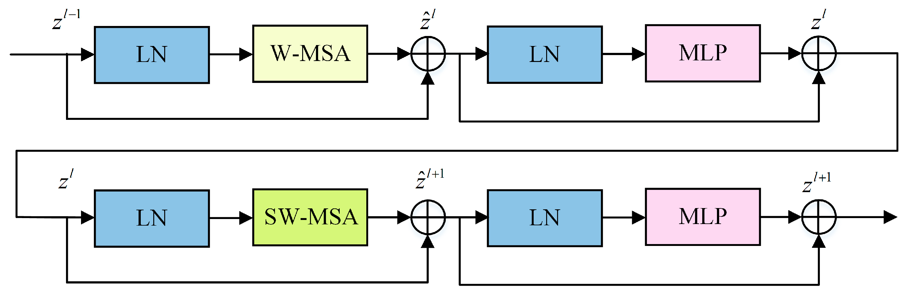
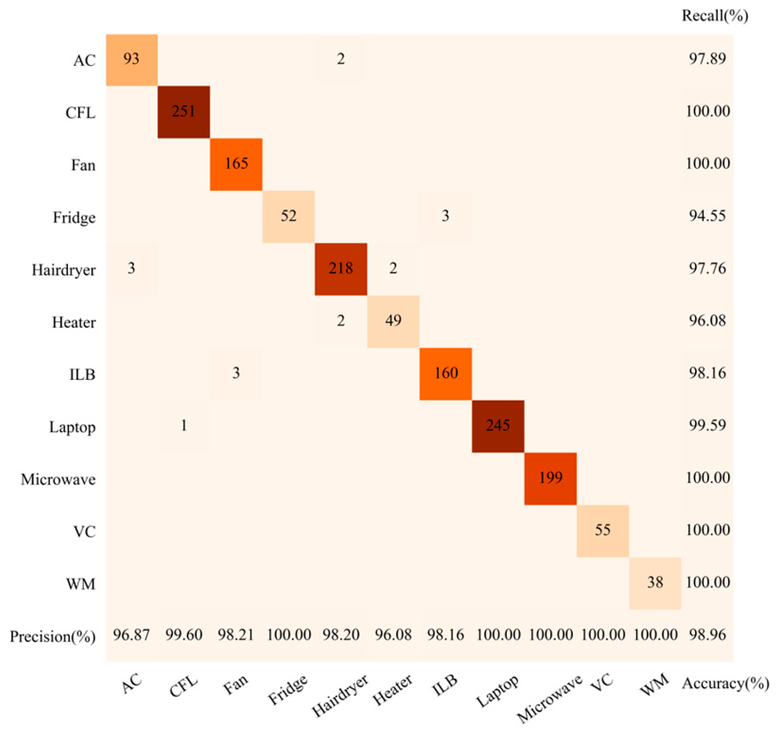
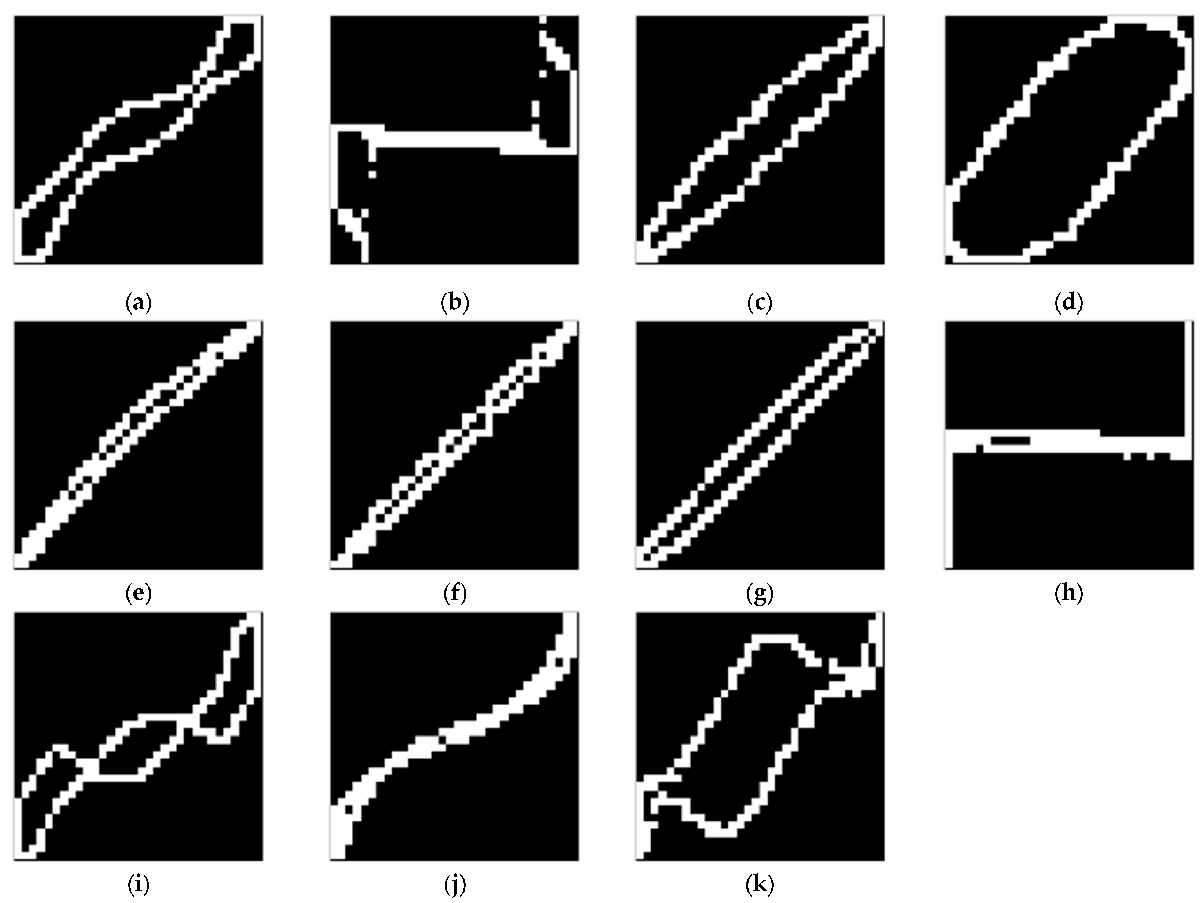
For two-dimensional image feature recognition, this paper adopts the Swin-Tiny (Swin-T) model, the variant with the lowest computational complexity within the Swin Transformer framework. The confusion matrix in Figure 10 shows the overall accuracy of 98.96%. The precision and recall rates for microwaves, vacuum cleaners, and washing machines all reach 100%. However, misclassifications occur for air conditioners, fridges, hairdryers, heaters, incandescent light bulbs, and laptops. By examining the binary V-I trajectory images in Figure 3, it can be observed that the fans, hairdryers, heaters, and incandescent light bulbs exhibit high trajectory similarity. Similarly, compact fluorescent lamps, and laptops also demonstrate close trajectory resemblance. Consequently, relying solely on two-dimensional binary V-I trajectory features proves insufficient for accurately distinguishing these appliances.

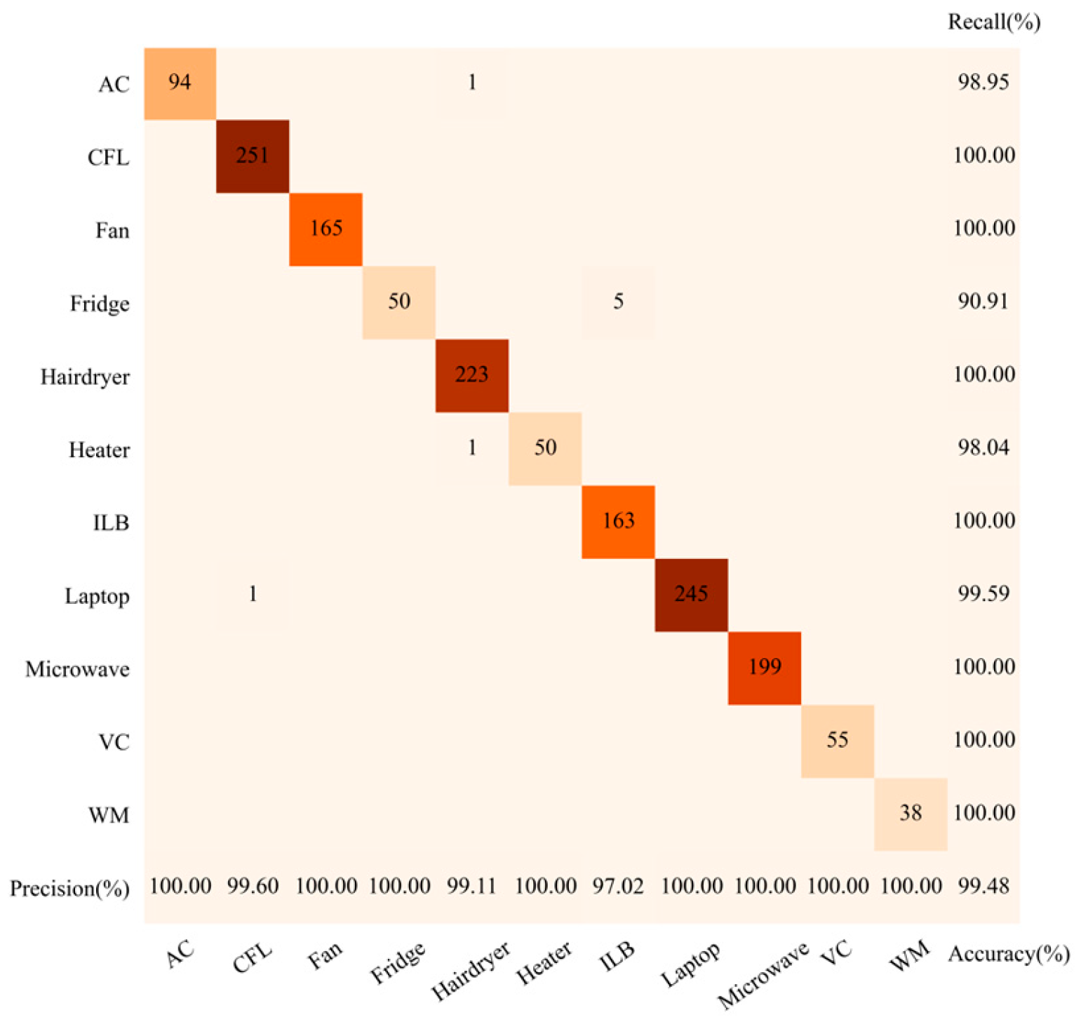
In Figure 11, the proposed method achieves the identification accuracy of 99.48% by combining one-dimensional numerical features and two-dimensional image features, with the recall rate of 90.91% for the fridges and precision/recall rates exceeding 97% for all other appliances. Notably, microwaves, vacuum cleaners, and washing machines are classified perfectly. Moreover, the fans are now fully and correctly identified, which are always prone to misclassification. Only a minimal number of air conditioners, fridges, heaters, and laptops remain misclassified.

A comparison of Figure 9e and Figure 10 reveals clear complementarity between the features of two dimensions. For instance, the air conditioners misclassified as the fans using numerical features are correctly identified when using image features; the hairdryers misclassified as the heaters based on image features are accurately recognized using numerical features. It is proved that the proposed method effectively makes use of the complementarity between multivariate features and significantly enhances the identification capability for multi-state loads.

This paper employs an information entropy-weighted ensemble method to integrate individual learners, achieving the fusion of one-dimensional numerical features (e.g., power and current) and two-dimensional binary V-I trajectory image features. To further validate the effectiveness of feature fusion, a comparative analysis is conducted with existing feature fusion methods from prior research, where the classification algorithms are replaced with Swin-T models, as shown in

Table 5. Comparison of different feature fusion methods.

Load Feature	Accuracy (%)	F-Score (%)	Runtime (min)
V-I trajectory + power [16]	93.83	93.80	168
Color Gram matrix [43]	98.21	98.19	121
Color V-I trajectory [17]	98.94	98.93	113
Enhanced color V-I trajectory [18]	99.17	99.15	126
The proposed method	99.48	99.47	105

.

As shown in Table 5, the method of reducing two-dimensional image features to one-dimensional numerical features through the neural network [16] not only results in lower accuracy but also requires the longest computation time. Although the approaches that convert all one-dimensional numerical features into two-dimensional image features [17,18,43] achieve some improvement in accuracy, their computation time remains higher than that of the method proposed in this paper due to the need for multiple operations on the image channels. Our method can more effectively leverage the quantitative statistical information of one-dimensional numerical features and the morphological information of two-dimensional image features without performing feature dimensionality transformation, making it more suitable for load identification scenarios involving feature fusion.

Table 6. Comparison of different deep network models.

Deep Network	Accuracy (%)	F-Score (%)	Runtime (min)
LeNet-5 [44]	90.50	90.46	21
AlexNet [17]	95.83	95.80	47
VGG-16 [45]	99.27	99.26	229
GoogLeNet [46]	97.32	97.31	78
ResNet-50 [47]	98.85	98.83	99
Swin-T	99.48	99.47	105

presents a comparison of the final results obtained by information entropy-weighted integration with other commonly used image recognition algorithms. It can be observed that the LeNet-5 algorithm model has the simplest network structure and the fewest parameters, but its recognition capability is too low. Compared to the LeNet-5 model, the AlexNet model increases the number of convolutional layers and the number of kernels per layer, resulting in improved accuracy, yet it still fails to meet the requirements for high-precision recognition. The VGG-16 model replaces single large convolutional kernels with cascaded small-sized kernels, achieving extremely high accuracy. However, due to a significant increase in parameters, its training time is more than twice that of Swin-T. The GoogleNet model and ResNet-50 model incorporate the InceptionV1 module and residual module, respectively, deepening the network layers. Although their computation time is slightly lower than Swin-T, they cannot match the classification performance of Swin-T. The adopted Swin-T model utilizes shifted windows and a self-attention mechanism, confining computations to local windows while capturing long-range dependencies in images, thereby achieving a balance between efficiency and performance.

As demonstrated in

Table 7. Comparison of different weighted ensemble methods.

Weight	Accuracy (%)	F-Score (%)	Runtime (min)
Equal weighting	98.70	98.68	104
Simple average weighting [38]	99.35	99.34	105
Accuracy-based weighting [48]	98.83	98.81	104
Ranking weighting [49]	99.22	99.21	105
Bayesian model averaging [50]	99.22	99.21	105
Information entropy weighting	99.48	99.47	105

, the experimental results show the following performance ranking: Information entropy weighting > Simple average weighting > Ranking weighting = Bayesian model averaging > Accuracy-based weighting > Equal weighting, while the runtime difference is negligible. This is because the information entropy-weighted ensemble method proposed in this paper fully accounts for the varying recognition performance of each classifier across different input samples. By leveraging the more accurate posterior probability information from classifier outputs to calculate entropy values, it adaptively assigns more reasonable fusion weights to different samples. Therefore, the proposed entropy-weighted ensemble approach achieves superior classification performance compared to alternative weighting strategies.

5.3.2. Results on the WHITED Dataset

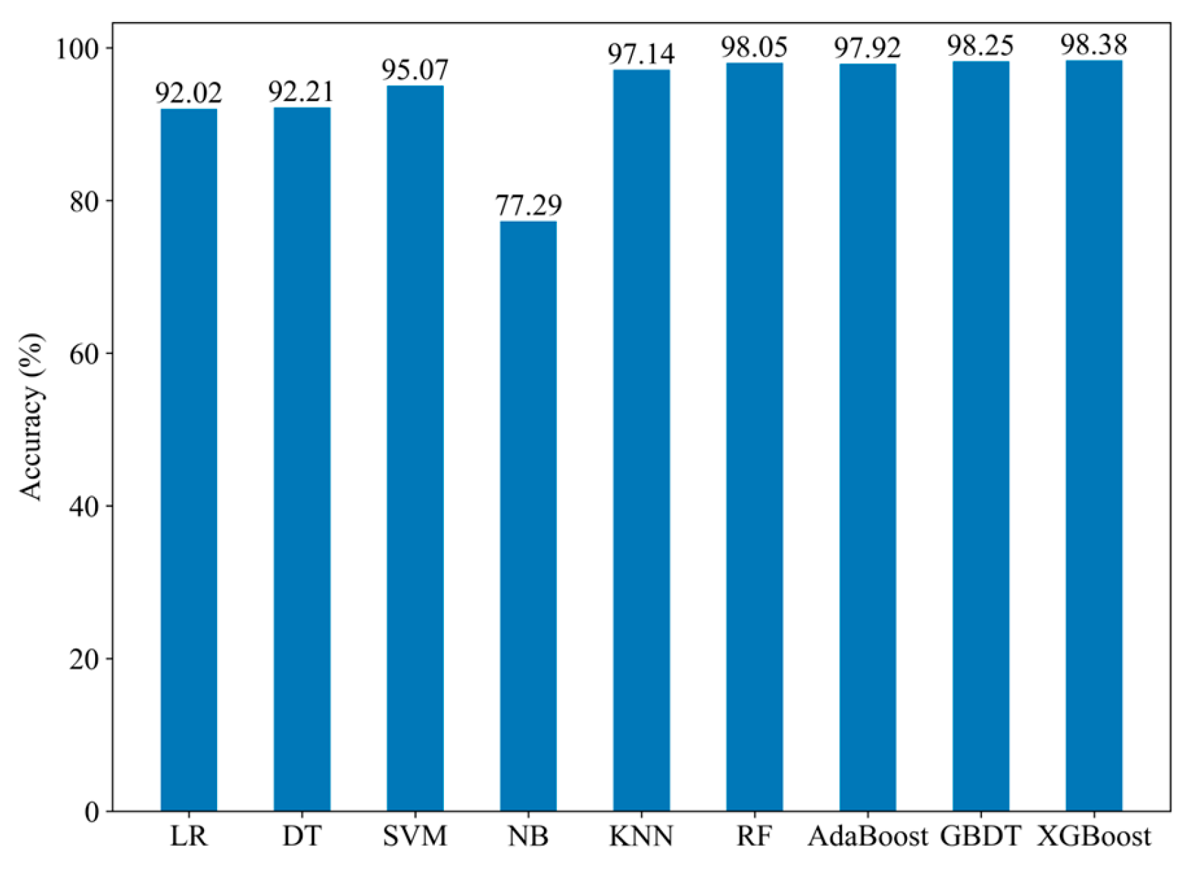
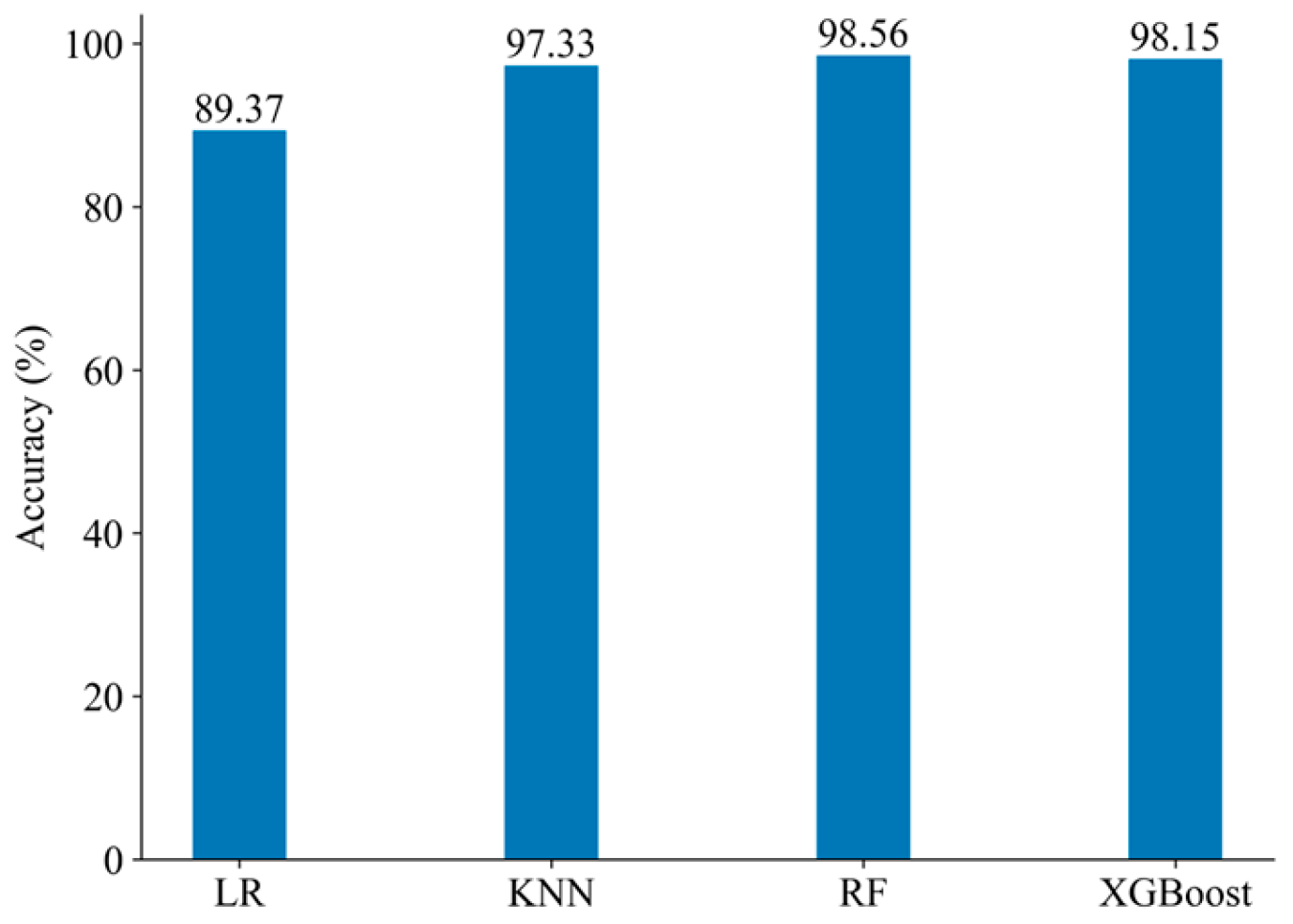
Following the same experimental procedure as that used with the PLAID dataset, the base learners selected for the WHITED dataset based on diversity metrics and accuracy indicators are LR, KNN, RF, and XGBoost. The accuracy of each base learner is shown in Figure 12.

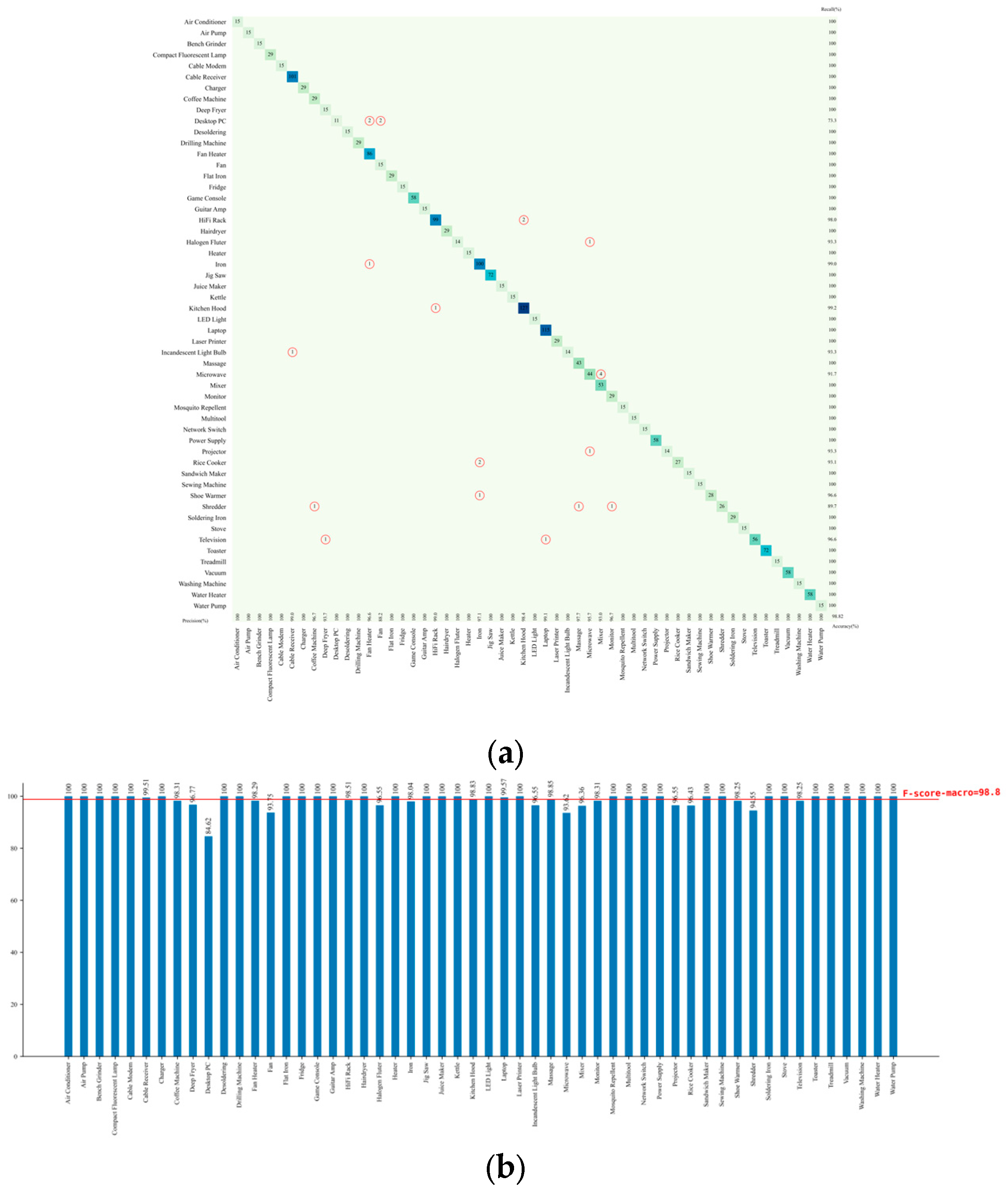
The classification results obtained by combining the four base learners using information entropy-weighted ensemble learning are shown in Figure 12. The proposed load identification method, using one-dimensional numerical features, still performs well on the WHITED dataset. It achieves an overall accuracy of 98.82% and an F-score of 98.8%.

As shown in Figure 13, the identification performance for laptops is relatively lower, primarily due to confusion with two other types of appliances: fans and fan heaters. The power characteristics of laptops exhibit significant fluctuations with changes of load. Similarly, fans experience power fluctuations due to speed adjustments or variations in natural airflow, while fan heaters exhibit intermittent on-off behavior as a result of temperature control regulation. These similar dynamic characteristics lead to overlapping steady states in one-dimensional numerical features. Therefore, it is necessary to incorporate higher-dimensional features to further enhance the ability to distinguish multi-state appliances.

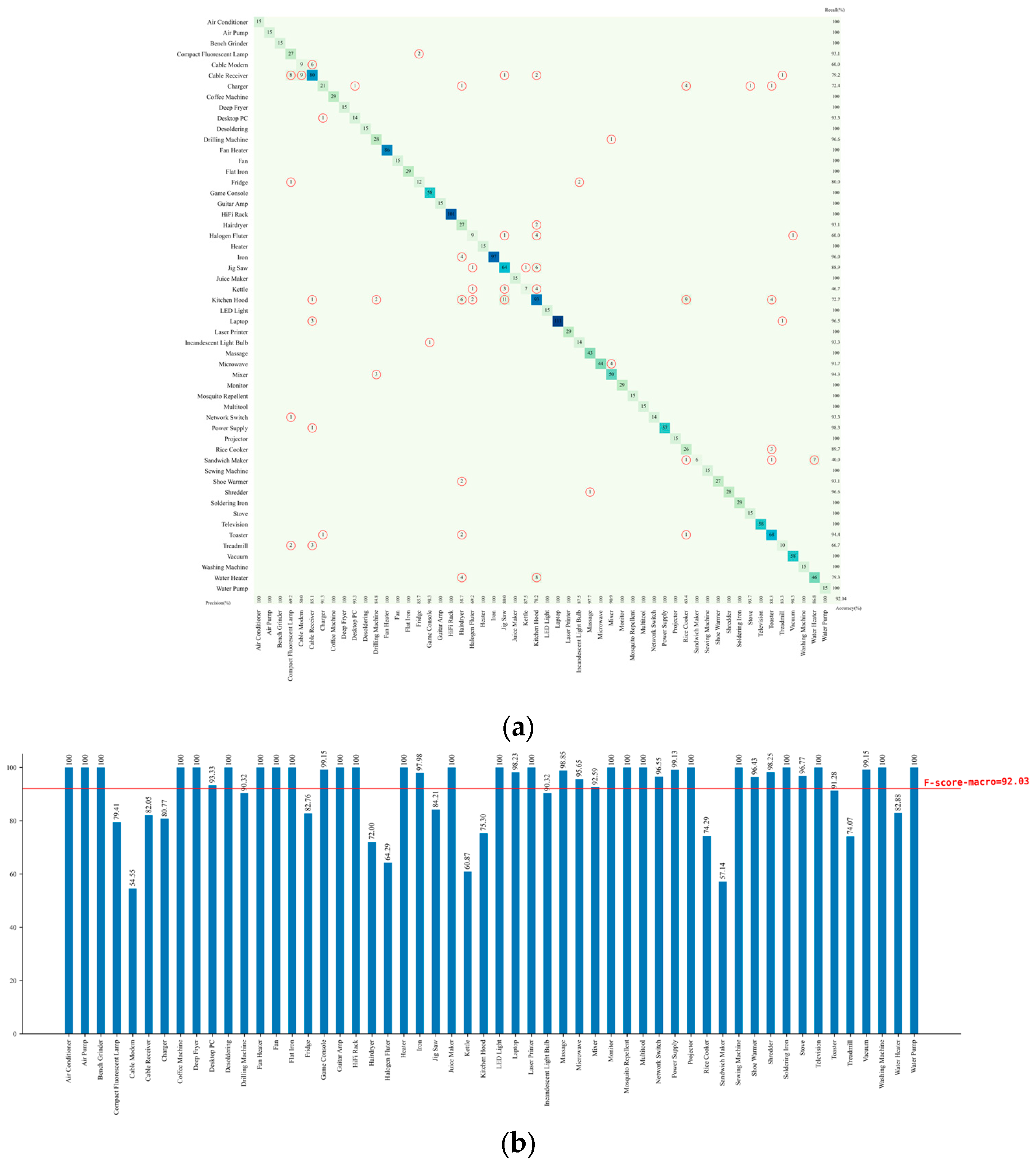
Figure 14 demonstrates the identification results of two-dimensional image features on the WHITED dataset using Swin-T. The model achieved an accuracy of 92.04% and an F-score of 92.03%. Appliances such as cable modems, halogen fluters, kettles, and sandwich makers exhibited significantly lower F-scores than the average, indicating that classification models based solely on two-dimensional binary V-I trajectory images still face certain limitations in accurately identifying these types of appliances.

The overall accuracy of identifying appliances using two-dimensional image features on the WHITED dataset is relatively lower compared to the PLAID dataset. This is because the PLAID dataset contains only 11 types of appliances, whereas the WHITED dataset includes a much richer set of 54 appliance types. As the number of appliance categories increases, the probability of different appliances exhibiting similar V-I trajectory shapes becomes higher, making it more difficult for deep neural networks to effectively capture subtle distinctions.

As illustrated in Figure 15, the proposed load identification method based on multivariate features and information entropy-weighted ensemble also meets the high accuracy requirements on the WHITED dataset. The experimental results demonstrate that the overall accuracy and F-score on the WHITED dataset both reach 99.54%. Among the tested appliance categories, only a few misclassifications occurred for halogen fluters, kitchen hoods, microwaves, shoe warmers, and shredders, while the identification accuracy for all other appliances reached 100%. Compared to the method using only one-dimensional numerical features, the proposed method improves the accuracy and F-score by 0.72% and 0.74%, respectively. When compared to the method relying solely on two-dimensional image features, the improvements are even more significant, reaching 7.5% and 7.51%, respectively.

By comparing the classification results on the PLAID and WHITED datasets, it is observed that the proposed method demonstrates strong cross-dataset adaptability. In tests on both datasets, the F-scores for all appliance categories consistently remained above 94%, reflecting a high level of performance. These experimental results provide strong evidence that the proposed multivariate feature fusion strategy, based on the collaboration of multiple classifiers, offers significant advantages over traditional single-dimensional feature methods. It effectively addresses scenarios involving a large variety of appliance types and multiple brands within the same appliance category.

In summary, it can be observed that the appliances with remaining classification errors are mainly multi-state devices in both the PLAID and WHITED datasets. These devices typically operate cyclically or intermittently, and during different steady operating states, power values are similar while V-I trajectory shapes are also alike. Therefore, future research could consider incorporating transient features, such as startup current pulse amplitude, transient response time, and instantaneous power change rate. Fusing them with steady-state features may enhance the clarity of classifier decision boundaries.

6. Conclusions

This paper proposes a non-intrusive load identification method based on multivariate features and information entropy-weighted ensemble. Separate processing modules are established for one-dimensional numerical features and two-dimensional image features. Information entropy is employed to adaptively determine the weights of each classifier, and a weighted voting strategy is used to obtain the final identification result. This approach holds significant implications for the development of the NILM field:

• It improves the accuracy of non-intrusive load identification, making it applicable to scenarios requiring fine-grained load recognition, such as smart homes and energy management systems. Users can obtain more precise identification of their electrical appliances, aiding in optimizing electricity usage behaviors. Meanwhile, power grids can acquire critical data for refined demand-side management and provide users with personalized energy-saving recommendations.
• It verifies the effectiveness of a hybrid modular architecture combining traditional machine learning and deep learning in non-intrusive load identification, offering a new paradigm for future research. Each module can be independently optimized and updated, which provides important reference value for edge computing scenarios, such as deployment on embedded devices.
• It enhances the interpretability of non-intrusive load identification models. The information entropy-weighted voting mechanism offers an intuitive measure of classification confidence. By reducing the voting weight of classifiers with higher entropy on specific samples, the method effectively mitigates the influence of unreliable information, thereby aiding anomaly detection and model diagnostics.

However, the proposed model still faces multiple challenges in practical deployment and application, which need to be addressed in future research:

• In learner selection based on diversity metrics, it is necessary to develop a dynamic or adaptive thresholding strategy to determine the acceptable range of diversity metrics, thereby maximizing load identification accuracy.
• Deep learning networks often require retraining from scratch when applied to new target domains. Future work could explore the use of transfer learning, whereby models are pre-trained on large-scale public datasets and subsequently adapted to target scenarios, significantly reducing the computational cost of training.
• Although the method achieves a high level of discrimination among household appliance loads, it has not yet reached 100% accuracy, and its applicability in commercial or industrial production environments remains limited. Further improvements to load identification models are needed to meet the demands of more complex scenarios.

References

1. Gopinath, R.; Kumar, M.; Joshua, C.P.C.; Srinivas, K. Energy Management Using Non-Intrusive Load Monitoring Techniques—State-of-the-Art and Future Research Directions. Sustain. Cities Soc. 2020, 62, 102411. [Google Scholar] [CrossRef]
2. Dinesh, C.; Nettasinghe, B.W.; Godaliyadda, R.I.; Ekanayake, M.P.B.; Ekanayake, J.; Wijayakulasooriya, J.V. Residential Appliance Identification Based on Spectral Information of Low Frequency Smart Meter Measurements. IEEE Trans. Smart Grid 2015, 7, 2781–2792. [Google Scholar] [CrossRef]
3. Luan, W.; Yang, F.; Zhao, B.; Liu, B. Industrial Load Disaggregation Based on Hidden Markov Models. Electr. Power Syst. Res. 2022, 210, 108086. [Google Scholar] [CrossRef]
4. Figueiredo, M.; De Almeida, A.; Ribeiro, B. Home Electrical Signal Disaggregation for Non-Intrusive Load Monitoring (NILM) Systems. Neurocomputing 2012, 96, 66–73. [Google Scholar] [CrossRef]
5. Yuan, J.; Wang, H.; Wu, P.; Wang, C.; Chen, J.; Jiao, H. A Novel Current Signal Feature and Its Application in Noninvasive Load Monitoring. IEEE Trans. Instrum. Meas. 2020, 70, 1–10. [Google Scholar] [CrossRef]
6. Bouhouras, A.S.; Gkaidatzis, P.A.; Panagiotou, E.; Hatziargyriou, N.D. A NILM algorithm with enhanced disaggregation scheme under harmonic current vectors. Energy Build. 2019, 183, 392–407. [Google Scholar] [CrossRef]
7. Yang, D.; Kong, L.; Hu, B.; Yuan, T. Load Identification Method Based on Multi-Feature Sequence Fusion. Autom. Electr. Power Syst. 2017, 41, 66–73. [Google Scholar]
8. Qi, B.; Dong, C.; Wu, X.; Cui, G. Non-Intrusive Load Identification Method Based on DTW Algorithm and Steady-State Current Waveform. Autom. Electr. Power Syst. 2018, 42, 70–76. [Google Scholar]
9. Bouhouras, A.S.; Gkaidatzis, P.A.; Chatzisavvas, K.C.; Panagiotou, E.; Poulakis, N.; Christoforidis, G.C. Load Signature Formulation for Non-Intrusive Load Monitoring Based on Current Measurements. Energies 2017, 10, 538. [Google Scholar] [CrossRef]
10. Sun, Y.; Cui, C.; Lu, J.; Hao, J.; Liu, X. Non-Intrusive Load Monitoring Method Based on Delta Feature Extraction and Fuzzy Clustering. Autom. Electr. Power Syst. 2017, 41, 86–91. [Google Scholar]
11. Matindife, L.; Sun, Y.; Wang, Z. Image-based mains signal disaggregation and load recognition. Complex Intell. Syst. 2021, 7, 901–927. [Google Scholar] [CrossRef]
12. Li, J.; Liu, Y.; Zhou, L.; Deng, H. Research on Electric Load Identification Method of Integrated Energy System Based on Image Analysis. In Proceedings of the 2023 IEEE 3rd International Conference on Electronic Technology, Communication and Information (ICETCI), Shijiazhuang, China, 15–17 September 2023; IEEE: Piscataway, NJ, USA, 2023; pp. 484–489. [Google Scholar]
13. Cavalca, D.L.; Fernandes, R.A.S. Recurrence plots and convolutional neural networks applied to nonintrusive load monitoring. In Proceedings of the 2020 IEEE Power & Energy Society General Meeting (PESGM), Virtual Conference, 3–6 August 2020; IEEE: Piscataway, NJ, USA, 2020; pp. 1–5. [Google Scholar]
14. Baptista, D.; Mostafa, S.S.; Pereira, L.; Melício, R. Implementation strategy of convolution neural networks on field programmable gate arrays for appliance classification using the voltage and current (VI) trajectory. Energies 2018, 11, 2460. [Google Scholar] [CrossRef]
15. De Baets, L.; Develder, C.; Dhaene, T.; Deschrijver, D. Detection of unidentified appliances in non-intrusive load monitoring using siamese neural networks. Int. J. Electr. Power Energy Syst. 2019, 104, 645–653. [Google Scholar] [CrossRef]
16. Wang, S.X.; Guo, L.Y.; Chen, H.; Deng, X.Y. Non-Intrusive Load Identification Algorithm Based on Feature Fusion and Deep Learning. Autom. Electr. Power Syst. 2020, 44, 103–110. [Google Scholar]
17. Liu, Y.; Wang, X.; You, W. Non-Intrusive Load Monitoring by Voltage–Current Trajectory Enabled Transfer Learning. IEEE Trans. Smart Grid 2018, 10, 5609–5619. [Google Scholar] [CrossRef]
18. Wang, S.; Chen, H.; Guo, L.; Xu, D. Non-Intrusive Load Identification Based on the Improved Voltage-Current Trajectory with Discrete Color Encoding Background and Deep-Forest Classifier. Energy Build. 2021, 244, 111043. [Google Scholar] [CrossRef]
19. Medico, R.; De Baets, L.; Gao, J.; Giri, S.; Kara, E.; Dhaene, T.; Develder, C.; Bergés, M.; Deschrijver, D. A Voltage and Current Measurement Dataset for Plug Load Appliance Identification in Households. Sci. Data 2020, 7, 49. [Google Scholar] [CrossRef]
20. Kahl, M.; Haq, A.U.; Kriechbaumer, T.; Jacobsen, H.A. WHITED—A worldwide household and industry transient energy data set. In Proceedings of the 3rd International Workshop on Non-Intrusive Load Monitoring (NILM), Vancouver, BC, Canada, 14–15 May 2016; pp. 1–4. [Google Scholar]
21. Wang, P.; Geng, L.; Liu, X.; Cheng, H.; Fang, K.; Zhang, X. Non-Intrusive Load Feature Extraction Method Based on Online Feature Library. Proc. CSEE 2024, 44, 3489–3500. [Google Scholar]
22. Lam, H.Y.; Fung, G.S.K.; Lee, W.K. A Novel Method to Construct Taxonomy Electrical Appliances Based on Load Signatures. IEEE Trans. Consum. Electron. 2007, 53, 653–660. [Google Scholar] [CrossRef]
23. Shabbir, N.; Vassiljeva, K.; Hokmabad, H.N.; Husev, O.; Petlenkov, E.; Belikov, J. Comparative Analysis of Machine Learning Techniques for Non-Intrusive Load Monitoring. Electronics 2024, 13, 1420. [Google Scholar] [CrossRef]
24. Mollel, R.S.; Stankovic, L.; Stankovic, V. Explainability-Informed Feature Selection and Performance Prediction for Nonintrusive Load Monitoring. Sensors 2023, 23, 4845. [Google Scholar] [CrossRef] [PubMed]
25. Zhou, Y.; Zhang, S.; Ran, B.; Yang, W.; Wang, Y.; Xiao, X. Event-Based Two-Stage Non-Intrusive Load Monitoring Method Involving Multi-Dimensional Features. CSEE J. Power Energy Syst. 2022, 9, 1119–1128. [Google Scholar]
26. Yang, C.C.; Soh, C.S.; Yap, V.V. A Non-Intrusive Appliance Load Monitoring for Efficient Energy Consumption Based on Naive Bayes Classifier. Sustain. Comput. Inform. Syst. 2017, 14, 34–42. [Google Scholar] [CrossRef]
27. Jaramillo, A.F.M.; Lopez-Lorente, J.; Laverty, D.M.; Brogan, P.V.; Hoyos Velasquez, S.H.; Martinez-Del-Rincón, J. Distributed Energy Resources Electric Profile Identification in Low Voltage Networks Using Supervised Machine Learning Techniques. IEEE Access 2023, 11, 19469–19486. [Google Scholar] [CrossRef]
28. Wu, X.; Gao, Y.; Jiao, D. Multi-Label Classification Based on Random Forest Algorithm for Non-Intrusive Load Monitoring System. Processes 2019, 7, 337. [Google Scholar] [CrossRef]
29. Ullah, A.; Javaid, N.; Asif, M.; Javed, M.U.; Yahaya, A.S. AlexNet, AdaBoost and Artificial Bee Colony Based Hybrid Model for Electricity Theft Detection in Smart Grids. IEEE Access 2022, 10, 18681–18694. [Google Scholar] [CrossRef]
30. Zhang, C.; Liu, C.; Zhang, X.; Almpanidis, G. An Up-to-Date Comparison of State-of-the-Art Classification Algorithms. Expert Syst. Appl. 2017, 82, 128–150. [Google Scholar] [CrossRef]
31. Chen, Z.; Chen, J.; Xu, X.; Peng, S.; Xiao, J.; Qiao, H. Non-Intrusive Load Monitoring Based on Feature Extraction of Change-Point and XGBoost Classifier. In Proceedings of the 2020 IEEE 4th Conference on Energy Internet and Energy System Integration (EI2), Wuhan, China, 30 October–1 November 2020; IEEE: Piscataway, NJ, USA, 2020; pp. 2652–2656. [Google Scholar]
32. Sadeghianpourhamami, N.; Ruyssinck, J.; Deschrijver, D.; Dhaene, T.; Develder, C. Comprehensive Feature Selection for Appliance Classification in NILM. Energy Build. 2017, 151, 98–106. [Google Scholar] [CrossRef]
33. Gregorutti, B.; Michel, B.; Saint-Pierre, P. Correlation and Variable Importance in Random Forests. Stat. Comput. 2017, 27, 659–678. [Google Scholar] [CrossRef]
34. Sun, B.; Wang, J.; Chen, H.; Wang, Y. Diversity Measures in Ensemble Learning. Control Decis. 2014, 29, 385–395. [Google Scholar]
35. Liu, Z.; Lin, Y.; Cao, Y.; Hu, H.; Wei, Y.; Zhang, Z.; Lin, S.; Guo, B. Swin Transformer: Hierarchical Vision Transformer Using Shifted Windows. In Proceedings of the IEEE/CVF International Conference on Computer Vision, Montreal, BC, Canada, 11–17 October 2021; pp. 10012–10022. [Google Scholar]
36. Dosovitskiy, A.; Beyer, L.; Kolesnikov, A.; Weissenborn, D.; Zhai, X.; Unterthiner, T.; Dehghani, M.; Minderer, M.; Heigold, G.; Gelly, S.; et al. An Image is Worth 16x16 Words: Transformers for Image Recognition at Scale. arXiv 2020, arXiv:2010.11929. [Google Scholar]
37. Ghosh, S.; Mitra, A.; Chakrabarti, S.; Sharma, A. Data-Driven Strategy for Appliance Identification Using Phase-Space Reconstruction. IEEE Trans. Smart Grid 2023, 14, 4964–4967. [Google Scholar] [CrossRef]
38. Zhou, Z.H. Machine Learning; Tsinghua University Press: Beijing, China, 2016; pp. 33–35, 171–173. [Google Scholar]
39. Pereira, L.; Nunes, N. Performance Evaluation in Non-Intrusive Load Monitoring: Datasets, Metrics, and Tools—A Review. Wiley Interdiscip. Rev. Data Min. Knowl. Discov. 2018, 8, e1265. [Google Scholar] [CrossRef]
40. De Baets, L.; Ruyssinck, J.; Develder, C.; Dhaene, T.; Deschrijver, D. Appliance Classification Using VI Trajectories and Convolutional Neural Networks. Energy Build. 2018, 158, 32–36. [Google Scholar] [CrossRef]
41. Kang, H.; Kim, H. Household Appliance Classification Using Lower Odd-Numbered Harmonics and the Bagging Decision Tree. IEEE Access 2020, 8, 55937–55952. [Google Scholar]
42. Wang, L.; Ma, J.; Han, X.; Xue, S.; Yang, R.; Bai, H. Non-Intrusive Load Monitoring Method With Multi-State Characterization of Loads. Power Syst. Technol. 2024, 48, 4720–4728. [Google Scholar]
43. Chen, J.; Wang, X.; Zhang, H. Non-Intrusive Load Recognition Using Color Encoding in Edge Computing. Chin. J. Sci. Instrum. 2020, 41, 12–19. [Google Scholar]
44. Tian, S.; Zhang, J.; Shu, X.; Chen, L.; Niu, X.; Wang, Y. A Novel Evaluation Strategy to Artificial Neural Network Model Based on Bionics. J. Bionic Eng. 2022, 19, 1–16. [Google Scholar] [CrossRef]
45. Moreno, S.; Teran, H.; Villarreal, R.; Vega-Sampayo, Y.; Paez, J.; Ochoa, C.; Espejo, C.A.; Chamorro-Solano, S.; Montoya, C. An Ensemble Method for Non-Intrusive Load Monitoring (NILM) Applied to Deep Learning Approaches. Energies 2024, 17, 4548. [Google Scholar] [CrossRef]
46. Hua, C.; Chen, S.; Xu, G.; Lu, Y.; Du, B. Defect Identification Method of Carbon Fiber Sucker Rod Based on GoogLeNet-Based Deep Learning Model and Transfer Learning. Mater. Today Commun. 2022, 33, 104228. [Google Scholar] [CrossRef]
47. Zhang, Y.; Qian, W.; Ye, Y.; Li, Y.; Tang, Y.; Long, Y.; Duan, M. A Novel Non-Intrusive Load Monitoring Method Based on ResNet-seq2seq Networks for Energy Disaggregation of Distributed Energy Resources Integrated with Residential Houses. Appl. Energy 2023, 349, 121703. [Google Scholar] [CrossRef]
48. Jiangzhou, C.; Xie, S.; Zhang, Y. Non-Invasive Load Identification Based on Clustering Weighted Random Forest. Smart Power 2020, 48, 123–129. [Google Scholar]
49. Wijaya, D.R.; Afianti, F. Information-Theoretic Ensemble Feature Selection with Multi-Stage Aggregation for Sensor Array Optimization. IEEE Sens. J. 2020, 21, 476–489. [Google Scholar] [CrossRef]
50. Zhou, Z.H. Ensemble Methods: Foundations and Algorithms; CRC Press: Boca Raton, FL, USA, 2012; pp. 74–75. [Google Scholar]
Figure 1. The framework of the NILM process is based on multivariate features and an information entropy-weighted ensemble.
Energies 18 02369 g001
Figure 2. Collected data of incandescent light bulbs in the PLAID dataset: (a) Voltage waveform; (b) Current waveform.
Energies 18 02369 g002
Figure 3. The binary V-I trajectory images (q = 32) of 11 appliances from the PLAID dataset: (a) Air Conditioner (AC); (b) Compact Fluorescent Lamp (CFL); (c) Fan; (d) Fridge; (e) Hairdryer; (f) Heater; (g) Incandescent Light Bulb (ILB); (h) Laptop; (i) Microwave; (j) Vacuum Cleaner (VC); (k) Washing Machine (WM).
Energies 18 02369 g003
Figure 4. The overall architecture of the Swin Transformer.
Energies 18 02369 g004
Figure 5. The architecture of the Swin Transformer block.
Energies 18 02369 g005
Figure 6. Current harmonic amplitude of appliances: (a) Compact Fluorescent Lamp; (b) Hairdryer; (c) Microwave.
Energies 18 02369 g006
Figure 7. Diversity measure of nine learners: (a) Q-statistic; (b) DF.
Energies 18 02369 g007
Figure 8. Accuracy rate of nine learners.
Energies 18 02369 g008
Figure 9. Confusion matrix of the preliminary identification results for one-dimensional numerical features: (a) LR; (b) KNN; (c) Adaboost; (d) GBDT; (e) Four learners combined by information entropy-weighted ensemble method. (Darker colors represent larger quantities).
Energies 18 02369 g009aEnergies 18 02369 g009b
Figure 10. Confusion matrix of the preliminary identification results for two-dimensional image features. (Darker colors represent larger quantities).
Energies 18 02369 g010
Figure 11. Confusion matrix of final classification results combining one-dimensional numerical features and two-dimensional image features. (Darker colors represent larger quantities).
Energies 18 02369 g011
Figure 12. Accuracy rate of individual learners on the WHITED dataset.
Energies 18 02369 g012
Figure 13. Preliminary identification results for one-dimensional numerical features on the WHITED dataset: (a) Confusion matrix (Darker colors represent larger quantities); (b) F-score.
Energies 18 02369 g013
Figure 14. Preliminary identification results for two-dimensional image features on the WHITED dataset: (a) Confusion matrix (Darker colors represent larger quantities); (b) F-score.
Energies 18 02369 g014
Figure 15. Multivariate feature identification results on the WHITED dataset: (a) Confusion matrix (Darker colors represent larger quantities); (b) F-score.
Energies 18 02369 g015