Article

Modeling Retail Buildings Within Renewable Energy Communities: Generation and Implementation of Reference Energy Use Profiles

by
Samuele Lozza
1,
Matteo Caldera
2,
Daniele Fava
2,
Martina Ferrando
1 and
Francesco Causone
1,*
1
Department of Energy, Politecnico di Milano, Via Lambruschini 4, 20156 Milano, Italy
2
Department of Energy Technologies and Renewable Sources, Italian National Agency for New Technologies Energy and Sustainable Economic Development (ENEA), Via Stezzano 87, 24126 Bergamo, Italy
*
Author to whom correspondence should be addressed.
Energies 2025, 18(9), 2368; https://doi.org/10.3390/en18092368
Submission received: 31 March 2025 / Revised: 14 April 2025 / Accepted: 15 April 2025 / Published: 6 May 2025

Abstract

:
In a constantly evolving context where non-dispatchable renewable energy sources (RESs) are becoming increasingly widespread, the role of Renewable Energy Communities (RECs) is gaining momentum as a way to promote distributed self-consumption. The spreading of RECs in the European Union (EU) has been supported by the development of technical tools. RECON (Renewable Energy Community ecONomic simulator) is one the most used simulation tools for energy, economic, and financial pre-assessments of RECs in Italy. This software requires, as an input to simulation, the electrical energy use profiles of buildings to estimate the shared energy and, consequently, to calculate economic incentives. However, the availability of reference electrical energy use profiles remains limited, especially when it comes to specific uses such as for organized large-scale retail. To address this issue, this study developed a data-driven model capable of generating electrical energy use profiles specific for organized large-scale retail, using a limited number of inputs, and thereby, addressing the gap in current energy modeling practices. The model validation showed that the model replicates electric energy profiles, on an annual basis, with an average deviation below 5% using minimal inputs. Monthly simulations exhibit greater discrepancies during colder months, which suggest further refinement opportunities.

1. Introduction

The continuous increase in electric energy demand and the willingness to adopt renewable solutions to counteract climate change has led the European Union (EU) to set ambitious objectives in this regard, such as becoming the first climate-neutral continent by 2050 [1], which is at the heart of the European Green Deal [2].
To achieve this, the EU has undertaken different initiatives to transition towards a distributed generation and renewable energy system, which boosted, over the years, the share of renewable energy sources (RESs) in the generation of electricity [3,4].
One of these initiatives is the introduction, in 2018, of the Renewable Energy Directive II (RED II) [5], which set a goal to raise the share of energy from renewable sources in the Union’s gross final consumption to 32% by 2030 (lately further increased to 42.5% [6]). It also introduced the concept of Renewable Energy Communities (RECs), i.e., a legal entity composed of citizens, local businesses, public entities, and organizations that produce and share renewable electricity from community-affiliated RES installations using the national grid for virtual energy exchange, thereby evolving the role of the citizen from being a passive consumer to an active participant in the energy market [7,8].
RECs are emerging initiatives with the potential to transform the relationships between end-users and other actors in the energy sector. By collectively investing in the production, sale, distribution, and consumption of renewable energy, participants engage in the energy transition and generate a series of benefits. These include mitigating climate change, stimulating the local economy, mitigating energy poverty, and promoting stakeholder engagement, while also reducing energy bills for members and creating new funding opportunities for local initiatives [9,10,11,12].
Furthermore, citizens are not the only ones who can participate in RECs; small and medium enterprises (SMEs) can also be a part of them, as long as their participation does not constitute their main source of income. In analogy to this, as observed by E. Veronese et al. [13]:
“Industrial and commercial users may take the lead in the spread of these types of configuration, leveraging their remarkable prospect of capital investment.”
Despite these opportunities, RECs remain a relatively new model for energy production and sharing [14]. In particular, the participation of Organized Large-Scale Retail (OLSR), classified as SMEs, is a topic that is still unexplored in the RECs’ literature.
In this context, various simulation tools have been developed to model RECs [15,16,17,18]. Notably, RECON (Renewable Energy Community ecONomic simulator) [15] by ENEA, the Italian National Agency for New Technologies, Energy and Sustainable Development, represents one of such tools. However, a significant limitation of these tools is their reliance on electric energy (EE) use profiles, which can be challenging to obtain [19]. Electric energy use profiles are necessary to simulate diffuse self-consumption configurations, as their absence would prevent accurate calculations of the energy consumed and shared within REC configurations [20,21]. In fact, the calculations are based on an hourly energy balance, a method that is crucial for technical accuracy and, according to the Italian transposition of the RED II directive, carries significant economic consequences [14,22].
In order to develop electric energy use profiles, two fundamental approaches can be generally employed: engineering-based (or physics-based) modeling and data-driven modeling. The physics-based model employs advanced high-resolution engineering techniques that simulate energy demand based on the building’s thermal, energy, and architectural characteristics, whereas data-driven approaches directly model the building’s energy performance using statistical methods. A possible way to classify data-driven techniques for energy demand prediction includes: conventional statistical methods, classification-based models, support vector regression (SVR), artificial neural networks (ANN), genetic algorithms, and grey and fuzzy models [23,24,25,26,27].
It is also worth noting that various techniques exist for generating electric energy use profiles. These range from traditional statistical approaches to advanced machine learning methods. Machine learning algorithms, in particular, offer significant advantages in terms of forecasting and adaptability, enabling the generation of more accurate and customizable profiles [28,29,30].
Numerous studies has addressed the generation of electric consumption profiles [31,32,33,34]. In particular, for applications to retail buildings, Rana et al. [35] proposed a comprehensive investigation into the load contributions attributable to air conditioning systems. Moreover, significant attention has been devoted to developing accurate consumption profiles. With regard to the generation of profiles for OLSR, two studies (Granell et al. [36] and M. Orr [37]) have utilized these techniques.
Granell et al. [36] proposed a data-driven method that, given a time interval, calculates the average energy value and the slope of the line connecting the initial and final energy values. The energy profile is characterized by eight elements: four key periods, the average consumption during off-peak and peak periods, and the slopes during the transients, which indicate an increase and a decrease in demand, respectively. By using this information, the estimated profile is geometrically reconstructed by assigning the average values to the off-peak and peak periods and modeling the transitions with linear segments.
On the other hand, M. Orr [37] focused on deep learning models, particularly Convolutional Neural Networks (CNN), which have proven effective in enhancing electricity demand forecasting. These models can capture complex, non-linear relationships between variables, which is a crucial feature for accurate energy consumption prediction. Moreover, Orr’s study examines whether incorporating forecasted weather data can improve forecasting accuracy by comparing predictions based on historical versus forecasted weather data.
While the literature abounds with studies on the modeling of EE use profiles for buildings, especially in the residential sector [38,39,40,41,42], many of these models are not directly applicable to other building types due to the large difference in electric energy consumption and end-user EE profiles [43,44]. In particular, there is a scarcity of research focused on electric energy use profiles for OLSR, that, as explained before, may play a relevant role in RECs diffusion. Recognizing this gap and given the limited amount of available data, which does not justify the use of advanced algorithms designed for large databases, this study focuses on developing a data-driven model, inspired by the methodology proposed by Granell et al. [36] to generate accurate and customizable OLSR energy use profiles’ using only minimal input data. The developed model has been integrated in RECON beta testing environment to allow simulations that improve the potential of RECs assessment in Italy.
The main contributions of the study include the implementation of an innovative methodology that bridges the gaps in current energy modeling practices, its integration into the RECON beta testing environment, and the generation of new knowledge through validation against real data.

2. Materials and Methods

The following chapter is divided into three sections:
  • EE use profile generation from the exiting database;
  • Integration of the EE use profile in the RECON beta testing environment;
  • Model validation.
Section 2 is dedicated to the development of the model, which was specifically designed for implementation within the RECON beta testing environment. The developed model is based on the profiles generated in Section 1; given that these consumption profiles are derived from raw data datasets, the model has been classified as data-driven.
All the tasks have been performed in the numerical computing environment of Matlab R2024b [45].

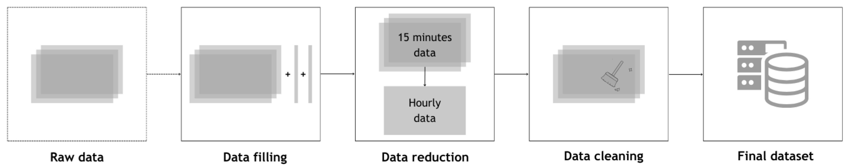
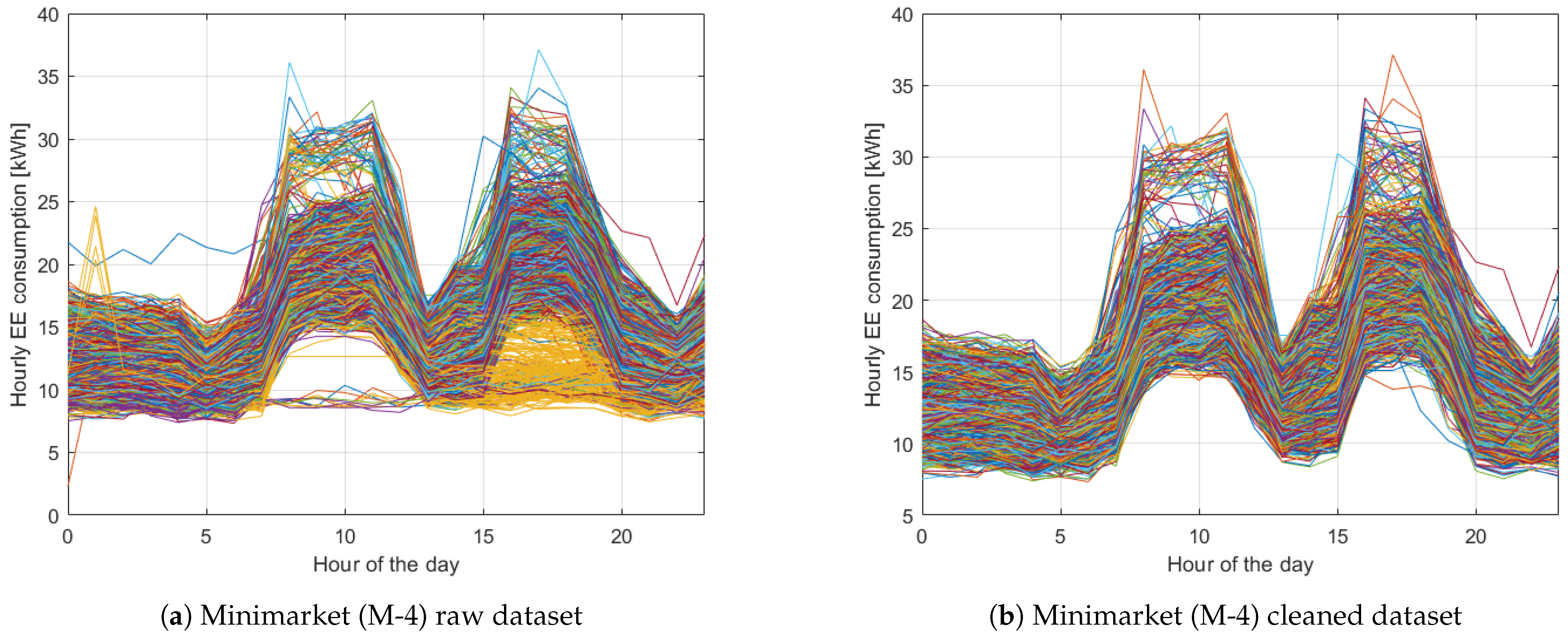
2.1. EE Use Profile Generation from Exiting Database

To create an EE use profile, it is necessary to rely on hourly or quarter-hourly electricity consumption data. For the purpose of this study, a database made of hourly or quarter-hourly electricity net meter readings (which follow the Measuring Instruments Directive 2014/32/EU [46]), from year 2021 to year 2024 for seven buildings, was available, which is reported in Table 1.
The OLSRs reported in Table 1 have been divided in two categories: minimarket and superstore. The minimarket is characterized by an intra-day closing time and a small shop floor area, while the superstore is characterized by a larger shop floor area and continuous opening hours. The OLSRs considered in this study are located in Milan greater area in Italy, in the Cfa climate zone (i.e., humid subtropical climate) defined by W. Köppen [47], characterized by hot and humid summers and mild to cold winters. The EE data start from 2021 up to 2024 for the OLSR referenced as M-4 in Table 1 and from 2023 to 2024 for the others, for a total data entry equal to 560,640.
Since the goal is to model an EE use profile for integration into RECON, additional data, as listed in Table 2, are also required.
To model the EE use profile, each retail building was associated with its corresponding dataset, which contained hourly or quarter-hourly consumption data along with a reference date for each row. Then, data pre-processing and cleaning was performed. Pre-processing of raw data started by filling the missing data and it proceeded with data cleaning; then, from the processed data, it was possible to generate an EE use profile that best represents the retail building.
Linear interpolation [48,49] was used to estimate the missing values, as the data gaps were limited to a maximum of four consecutive points and occurred sporadically. Given the short duration and low frequency of missing data, the introduced error is minimal and does not significantly affect the overall analysis. In the case of a larger amount of missing data, more precise techniques can be adopted, such as the K-Nearest Neighbors (K-NN) algorithm [50,51,52,53] or the filling random forest algorithm [54,55,56]. Then, the data underwent the cleaning process. It is worth noting that several data cleaning steps were bypassed despite their potential to introduce minor errors, as the database was sufficiently robust; from an engineering perspective and for the purpose of this study, these errors were considered negligible. The steps actually performed included the removal of days which exhibited errors in data readings, as well as those days deemed irrelevant to the analysis.
Since Italian regulations of RECs require a one-hour time step, the quarter-hourly data have been converted to hourly value.
The pre-processing steps performed on each available dataset are illustrated in Figure 1.
The following data analysis has been performed, using statistical techniques, to better understand the data under examination and the possible presence of clusters.
To determine the presence of clusters, the elbow method [57,58,59] was used. The “elbow” identifies the value k that indicates the optimal number of clusters. After this, the k-means clustering method is applied. This is a vector quantization technique that aims to partition n observations into k clusters, where each observation belongs to the cluster with the nearest mean (cluster center or centroid). It is important to note that the clustering techniques presented in this analysis are to be regarded as a distinct aspect of the work. They were employed with the aim of assessing whether their application might provide results that differ from those hypothesized, namely the necessity of normalizing the data to compare different structures. Once the clusters are identified, they are compared across the different datasets using the t-test. The identified clusters exhibited a high variance between the different datasets, indicating significant differences among them. For this reason, the data were normalized to allow the comparison between datasets, and hence, the buildings, which had different size and energy consumption [60,61].
The normalization of the datasets was performed based on the average hourly consumption. Data were normalized either on annual basis or on monthly basis, depending on the scope of the analysis. Since the consumption profile was firstly developed on an annual basis, the steps performed for this case will be first outlined.
The first step was to calculate the total electricity consumption, for a specific dataset, in a year, as reported in Equation (1):
E y e a r l y = j = 1 d a y s ( i = 1 24 E h o u r l y , i ) j
where E hourly , i is the electric energy consumed in the hour i and days are the days in the analyzed year. Then, the average hourly consumption was derived, dividing the yearly consumption by the number of hours in a year, as reported in Equation (2):
E m e a n = E y e a r l y h o u r s
The final step was to divide, for each hour of each day, the hourly consumption by the average hourly consumption, as reported in Equation (3):
E n o r m , i = E h o u r l y , i E m e a n
To normalize the data on a monthly basis, the steps to follow are the same. The difference is that the calculation performed in Equation (1) would be replaced with Equation (4):
E m o n t h l y = j = 1 d a y s o f m o n t h ( i = 1 24 E h o u r l y , i ) j
where E hourly , i is the energy consumed in the hour i and days are the days in the analyzed month.
Using the normalized annual data, the EE use profile was modeled. To get more accurate results, seasonal (4 consumption profiles) or monthly profiles (12 consumption profiles) can be generated. The following steps will refer to an annual basis generation, but they are equal for generation on a seasonal and monthly basis. The procedure starts from the normalized dataset, which is composed of n E day , i vectors, as reported in Equation (5):
E day i = D 0 E 1 E 2 E i E 24
Each vector is defined by 25 parameters; the first element ( D 0 ) represents the date of that row while the other elements represent the normalized energy consumption at the hour i.
For each hour in the dataset, the median of the normalized energy consumption over n days was calculated. This resulted in a vector of 24 elements, each representing the median of the normalized energy consumption for the corresponding hour. The points inside this vector have been then interpolated using a spline with smoothing parameter [62] as suggested by Haszpra, L. and Prácser, E. [63], since it proved to be accurate.
The interpolated points are used as a benchmark for generating the EE use profile, meaning that each value of the EE use profile is compared with the benchmark value, assessing the relative deviation defined as reported in Equation (6):
ε real , i = E modelled , i E interp , i E interp , i × 100
where E interp represents the median of the normalized energy consumption over n days and E modelled represents the EE use profile generated. If ε real , i reaches high values, it means that the difference between the EE use profile and the interpolated curve is high, which is not advisable because it suggests that the EE use profile does not represent the real data well.
The average daily EE consumption profile is represented by the C n o r m vector, as reported in Equation (7):
C norm = C 1 C 2 C i C 24
The above vector is defined by 24 elements, with each element representing the reference normalized energy consumption in hour i.
The initial profile vector, C n o r m , is defined by only two distinct EE consumption values, one each corresponding to the store closed and open hours. Specifically, the consumption during open hours is calculated as the median of all measurements recorded when the store is open (in the database), while the closed hours consumption is obtained as the median of the values recorded when the store is closed (in the database). These values are assigned to the profile vector based on the store’s operating schedule.
The profile is then improved introducing an optimization function using Matlab’s fminbnd function [64], minimizing the relative deviation between the reference and the interpolated profiles. This is possible by setting up a value called threshold which defines the level of EE consumption above which the OLSR is assumed to be open, and otherwise, when it is assumed to be closed. It is important to highlight that here the status “open” and “closed” do not refer to the actual opening hours to the public but rather to the periods when EE consumption can be associated either to open or closed (i.e., to a higher or lower energy use intensity). The stopping criteria for the optimization function is set as reported by Equation (8):
interval = min(dataset) , max(dataset)
After threshold correction, the profile is re-evaluated. The peaks and bases EE consumption are refined to minimize the relative deviation. Lastly, the transients are adjusted by introducing a new parameter, α , which defines the slope of the consumption curves during the transients. The parameter α is also optimized with Matlab’s fminbnd function.
By following these steps, a consumption profile is obtained using a piecewise linear curve that minimizes relative deviation. Applying this algorithm to the available n datasets results in n consumption profiles.
These n profiles serve as the reference for developing the model, which is to be implemented in RECON, allowing profile generation using only a few inputs.

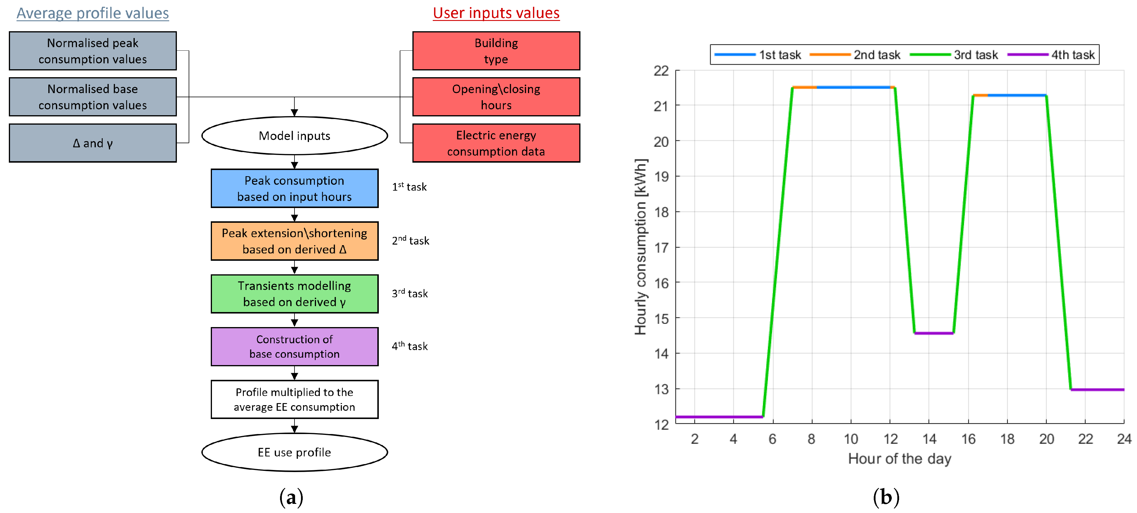
2.2. Integration of the EE Use Profile in RECON Beta Testing Environment

The EE use profiles obtained in Section 2.1 were modeled by knowing a priori the hourly EE consumption of the OLSR and their opening and closing times; the RECON software (V2.2.1), on the other hand, has, as inputs, only the opening and closing times, the type of building (minimarket or superstore), and an aggregate energy consumption value, be it monthly or annual divided into the three time slots defined by the National Energy Authority ARERA [65]. Hence, the model that is developed to generate the EE use profiles of retail buildings is based solely on these three inputs.
During the analysis aimed at modeling the EE use profile (Section 2.1), it emerged that it is defined by four variables:
-
The normalized values of peak consumption;
-
The normalized values of base consumption, i.e., associated with the closing periods;
-
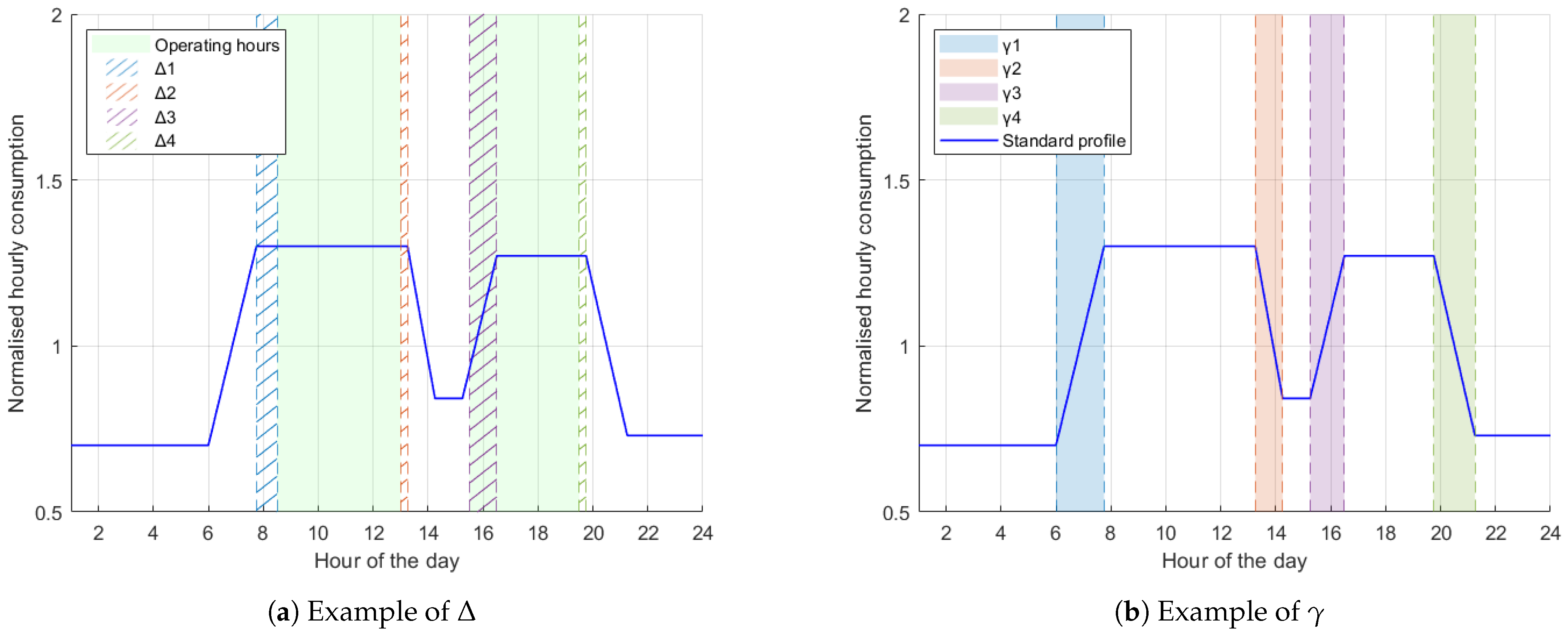
The difference between the OLSR’s actual opening/closing hours and the opening/closing hours derived from the reference database in Section 2.1, defined as Δ (one value for each opening/closing);
-
The duration of the transition periods between base load and peak load (hereinafter also called “transients” for brevity), defined as γ (one value for each transient).
It is important to note that the parameters Δ and γ do not find direct correspondence in the existing literature; however, they emerged as particularly insightful during our data analysis. For this reason, it was decided to integrate them into the model on the basis of the empirical insights obtained during data analysis. Two examples of Δ and γ are depicted in Figure 2a,b.
The retail buildings, and hence, their consumption profiles, were divided into two categories, minimarkets and superstores, to reflect their differing operational characteristics. The peak and base values of the profiles were determined by calculating the median of the normalized peaks and bases from the EE use profile for each category. Although the normalized peak consumption values are comparable between the two retail types, they were treated separately to generate specific consumption profiles: the minimarket consumption profiles are generated using the minimarket peak values, and the superstore consumption profiles using the superstore peak values. Minimarkets, which experience an intra-day break, have two distinct peak consumption values and three base consumption values; in contrast, the superstores exhibit one peak consumption value and two base consumption values. These values were then saved into a vector format, one for the superstore (S, Equation (9)) and one for the minimarket (M, Equation (10)). The former is defined by three values: one value for the peak (defined as P O ) and two values for the two different bases (defined as b O 1 and b O 2 ). The latter is composed of five values: two values for the two different peaks (defined as P I 1 and P I 2 ) and three values for the three different bases (defined as b I 1 , b I 2 and b I 3 ).
The obtained vectors are reported in Equations (9) and (10):
S = b O 1 P O b O 2
M = b I 1 P I 1 b I 2 P I 2 b I 3
The first and third element of the S vector represent the base values of the profile, while the second defines the peak value.
Differently, the second and fourth element of the M vector represent the peak values, while the first, third, and fifth element define the base values.
Then, the difference ( Δ ) between the actual opening hours and the opening hours defined on the basis of the database are estimated for each month of the year.
The monthly values were used for the generation of the monthly EE use profile, while, for the yearly profile, the mode for Δ i is considered, as the mean and median returned decimal values that were not easily convertible into an hourly format.
Lastly, the study of transients is performed. In this instance, the OLSRs were divided into two categories: superstore and minimarket.
The γ values are then evaluated on a monthly basis and, similarly to the Δ values, the monthly values were used for the generation of the monthly EE use profile, while, for the yearly profile, the mode for γ i is considered.
The implemented model use the following logic (also represented in Figure 3):
  • The duration of peak consumption is modeled using the input hours, and then, the model extends or reduces the duration of peak consumption based on the reference Δ ;
  • Then, it constructs the transients by considering their duration ( γ ), after which it fills the base segments of the remaining sections;
  • Finally, the model calculates the average hourly consumption using the aggregated EE data and multiplies the modeled normalized profile with the value just obtained, in order to have an estimated hourly consumption profile on a daily basis.
Therefore, the numerical model is able to construct a reference energy consumption profile that best fits the OLSR being simulated, given only the opening and closing times and an aggregated monthly or annual energy consumption value.

2.3. Validation of the Model

To validate the model, its outputs profiles were compared with real profiles from data of an Italian building, which were not a part of the dataset used in Section 2.1, as well as with data from three American commercial buildings, selected from the OEDI database [66], located in the same climatic zone of Milan, from which the reference profiles in Section 2.1 were generated. This validation was carried out by computing the relative deviation between the model-generated consumption profile and the real profiles, as given by Equation (6).
The used data for the validation underwent the same filtering and cleaning process described earlier in Section 2.1. Then, the model was provided with the three essential inputs required to generate the consumption profile (the same inputs required by the RECON software): an aggregate energy consumption value (monthly or yearly), the type of building, and the operating hours of the OLSR. Finally, the consumption profile generated was compared with the real one.
Since the model developed allows the use of two types of consumption values, annual and monthly, the validation was carried out using both categories of data to assess the model performance.

3. Results

In this section, the results obtained using the previous methodology are presented, along with some relevant considerations.
First, the results related to the generation of the EE use profile (Section 3.1) are reported. Subsequently, the integration of the profile within RECON beta testing environment is discussed (Section 3.2), followed by the validation of the model (Section 3.3).

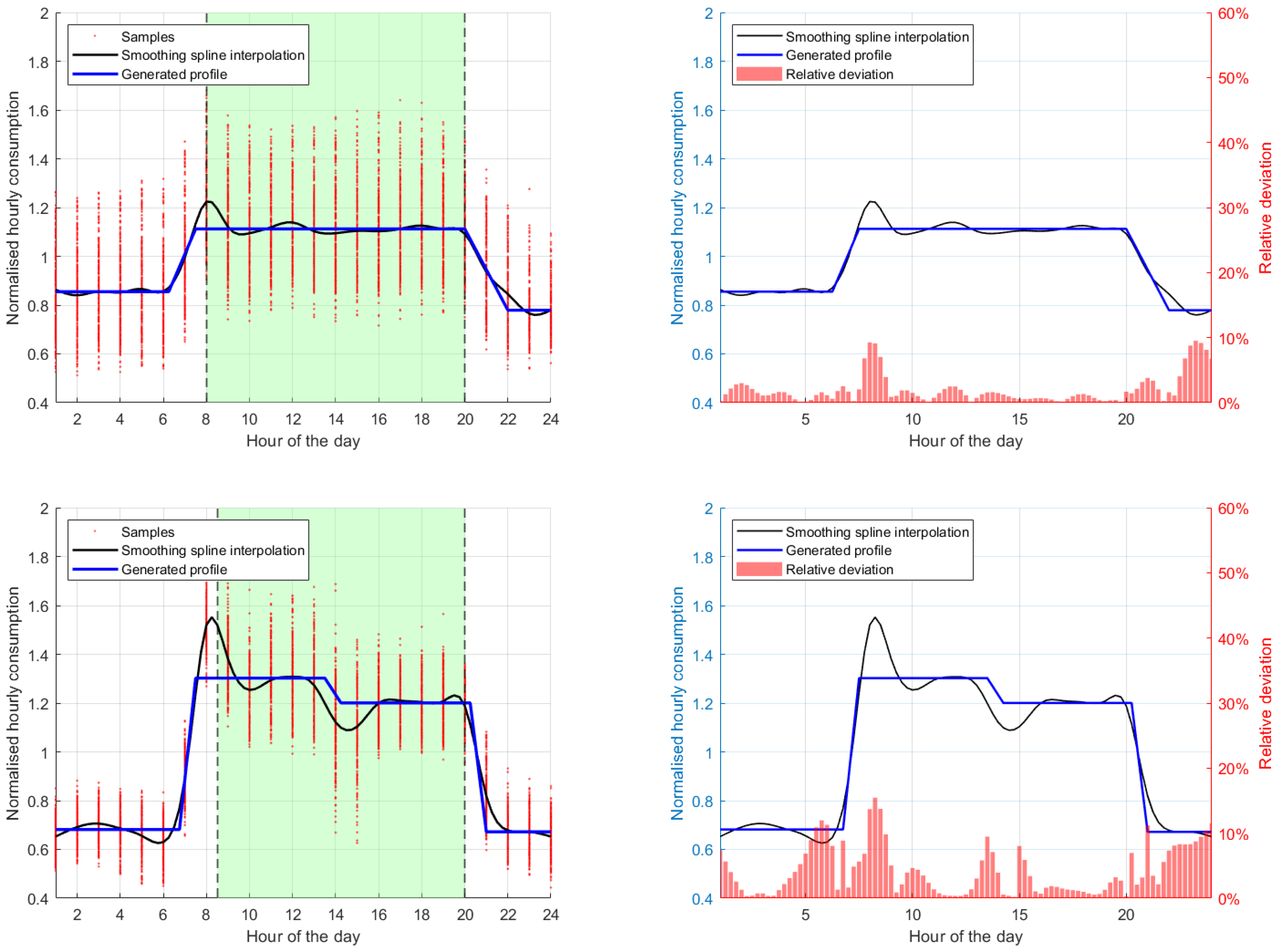
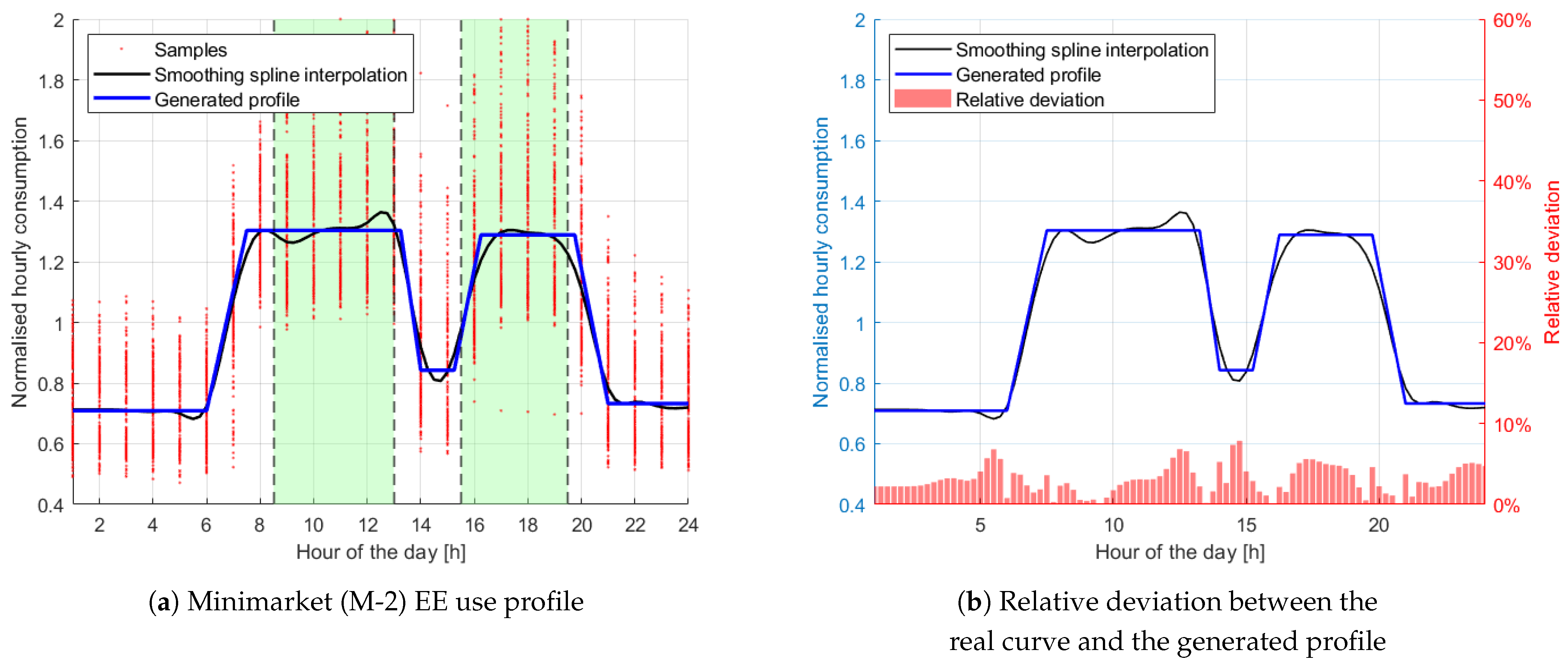
3.1. EE Use Profile Generation from Exiting Database

Before starting to generate the consumption profile, the dataset reported in Table 1 must be cleaned, which involves removing inaccurate or irrelevant records from the dataset. Moreover, days corresponding to the Italian national holiday have not been considered. Figure 4a,b shows the datasets before and after the cleaning process.
Starting from the selected data, the EE use profile can be generated on a yearly basis. Following the steps outlined in Section 2.1, an EE use profile for each available OLSR is modeled. Each profile represents the normalized average hourly electric energy consumption in a day. Figure 5a shows the generated profile while Figure 5b shows the trend of the relative deviation (Equation (6)).
In Figure 5a the blue curve is the generated profile, the light green background indicates the OLSR’s opening hours, the black curves is the smoothing spline interpolation, the red dots represent the data in the n E day , i vectors, and the red bars, in Figure 5b, represent the relative deviation (see Equation (6)) between the profile generated in blue and the interpolating curve in black. The resulting profile has an average relative deviation around 3.10%.
Only one profile obtained through the developed model is presented in this section; additional results can be found in Appendix A. Table 3 lists the obtained results for the other OLSRs analyzed.

3.2. Integration of the EE Use Profile into RECON Beta Testing Environment

This section focuses on the methodology to integrate the model in RECON beta testing environment. RECON requires an input only the opening/closing time of the OLSR, the type of building, and an aggregate EE consumption value, be it monthly or annual.
During the analysis carried out in Section 2.1, it emerged that the EE use profile is defined by four variables. These four variables are then derived in order to implement the model.
The peak and base values were determined by calculating the median of the peaks and bases of the reference energy consumption profiles for the available OLSRs, divided in superstores and minimarkets. These values were then saved into a vector, one for the superstore (S) and one for the minimarket (M), which are defined by the values:
S = 0.72 1.22 0.72
M = 0.73 1.31 0.84 1.34 0.76
The first and third elements of the S vector represent the base values of the profile, while the second defines the peak value. Differently, the second and fourth elements of the M vector represent the peak values, while the first, third, and fifth elements define the base values.
Then, the difference between the OLSR’s actual opening hours and the opening hours defined by the model ( Δ ) are estimated. These differences are defined for each month, as reported in Table 4.
A negative value of Δ means that the profile generated by the model anticipate the OLSR’s actual opening/closing hours, while a positive value of Δ means that the profile generated by the model is delayed with respect to the OLSR’s actual opening/closing hours. For example, Δ = −1 means that the generated peak profile will start one hour before of the actual opening/closing time, whereas Δ = 0.75 means that the generated peak profile will start 45 min after the actual opening/closing time.
These values were used for the modeling of the monthly reference energy consumption profile, while, for the yearly profile, the mode for each column is considered.
Lastly, the study of transients is performed. In this instance, the OLSRs were divided into the two categories. Results are reported in Table 5.
These values were used for the modeling of the monthly reference energy consumption profile, while, for the yearly profile, the mode for each column is considered.
The model, given only the opening and closing times and an aggregated monthly or annual energy consumption value, can generate a consumption profile that fits the OLSR being simulated. This profile is built using the four variables previously defined.

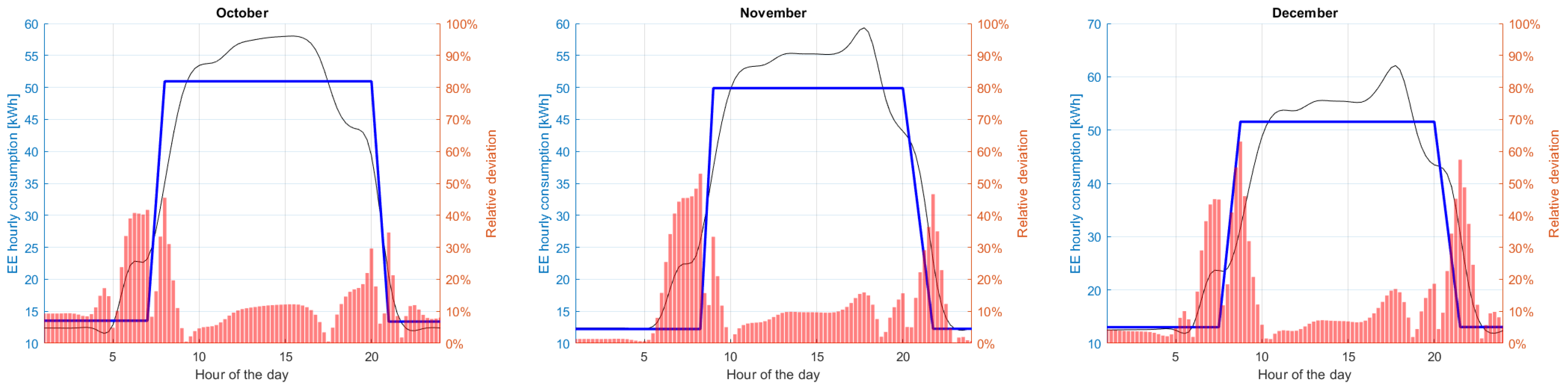
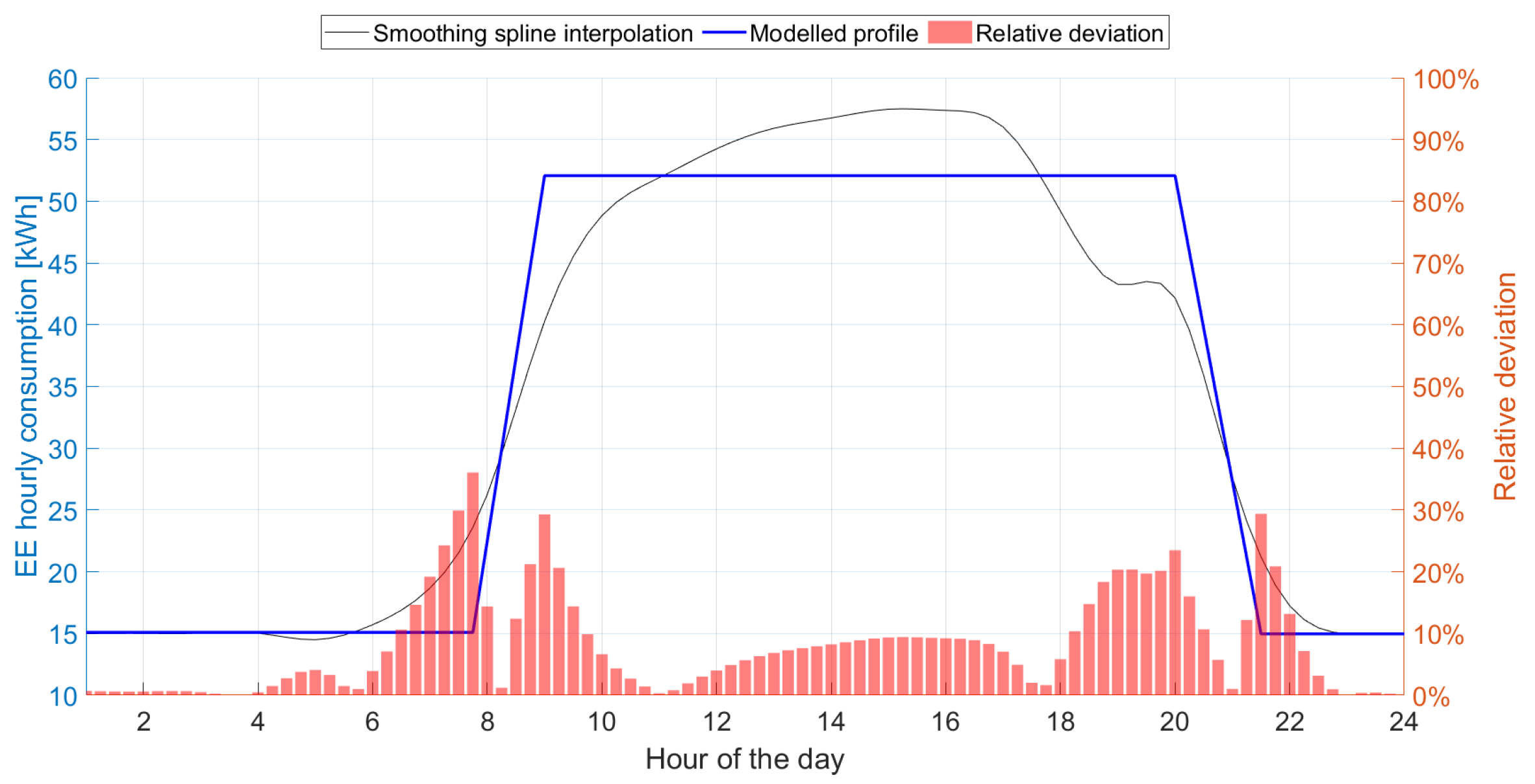
3.3. Validation of the Model

To validate the developed model, consumption data from OEDI dataset [66] have been used, alongside data from an additional OLSR that have not been used for the model development. To select the data most consistent with the data of the OLSRs used for developing the model, it was necessary to identify a city included in the OEDI dataset that falls within the same climate zone as the analyzed facilities. The city selected is Baltimore, in the state of Maryland, which falls in the Cfa zone in the Köppen classification [47] or in the 4A zone following the ANSI/ASHRAE Standard 169-2020 [67] (the same as Milan). Three different buildings configuration were considered for this study, but only one is reported in this chapter; the other can be found in Appendix B.
The model was first validated using data from a OLSR located nearby the OLSRs that provided the data for its development. The OLSR used for the validation is characterized by the data reported in Table 1.
The data were filtered and cleaned as previously described in Section 2.1. After completing these steps, the three essential inputs required to model the profile (i.e., the same inputs required by the RECON software) were provided to the code: an aggregated energy consumption value (either monthly or annual), the type of building (minimarket for this analysis) and the OLSR’s opening and closing hours.
The first validation was conducted on an annual basis by providing the model with the OLSR opening and closing hours and a single aggregated energy consumption value, specifically, the OLSR annual energy consumption. This value was obtained using Equation (1) and it was equal to 19.2 kWh. The result is shown in Figure 6.
Figure 6 shows the hourly consumption in the average day of the year obtained by real EE data; the model-generated profile is shown in blue and the relative deviations are represented by the bars.
As noticeable from the bar graph, the generated profile does not deviate significantly from the actual profile, with an average relative deviation of 4.93%. The largest discrepancies occur during the opening and closing transients, the latter having the greatest impact.
For the validation based on monthly data, the model was provided with the same three inputs: the opening and closing hours and a 1x12 EE consumption vector. The results can be seen in Figure 7.
As previously described, the actual consumption curve is shown in black, the generated profile in blue, and the relative deviation in red, represented by the bar chart.
Unlike the annual-based profile, it can be observed that the relative deviation between the actual and generated profile reaches values up to 40% during the periods from January to March and from November to December, which correspond to the months when heating systems are in operation. During the summer period (June–August) the average deviation lowers, with a value of about 12%.
The model was subsequently tested using the same procedure as above, on data from the OEDI dataset; the case study used for the simulation is called Strip Mall [68] and it is the one that, due to its configuration, is most similar to the analyzed OLSRs. Since no information about this structure are available, it is not possible to conduct further analyses regarding the discrepancies between the actual and generated profiles. The annual simulation, using 300.5 MWh as the yearly electric consumption, gives the results in Figure 8.
The result obtained on an annual basis is, nonetheless, acceptable, with an average relative deviation of 8.21%. However, the main issues regard the transients. The simulation is then repeated on a monthly basis. The obtained results are shown in Figure 9.
The profile generated by the model on a monthly basis is not as accurate as the annual-based one, with errors reaching peaks of 55–60% during some transients. However, given the lack of information about the structure, it can still be noted that the model performs reasonably well, taking into account that it is aimed at preliminary and feasibility energy analysis.
The validation demonstrated that the implemented model can replicate hourly EE use profiles of retail buildings with acceptable relative deviations on a yearly basis. Higher discrepancies found with hourly profiles of the average monthly day in the winter season suggest that further developments of the model should focus on the effects of heating systems on EE consumption of retail buildings.

4. Discussion

Analyzing the results of the developed algorithm, which are presented in Section 3.1 and Appendix A, it can be seen that the model is able to generate a fairly reliable electric energy use profile from the raw data. However, the algorithm struggles to model certain transient dynamics when the deviation between data points is small, which leads to an inaccurate representation of the profile (see the final profile in Figure A1). In the future, an improvement could be to enhance the resolution of the algorithm so that it can capture even minor deviations in the data.
Before turning to the analysis of the results of the model, it is important to emphasize that the implemented model is fundamentally data-driven. While more complex models, particularly those based on machine learning, were considered, they proved unsuitable for this study since the available dataset comprises only seven buildings, which would not provide a sufficient basis for the training required by those techniques. Consequently, employing these methods could have resulted in lower accuracy and higher computational costs, due to the limited datasets.
Turning to the analysis of the annual results, these demonstrate that the model has a good ability to reproduce the daily electricity consumption profiles, although small discrepancies can be observed, particularly during the mid-day transients. A possible future development will be to update the model so that it can handle better both opening and closing times during the day, thereby improving the transition periods.
From the monthly results (see Figure 7) in addition to the deviation mentioned above, there is a difference in the peak consumption between the modeled and the actual profiles. This discrepancy, which is more pronounced in the winter months, could be due to the operation of heat pumps, which increase electrical consumption. In future work, the model could be further developed to take into account the different types of heating systems, thereby adjusting the construction of the electricity consumption profile accordingly.
Although the model was validated and obtained good results, the validation was limited to OLSRs that are similar to the one used for the model development. Furthermore, since the validation was performed using data from Northern Italy, the results obtained may be less accurate if the model is applied to an OLSR in different locations.
For this reason, it would be desirable in the future to validate the developed model using data from other Italian regions to obtain a model that is as accurate as possible. This would be a valuable enhancement, as it could subsequently be integrated into RECON, enabling it to simulate more realistic scenarios. In addition, the model’s robustness could be further improved by training and validating it on a larger dataset. Finally, another potential application of the model could be its use for simulating consumption profiles different from those of large-scale retail, such as office buildings, and evaluate its accuracy.
It is also important to note that the development of this model has been undertaken with particular reference to the requirements of the REC, thereby ensuring that its design and implementation are fully aligned with the needs of Renewable Energy Community initiatives. Moreover, for the purpose of incentive calculations, the daily hourly profiles are scaled by the actual number of operating days of the store, while for closure days, a flat profile equal to the store’s base consumption is assumed. It is worth noting that an additional refinement could involve the introduction of typical profiles for closure days. However, such days are rare in this category, given that superstores and minimarkets are generally open seven days a week.

5. Conclusions

The presented study deals with the implementation of a data-driven model that generates, in an automatic way, electric energy use profiles for organized large-scale retail to be used in RECON beta testing. The methodology involved pre-processing and normalizing raw hourly consumption data from OLSRs, followed by the generation of representative energy use profiles. These profiles are used as a reference for the model development, which is then validated using different data from the one used for the model development. The data used for the model development come from real buildings.
From the presented work, the following conclusions are drawn:
  • The developed algorithm successfully generates normalized EE use profiles for both minimarkets and superstores starting from raw data;
  • A data-driven model was successfully developed and integrated in the RECON beta testing environment, allowing electric energy use profile generation with minimal inputs (opening/closing times, building type, and aggregated consumption);
  • Validation on an annual basis demonstrated a low mean average relative deviation (approximately 4–11%), while monthly simulations highlighted larger discrepancies during cold months, likely due to heating system influences;
  • These results indicate that while the model is robust for overall consumption trends, further refinement is needed to accurately capture transient behaviors and climatic factors.
These findings open up future developments in enhancing model accuracy, such as expanding the database of case studies for training purposes, incorporating additional variables (such as specific heating system characteristics), validating the model across different geographical regions, and extending the methodology to a wider range of commercial building types. Moreover, if in the future a large database becomes available, machine learning techniques could be implemented to reduce computational costs.

Author Contributions

Conceptualization, M.C. and F.C.; methodology, S.L, M.C., and F.C.; software, S.L. and D.F.; validation, S.L. and D.F.; formal analysis, D.F.; resources, M.C.; data curation, S.L.; writing—original draft preparation, S.L.; writing—review and editing, S.L., M.C., M.F., D.F., and F.C.; supervision, M.C., M.F., and F.C.; project administration, M.C. and F.C.; funding acquisition, M.C. All authors have read and agreed to the published version of the manuscript.

Funding

This research was funded by the “Electrical System Research” Programme Agreement 2022-2024 between ENEA and the Italian Ministry of the Environment and Energy Security, funding number (CUP) I53C22003070001.

Data Availability Statement

The data are not publicly available due to privacy restrictions.

Acknowledgments

A special thanks to Stefano Scala and Maria Adele Prosperoni of Confcooperative for their assistance, and to all the people of Confcooperative Lombardia and Milano e dei Navigli who have provided the real data used for the model calibration and validation.

Conflicts of Interest

The authors declare no conflicts of interest.

Abbreviations

The following abbreviations are used in this manuscript:
ANNArtificial Neural Network
ARERAAutorità di Regolazione per Energia Reti e Ambiente
CNNConvolutional Neural Networks
EEElectric Energy
EUEuropean Union
EVElectric Vehicle
OLSROrganized Large-Scale Retail
RECRenewable Energy Community
RECONRenewable Energy Community ecONomic simulator
REDRenewable Energy Directive
RESRenewable Energy Source
SMESmall and Medium Enterprise
SVRSupport Vector Regression

Appendix A

This appendix serves to showcase the electric energy use profiles modeled through the algorithm defined in Section 2.1. All the profiles, except for the one presented in Section 3.1, modeled by the developed algorithm for each available retail building, are presented. Figure A1 shows the OLSR profiles derived and used for the development of the model implemented in the RECON beta testing environment.
Figure A1. Profile modeled compared to the real data (on the left) and the relative deviation (on the right).
Energies 18 02368 g0a1aEnergies 18 02368 g0a1b

Appendix B

This appendix serves to showcase the validation on the other two dataset coming from the OEDI database [66]. The first analysis presented was conducted on the building called Supermarket [69] on an annual basis, with a relative deviation equal to 9.69%. The result is shown in Figure A2.
Figure A2. Daily EE use profile modeled on a yearly basis, OEDI data [66].
Energies 18 02368 g0a2
The monthly validations are shown in Figure A3.
Figure A3. Monthly profile model validation, OEDI data [66].
Energies 18 02368 g0a3
The analysis presented next was conducted on a building called Stand-alone Retail [70] on an annual basis, with a relative deviation equal to 12.61%. The result is shown in Figure A4.
Figure A4. Daily EE use profile modeled on a yearly basis, OEDI data [66].
Energies 18 02368 g0a4
The monthly validations are shown in Figure A5.
Figure A5. Monthly profile model validation, OEDI data [66].
Energies 18 02368 g0a5aEnergies 18 02368 g0a5b
Notably, the relative deviation between the modeled and real profiles is higher compared to the other analyzed cases. This discrepancy may be attributed to several factors. For instance, the exact opening and closing times of the analyzed retail buildings were not available, and assumptions had to be made in order to utilize the implemented model. Additionally, differences in electrical consumption between American and European buildings, as well as variations in the design of the heating and air conditioning systems, which were not precisely specified, could have contributed to the observed deviations. For these reasons, it is challenging to definitively pinpoint the cause of the higher relative deviation between the model-generated profile and the real profile.

References

  1. European Commission. 2050 Long-Term Strategy. Available online: https://climate.ec.europa.eu/eu-action/climate-strategies-targets/2050-long-term-strategy_en (accessed on 2 February 2025).
  2. European Commission. The European Green Deal. 11 December 2019. Available online: https://eur-lex.europa.eu/resource.html?uri=cellar:b828d165-1c22-11ea-8c1f-01aa75ed71a1.0002.02/DOC_1&format=PDF (accessed on 2 February 2025).
  3. Ahmad, T.; Zhang, D. A critical review of comparative global historical energy consumption and future demand: The story told so far. Energy Rep. 2020, 6, 1973–1991. [Google Scholar] [CrossRef]
  4. Mehedintu, A.; Sterpu, M.; Soava, G. Estimation and Forecasts for the Share of Renewable Energy Consumption in Final Energy Consumption by 2020 in the European Union. Sustainability 2018, 10, 1515. [Google Scholar] [CrossRef]
  5. European Commission. Directive (EU) 2018/2001 of the European Parliament and of the Council on the Promotion of the Use of Energy from Renewable Sources. 11 December 2018. Available online: https://eur-lex.europa.eu/legal-content/IT/TXT/PDF/?uri=CELEX:32018L2001 (accessed on 7 February 2025).
  6. European Commission. Directive (EU) 2023/2413 of the European Parliament and of the Council of 18 October 2023 Amending Directive (EU) 2018/2001, Regulation (EU) 2018/1999 and Directive 98/70/EC as Regards the Promotion of Energy from Renewable Sources, and Repealing Council Directive (EU) 2015/652. 18 October 2023. Available online: https://eur-lex.europa.eu/legal-content/EN/TXT/PDF/?uri=OJ:L_202302413 (accessed on 7 February 2025).
  7. Rossetto, N. Beyond Individual Active Customers: Citizen and Renewable Energy Communities in the European Union. IEEE Power Energy Mag. 2023, 21, 36–44. [Google Scholar] [CrossRef]
  8. Soeiro, S.; Ferreira Dias, M. Renewable energy community and the European energy market: Main motivations. Heliyon 2020, 6, e04511. [Google Scholar] [CrossRef]
  9. Ahmed, S.; Ali, A.; D’Angola, A. A Review of Renewable Energy Communities: Concepts, Scope, Progress, Challenges, and Recommendations. Sustainability 2024, 16, 1749. [Google Scholar] [CrossRef]
  10. Bauwens, T. Explaining the diversity of motivations behind community renewable energy. Energy Policy 2016, 93, 278–290. [Google Scholar] [CrossRef]
  11. Hanke, F.; Lowitzsch, J. Empowering Vulnerable Consumers to Join Renewable Energy Communities—Towards an Inclusive Design of the Clean Energy Package. Energies 2020, 13, 1615. [Google Scholar] [CrossRef]
  12. Soeiro, S.; Ferreira Dias, M. Community renewable energy: Benefits and drivers. Energy Rep. 2020, 6, 134–140. [Google Scholar] [CrossRef]
  13. Veronese, E.; Lauton, L.; Barchi, G.; Prada, A.; Trovato, V. Impact of Non-Residential Users on the Energy Performance of Renewable Energy Communities Considering Clusterization of Consumptions. Energies 2024, 17, 3984. [Google Scholar] [CrossRef]
  14. Tatti, A.; Ferroni, S.; Ferrando, M.; Motta, M.; Causone, F. The Emerging Trends of Renewable Energy Communities’ Development in Italy. Sustainability 2023, 15, 6792. [Google Scholar] [CrossRef]
  15. ENEA. RECON—Simulatore per Comunità Energetiche Rinnovabili. 2024. Available online: https://recon.smartenergycommunity.enea.it/ (accessed on 13 March 2025).
  16. Gestore dei Servizi Energetici (GSE). Portale Autoconsumo—Comunità Energetiche Rinnovabili. 2024. Available online: https://www.autoconsumo.gse.it/ (accessed on 13 March 2025).
  17. E-360. E-360—Soluzioni per Comunità Energetiche. 2024. Available online: https://www.e-360.it/ (accessed on 13 March 2025).
  18. MyGreenEnergy. Costruisci la tua Comunità Energetica—Simulatore. 2024. Available online: https://www.mygreenenergy.it/costruisci-la-tua-comunita-energetica#calcola (accessed on 13 March 2025).
  19. Giannuzzo, L.; Minuto, F.D.; Schiera, D.S.; Lanzini, A. Reconstructing hourly residential electrical load profiles for Renewable Energy Communities using non-intrusive machine learning techniques. Energy AI 2024, 15, 100329. [Google Scholar] [CrossRef]
  20. Di Silvestre, M.L.; Montana, F.; Sanseverino, E.R.; Sciumè, G.; Zizzo, G. An algorithm for renewable energy communities designing by maximizing shared energy. In Proceedings of the 2023 AEIT International Annual Conference (AEIT), Rome, Italy, 5–7 October 2023; pp. 1–6. [Google Scholar]
  21. Di Somma, M.; Dolatabadi, M.; Burgio, A.; Siano, P.; Cimmino, D.; Bianco, N. Optimizing virtual energy sharing in renewable energy communities of residential users for incentives maximization. Sustain. Energy Grids Netw. 2024, 39, 101492. [Google Scholar] [CrossRef]
  22. Belloni, E.; Fioriti, D.; Poli, D. Optimal design of renewable energy communities (RECs) in Italy: Influence of composition, market signals, buildings, location, and incentives. Electr. Power Syst. Res. 2024, 235, 110895. [Google Scholar] [CrossRef]
  23. Sun, Y.; Haghighat, F.; Fung, B.C. A review of the-state-of-the-art in data-driven approaches for building energy prediction. Energy Build. 2020, 221, 110022. [Google Scholar] [CrossRef]
  24. Amasyali, K.; El-Gohary, N.M. A review of data-driven building energy consumption prediction studies. Renew. Sustain. Energy Rev. 2018, 81, 1192–1205. [Google Scholar] [CrossRef]
  25. Pan, Y.; Zhang, L. Data-driven estimation of building energy consumption with multi-source heterogeneous data. Appl. Energy 2020, 268, 114965. [Google Scholar] [CrossRef]
  26. Liu, H.; Liang, J.; Liu, Y.; Wu, H. A Review of Data-Driven Building Energy Prediction. Buildings 2023, 13, 532. [Google Scholar] [CrossRef]
  27. Wei, Y.; Zhang, X.; Shi, Y.; Xia, L.; Pan, S.; Wu, J.; Han, M.; Zhao, X. A review of data-driven approaches for prediction and classification of building energy consumption. Renew. Sustain. Energy Rev. 2018, 82, 1027–1047. [Google Scholar] [CrossRef]
  28. Ferrando, M.; Banfi, A.; Causone, F. Changes in energy use profiles derived from electricity smart meter readings of residential buildings in Milan before, during and after the COVID-19 main lockdown. Sustain. Cities Soc. 2023, 99, 104876. [Google Scholar] [CrossRef]
  29. Huang, Y.; Xiong, N.; Liu, C. Renewable energy technology innovation and ESG greenwashing: Evidence from supervised machine learning methods using patent text. J. Environ. Manag. 2024, 370, 122833. [Google Scholar] [CrossRef]
  30. Lari, A.J.; Sanfilippo, A.P.; Bachour, D.; Perez-Astudillo, D. Using Machine Learning Algorithms to Forecast Solar Energy Power Output. Electronics 2025, 14, 866. [Google Scholar] [CrossRef]
  31. Mikkola, J.; Lund, P.D. Models for generating place and time dependent urban energy demand profiles. Appl. Energy 2014, 130, 256–264. [Google Scholar] [CrossRef]
  32. Wang, Z.; Hong, T. Generating realistic building electrical load profiles through the Generative Adversarial Network (GAN). Energy Build. 2020, 224, 110299. [Google Scholar] [CrossRef]
  33. Lombardi, F.; Balderrama, S.; Quoilin, S.; Colombo, E. Generating high-resolution multi-energy load profiles for remote areas with an open-source stochastic model. Energy 2019, 177, 433–444. [Google Scholar] [CrossRef]
  34. Bayram, I.S.; Saffouri, F.; Koc, M. Generation, analysis, and applications of high resolution electricity load profiles in Qatar. J. Clean. Prod. 2018, 183, 527–543. [Google Scholar] [CrossRef]
  35. Rana, M.; Sethuvenkatraman, S.; Goldsworthy, M. A data-driven approach based on quantile regression forest to forecast cooling load for commercial buildings. Sustain. Cities Soc. 2022, 76, 103511. [Google Scholar] [CrossRef]
  36. Granell, R.; Axon, C.J.; Kolokotroni, M.; Wallom, D.C. A reduced-dimension feature extraction method to represent retail store electricity profiles. Energy Build. 2022, 276, 112508. [Google Scholar] [CrossRef]
  37. Orr, M. Short-Term Electrical Load Forecasting for Irish Supermarkets with Weather Forecast Data. Ph.D. Thesis, National College of Ireland, Dublin, Ireland, 2021. [Google Scholar]
  38. Chuan, L.; Ukil, A. Modeling and Validation of Electrical Load Profiling in Residential Buildings in Singapore. IEEE Trans. Power Syst. 2015, 30, 2800–2809. [Google Scholar] [CrossRef]
  39. Czétány, L.; Vámos, V.; Horváth, M.; Szalay, Z.; Mota-Babiloni, A.; Deme-Bélafi, Z.; Csoknyai, T. Development of electricity consumption profiles of residential buildings based on smart meter data clustering. Energy Build. 2021, 252, 111376. [Google Scholar] [CrossRef]
  40. Khan, A.N.; Iqbal, N.; Rizwan, A.; Ahmad, R.; Kim, D.H. An Ensemble Energy Consumption Forecasting Model Based on Spatial-Temporal Clustering Analysis in Residential Buildings. Energies 2021, 14, 3020. [Google Scholar] [CrossRef]
  41. Ramírez-Mendiola, J.L.; Grünewald, P.; Eyre, N. The diversity of residential electricity demand – A comparative analysis of metered and simulated data. Energy Build. 2017, 151, 121–131. [Google Scholar] [CrossRef]
  42. Khan, I.; Jack, M.W.; Stephenson, J. Identifying residential daily electricity-use profiles through time-segmented regression analysis. Energy Build. 2019, 194, 232–246. [Google Scholar] [CrossRef]
  43. Batra, N.; Parson, O.; Berges, M.; Singh, A.; Rogers, A. A comparison of non-intrusive load monitoring methods for commercial and residential buildings. arXiv 2014, arXiv:1408.6595. [Google Scholar] [CrossRef]
  44. Coakley, D.; Raftery, P.; Keane, M. A review of methods to match building energy simulation models to measured data. Renew. Sustain. Energy Rev. 2014, 37, 123–141. [Google Scholar] [CrossRef]
  45. MathWorks. Matlab R2024b. 2024. Available online: https://it.mathworks.com/products/new_products/latest_features.html (accessed on 27 March 2025).
  46. European Commission. Directive 2004/22/EC of the European Parliament and of the Council of 31 March 2004 on Measuring Instruments. Available online: https://eur-lex.europa.eu/legal-content/EN/TXT/PDF/?uri=CELEX:32014L0032 (accessed on 22 February 2025).
  47. Köppen, W. Klassification der Klimate nach Temperatur, Niederschlag und Jahreslauf. 1918. Available online: https://koeppen-geiger.vu-wien.ac.at/pdf/Koppen_1918.pdf (accessed on 17 February 2025).
  48. Huang, G. Missing data filling method based on linear interpolation and lightgbm. J. Phys. Conf. Ser. 2021, 1754, 012187. [Google Scholar] [CrossRef]
  49. Mohamed Noor, N.; Yahaya, A.S.; Ramli, N.; Abdullah, M.M.A.B. Filling Missing Data Using Interpolation Methods: Study on the Effect of Fitting Distribution. Key Eng. Mater. 2013, 594–595, 889–895. [Google Scholar] [CrossRef]
  50. Murti, D.M.P.; Pujianto, U.; Wibawa, A.P.; Akbar, M.I. K-Nearest Neighbor (K-NN) based Missing Data Imputation. In Proceedings of the 2019 5th International Conference on Science in Information Technology (ICSITech), Yogyakarta, Indonesia, 23–24 October 2019; pp. 83–88. [Google Scholar] [CrossRef]
  51. Batista, G.E.; Monard, M.C. A study of K-nearest neighbour as an imputation method. In Proceedings of the Soft Computing Systems—Design, Management and Applications, HIS 2002, Santiago, Chile, 1–4 December 2002; Volume 87, p. 48. [Google Scholar]
  52. Ma, X.; Han, Y.; Qin, H.; Wang, P. KNN data filling algorithm for incomplete interval-valued fuzzy soft sets. Int. J. Comput. Intell. Syst. 2023, 16, 30. [Google Scholar] [CrossRef]
  53. Zhang, S. Nearest neighbor selection for iteratively kNN imputation. J. Syst. Softw. 2012, 85, 2541–2552. [Google Scholar] [CrossRef]
  54. Ishwaran, H.; Kogalur, U.B.; Blackstone, E.H.; Lauer, M.S. Random survival forests. Ann. Appl. Stat. 2008, 2, 841–860. [Google Scholar] [CrossRef]
  55. Xia, J.; Zhang, S.; Cai, G.; Li, L.; Pan, Q.; Yan, J.; Ning, G. Adjusted weight voting algorithm for random forests in handling missing values. Pattern Recognit. 2017, 69, 52–60. [Google Scholar] [CrossRef]
  56. Tang, F.; Ishwaran, H. Random forest missing data algorithms. Stat. Anal. Data Min. Asa Data Sci. J. 2017, 10, 363–377. [Google Scholar] [CrossRef] [PubMed]
  57. Humaira, H.; Rasyidah, R. Determining The Appropiate Cluster Number Using Elbow Method for K-Means Algorithm. In Proceedings of the 2nd Workshop on Multidisciplinary and Applications (WMA), Padang, Indonesia, 24–25 January 2020. [Google Scholar] [CrossRef]
  58. Syakur, M.A.; Khotimah, B.K.; Rochman, E.M.S.; Satoto, B.D. Integration K-Means Clustering Method and Elbow Method for Identification of The Best Customer Profile Cluster. IOP Conf. Ser. Mater. Sci. Eng. 2018, 336, 012017. [Google Scholar] [CrossRef]
  59. Cui, M. Introduction to the K-Means Clustering Algorithm Based on the Elbow Method. Geosci. Remote Sens. 2020, 3, 9–16. [Google Scholar] [CrossRef]
  60. Cerquitelli, T.; Chicco, G.; Corso, E.D.; Ventura, F.; Montesano, G.; Armiento, M.; González, A.M.; Santiago, A.V. Clustering-Based Assessment of Residential Consumers from Hourly-Metered Data. In Proceedings of the 2018 International Conference on Smart Energy Systems and Technologies (SEST), Seville, Spain, 10–12 September 2018; pp. 1–6. [Google Scholar] [CrossRef]
  61. Berggren, B.; Wall, M. Two Methods for Normalisation of Measured Energy Performance—Testing of a Net-Zero Energy Building in Sweden. Buildings 2017, 7, 86. [Google Scholar] [CrossRef]
  62. Wendland, H.; Rieger, C. Approximate Interpolation with Applications to Selecting Smoothing Parameters. Numer. Math. 2005, 101, 729–748. [Google Scholar] [CrossRef]
  63. Haszpra, L.; Prácser, E. Uncertainty of hourly-average concentration values derived from non-continuous measurements. Atmos. Meas. Tech. 2021, 14, 3561–3571. [Google Scholar] [CrossRef]
  64. The MathWorks, I. Fminbnd. 2006. Available online: https://it.mathworks.com/help/releases/R2024b/matlab/ref/fminbnd.html (accessed on 29 March 2025).
  65. ARERA. Fasce Orarie. Available online: https://www.arera.it/bolletta/glossario-dei-termini/dettaglio/fasce-orarie (accessed on 29 March 2025).
  66. N.R.E. Laboratory, Commercial Reference Buildings. 2014. Available online: https://en.openei.org/datasets/files/961/pub/ (accessed on 21 December 2024).
  67. ASHRAE Climatic Data for Building Design Standards. 2021. Available online: https://www.ashrae.org/file%20library/technical%20resources/standards%20and%20guidelines/standards%20addenda/169_2020_a_20211029.pdf (accessed on 15 October 2024).
  68. Deru, M.; Field, K.; Studer, D.; Benne, K.; Griffith, B.; Torcellini, P.; Liu, B.; Halverson, M.; Winiarski, D.; Rosenberg, M.; et al. Commercial Reference Building: Strip Mall. 2014. Available online: https://data.openei.org/submissions/169 (accessed on 3 October 2024).
  69. Deru, M.; Field, K.; Studer, D.; Benne, K.; Griffith, B.; Torcellini, P.; Liu, B.; Halverson, M.; Winiarski, D.; Rosenberg, M.; et al. Commercial Reference Building: Supermarket. 2014. Available online: https://data.openei.org/submissions/170 (accessed on 3 October 2024).
  70. Deru, M.; Field, K.; Studer, D.; Benne, K.; Griffith, B.; Torcellini, P.; Liu, B.; Halverson, M.; Winiarski, D.; Rosenberg, M.; et al. Commercial Reference Building: Stand-Alone Retail. 2014. Available online: https://data.openei.org/submissions/168 (accessed on 3 October 2024).
Figure 1. Data pre-processing steps.
Energies 18 02368 g001
Figure 2. Visual representation of (a) Δ and (b) γ .
Energies 18 02368 g002
Figure 3. (a) Flowchart of the implemented model. (b) Visual representation of the developed model.
Energies 18 02368 g003
Figure 4. Comparison between (a) raw and (b) cleaned datasets for Minimarket (M-4).
Energies 18 02368 g004
Figure 5. Comparison between (a) electricity use profile and (b) relative deviation from the generated profile for Minimarket (M-2).
Energies 18 02368 g005
Figure 6. Minimarket M-1 (Table 1) yearly profile model validation.
Energies 18 02368 g006
Figure 7. Minimarket M-1 (Table 1) monthly profile model validation. In each subplot, the black line represents the reference (smoothing spline interpolation), the blue line shows the modeled profile, and the red bars indicate the relative deviation.
Energies 18 02368 g007
Figure 8. Daily reference consumption profile modeled on a yearly basis, OEDI data [66].
Energies 18 02368 g008
Figure 9. Monthly profile model validation, OEDI data [66].
Energies 18 02368 g009aEnergies 18 02368 g009b
Table 1. Analyzed OLSRs.
ReferenceTypeTotal Area
[m2]
Power at
the Net
Meter [kW]
Installed
PV Capacity
[kW]
EV
Charging
Station
M-1Minimarket 113015-No
M-2Minimarket113063-No
M-3Minimarket1309100-No
M-4Minimarket45075-No
S-1Superstore2247250-No
S-2Superstore2730250-No
S-3Superstore956949863.75Yes
1 Used for the validation of the model.
Table 2. Useful data for generating profile consumption.
VariablesUnit of Measure
Location-
Opening hours-
Hourly electric consumption [ kWh ]
Total area [ m 2 ]
Grid meter active power [ kW ]
Nominal installed PV power [ kW ]
Nominal installed Electric vehicles (EV) charging station power [ kW ]
Table 3. Obtained results for the EE use profile.
ReferenceTypeAverage Relative Deviation [%]
M-1Minimarket 1-
M-2Minimarket3.10
M-3Minimarket2.82
M-4Minimarket3.29
S-1Superstore2.05
S-2Superstore4.30
S-3Superstore3.99
1 Used for the validation of the model.
Table 4. Monthly values for Δ 1, Δ 2, Δ 3, and Δ 4.
Month Δ 1 Δ 2 Δ 3 Δ 4
January−10.250.750
February−10.250.750
March−100.750
April−1−0.250.750
May−10.250.750.25
June00.250.750
July0.250.250.50
August0.2500.750
September−10.250.750
October−100.750
November−10.250.750
December−1.2500.750
Mode−10.250.750
Table 5. Monthly values of γ 1, γ 2, γ 3, and γ 4. (a) Minimarket values. (b) Superstore values.
Month γ 1 γ 2 γ 3 γ 4
January1.5111.25
February1111.25
March1.25111.5
April1.5111.75
May1.25111.75
June1.50.7511.75
July1.5111.75
August1.511.251.75
September1.5111.25
October1.51.2511.25
November1.50.7511.25
December1.511.251.5
Mode1.5111.25
(a)
Month γ 1 γ 2 γ 3 γ 4
January1.25--1.25
February1.25--1.25
March1.25--1.25
April1--1.5
May1--1.5
June1.5--1.5
July1.75--1.5
August1.25--1.5
September1--1.5
October1--1
November0.75--1.75
December1.25--1.5
Mode1.25--1.5
(b)
Disclaimer/Publisher’s Note: The statements, opinions and data contained in all publications are solely those of the individual author(s) and contributor(s) and not of MDPI and/or the editor(s). MDPI and/or the editor(s) disclaim responsibility for any injury to people or property resulting from any ideas, methods, instructions or products referred to in the content.

