A Fault Diagnosis Framework for Pressurized Water Reactor Nuclear Power Plants Based on an Improved Deep Subdomain Adaptation Network

Abstract

Fault diagnosis in pressurized water reactor nuclear power plants faces the challenges of limited labeled data and severe class imbalance, particularly under Design Basis Accident (DBA) conditions. To address these issues, this study proposes a novel framework integrating three key stages: (1) feature selection via a signed directed graph to identify key parameters within datasets; (2) temporal feature encoding using Gramian Angular Difference Field (GADF) imaging; and (3) an improved Deep Subdomain Adaptation Network (DSAN) using weighted Focal Loss and confidence-based pseudo-label calibration. The improved DSAN uses the Hadamard product to achieve feature fusion of ResNet-50 outputs from multiple GADF images, and then aligns both global and class-wise subdomains. Experimental results show that, on the transfer task from the NPPAD source set to the PcTran-simulated AP-1000 target set across five DBA scenarios, the framework raises the overall accuracy from 72.5% to 80.5%, increases macro-F1 to 0.75 and AUC-ROC to 0.84, and improves average minority-class recall to 74.5%, outperforming the original DSAN and four baselines by explicitly prioritizing minority-class samples and mitigating pseudo-label noise. However, our evaluation is confined to simulated data, and validating the framework on actual plant operational logs will be addressed in future work.

1. Introduction

The stable operation of nuclear power plants (NPPs) is crucial for energy security, carbon emission reduction, economic benefits, and nuclear safety. Fault diagnosis, which involves analyzing operational data to detect and address potential anomalies in time, is a key technology for ensuring the safe operation of NPPs. Current fault diagnosis approaches can be broadly classified into knowledge-driven and data-driven methods [1]. Knowledge-driven approaches rely on expert experience and physical models, yet their applicability is often constrained in complex systems. In contrast, data-driven methods leverage deep learning to automatically extract features, making them well-suited for handling complex nonlinear problems and demonstrating significant potential.

A wide range of intelligent fault diagnosis methods based on data-driven approaches have been explored for NPPs. For instance, Min et al. (2019) developed a pattern recognition method based on Auto-Associative Kernel Regression (AAKR) [2]; Li et al. (2020) proposed an unsupervised transient identification model using clustering methods and Convolutional Neural Networks (CNNs) [3]; Yue et al. (2023) introduced a signal reconstruction method for steam generator (SG) water levels based on a Deep Residual Shrinkage Network (DRSN) [4]; and Tonday Rodriguez et al. (2024) proposed a hierarchical deep learning framework combining multi-class and one-class classifiers [5].

Despite their success, data-driven fault diagnosis methods still face significant challenges. First, the high cost of data annotation in NPPs results in limited labeled datasets, leading to the small-sample problem [6]. Second, operational data from NPPs significantly outweigh fault data, causing a severe class imbalance issue [7]. These limitations hinder the effective application of conventional deep learning approaches.

To address the challenges of small sample sizes and data imbalance, various solutions have been proposed. For example, Yin et al. (2024) introduced a deep learning-based fault diagnosis method utilizing Adaptive Synthetic Sampling (ADASYN) to augment imbalanced samples [8]; Li et al. (2024) proposed a human-in-the-loop self-improving small-sample fault diagnosis approach [9]; and Dai et al. (2023) developed an intelligent fault diagnosis method based on a Generative Adversarial Network (GAN), specifically the GRU-BEGAN framework [10].

These methods have demonstrated effectiveness in specific scenarios under the assumption that the training and testing data come from the same operational conditions. However, the operational conditions of nuclear power plants vary according to demand in practical situations, such as adjusting power levels to accommodate fluctuations in the power grid. In this case, the distribution discrepancy between the training and testing data is inevitable, which may affect the model’s diagnostic performance. Additionally, requiring the training data to cover all operational conditions to improve model performance is unrealistic, as collecting and labeling sufficient samples is a labor-intensive and time-consuming task [11].

Therefore, transfer learning, which aims to transfer knowledge from the source domain to the target domain to address issues such as data distribution discrepancies and the scarcity of labeled data, may offer a more advantageous solution when handling data with significant differences from various nuclear power plants [12]. Various subspace mapping techniques, such as Transfer Component Analysis (TCA) and Joint Distribution Adaptation (JDA) [13,14], have been proposed to reduce domain discrepancies by projecting data into a shared low-dimensional subspace for cross-domain feature alignment. Ganin et al. (2017) introduced the Domain-Adversarial Neural Network (DANN),which employs adversarial training to learn domain-invariant representations [15]. Zhu et al. (2017) combined GANs with transfer learning in CycleGAN to enable unsupervised image-to-image translation [16].

However, existing models primarily focus on reducing global distribution shifts between the source and target domains without ensuring intra-domain feature alignment. This may lead to inconsistencies in feature distributions within the domain, impairing the model’s ability to capture fine-grained local features and significantly degrading performance in fine-grained classification tasks. Zhu et al. (2020) proposed the Deep Subdomain Adaptation Network (DSAN) [17], which not only aligns global distributions between the source and target domains but also enhances intra-domain feature alignment by dividing the domain into multiple subdomains and aligning corresponding subdomains. Consequently, the DSAN offers unique advantages in transfer learning. Nonetheless, the DSAN has limitations under extreme small-sample and class-imbalanced conditions: it tends to overfit in severely data-scarce scenarios due to insufficient symmetric alignment; furthermore, it lacks dedicated optimization for minority-class samples in the target domain, leading to suboptimal classification performance under class imbalance.

Although deep learning models offer high accuracy in fault diagnosis for nuclear power plants, their internal decision-making processes remain opaque—the so-called “black box” problem—which severely limits their practical application in a safety-critical, transparency-demanding industry like nuclear power [18]. Operators must clearly understand the logic behind model predictions to make rapid, effective decisions. Purely data-driven approaches often overlook the intrinsic physical causal relationships in nuclear systems, so their explanations may not align with actual plant behavior, making interpretability essential. Recent studies have begun to quantify feature contributions using methods such as SHAP to enhance diagnostic transparency [19]. Moreover, integrating domain priors or alternative techniques is crucial: for example, embedding physical-mechanism models such as signed directed graphs or Bayesian networks into the architecture, or constructing physics–data fusion models [20,21,22]. Such multi-source strategies not only improve transparency but also bolster model robustness and generalization, providing more reliable technical support for nuclear safety operations.

To address these limitations, this paper proposes an improved DSAN-based fault diagnosis framework for pressurized water reactor nuclear power plants. First, based on the fault propagation pathways of NPPs, we select and retain 19 key parameters that significantly influence system behavior, applying dimensionality reduction to both source and target domain data [23]. The reduced-dimensional data are then partitioned into multiple one-dimensional vector groups and transformed into Gramian Angular Field (GAF) images after normalization [24]. Finally, a weighted Focal Loss function is introduced to the DSAN to enhance sensitivity to minority-class samples, while incorporating a confidence-based pseudo-label calibration mechanism to improve fault classification under small-sample and class-imbalanced conditions.

The key contributions of this work include the following:

(1)

proposing an improved DSAN-based fault diagnosis framework;

(2)

introducing weighted Focal Loss to enhance classification performance for minority-class samples, as well as incorporating a confidence-based pseudo-label calibration mechanism to improve fault classification in small-sample and class-imbalanced scenarios.

This paper is organized as follows: Section 1 provides an introduction, Section 2 describes the proposed framework, Section 3 presents experimental analyses, and Section 4 concludes the study.

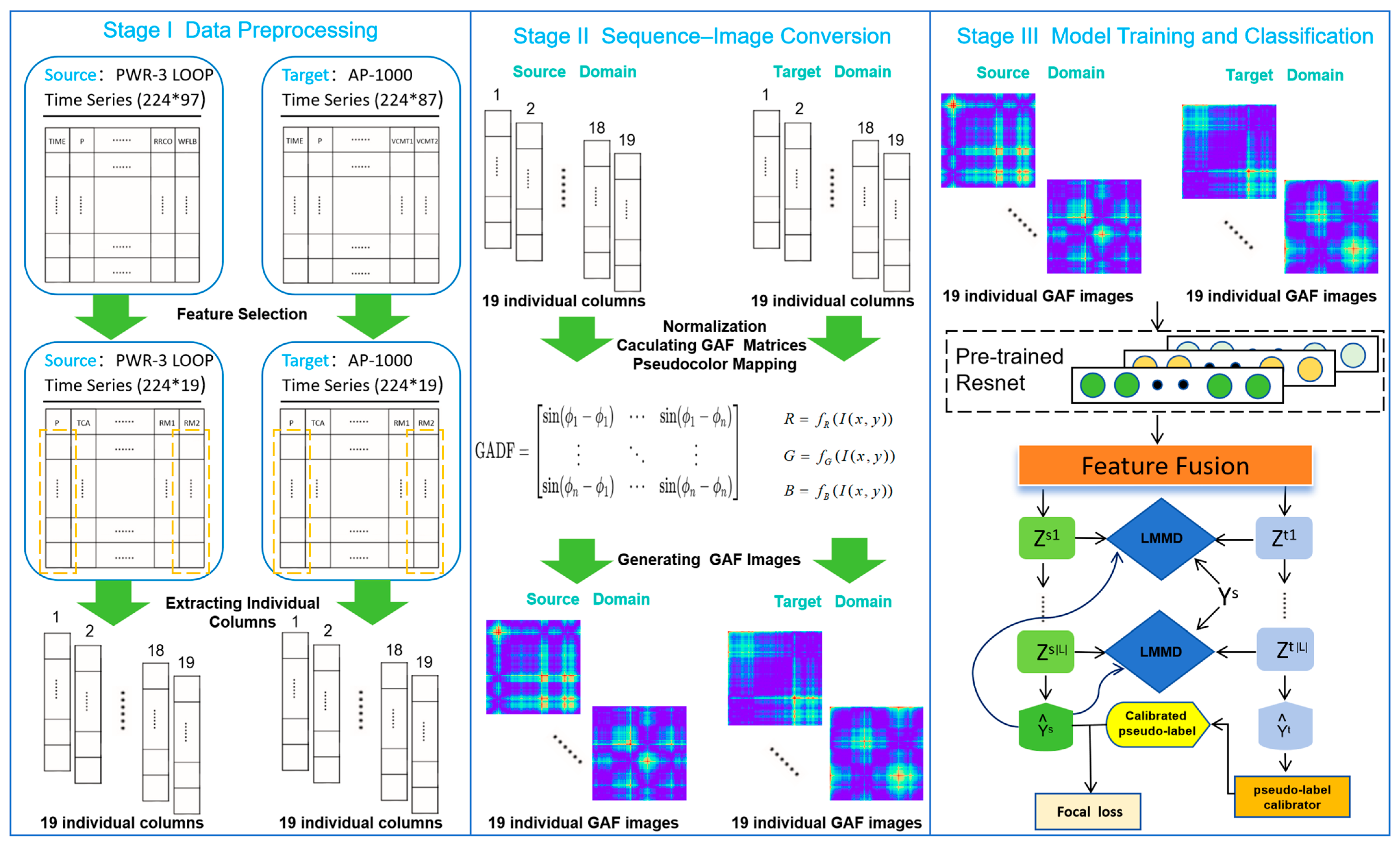
2. Fault Diagnosis Framework Based on an Improved DSAN

To address the challenges of small sample sizes and class imbalance in nuclear power plant fault diagnosis, this paper proposes a fault diagnosis framework based on an improved DSAN. As shown in Figure 1, the framework consists of three parts:

• Stage I—Data Preprocessing:

Key physical parameters highly correlated with DBAs are selected using a signed directed graph. The raw data are then filtered and segmented into one-dimensional vectors to reduce redundancy and computational complexity.

• Stage II—Sequence–Image Conversion:

The preprocessed time-series data are normalized and later converted into GAF images, which effectively preserve temporal characteristics while mitigating interference among parameters.

• Stage III—Model Training and Classification:

The GAF images obtained from both the source and target domains are used as inputs for training and classification using the improved DSAN. This stage enhances the classification performance on minority-class samples under conditions of small sample sizes and class imbalance, while also improving fine-grained feature alignment between subdomains.

2.1. Data Preprocessing

2.1.1. Datasets

This paper uses an open-source dataset, Nuclear Power Plant Accident Data (NPPAD), provided by Qi et al. (2022), as source domain data for model pre-training [25]. This open-source dataset was constructed using the nuclear power plant simulation software PcTran (https://github.com/thu-inet/NuclearPowerPlantAccidentData, 30 March 2025) to simulate a PWR 3 Loop nuclear power plant, generating data under different operational conditions. The dataset consists of several 2D parameter matrices. In the source domain dataset, each sample contains 97 parameters. Additionally, to simulate the small sample sizes and class-imbalance conditions present in nuclear power plant fault diagnosis, the paper uses data from a PcTran (version 1.0.1) simulation of an AP-1000 nuclear power plant under various operating conditions as target domain data. Each sample in the target domain dataset contains 87 parameters. Both the source and target domain datasets include data from five different operating conditions under full power, with varying fault sizes. This study selects operating conditions involving MSLB, LOCA, and SGTR (A) and SGTR (B), as well as normal conditions (see

Table 1. Operating conditions selected in the simulation experiment.

ID	Labels	Operation Conditions	Severity (Sample Number Per Category)
			Source Domain	Target Domain
0	NORMAL	Normal operation	Null (200)	Null (200)
1	LOCA	Loss of coolant accident in hot leg	1~100% (100)	2, 4, …, 100 (50)
2	MSLB	Main steam line break outside containment	1~100% (100)	2, 4, …, 100 (50)
3	SGTR (A)	Steam generator A tube rupture	1~100% (100)	2, 4, …, 100 (50)
4	SGTR (B)	Steam generator B tube rupture	1~100% (100)	2, 4, …, 100 (50)

).

For data collection, both the source and target domain datasets use a unified nuclear plant runtime of 2240 s, with fault introduction occurring at the 10th second. The data collection interval is 10 s, resulting in 224 rows of data for both the source and target domains. The labels, severities, and sample counts of the operating conditions in the source and target domain datasets are shown in Table 1. In the source domain dataset, there are 200 normal operation samples and 100 samples for each of the other four fault conditions. In the target domain dataset, there are 100 normal operation samples and 50 samples for each of the other four fault conditions, simulating the small sample sizes and class-imbalance conditions in nuclear power plant fault diagnosis. Specifically, the ratio of normal operation samples to all other fault conditions is 1:1.

2.1.2. Feature Selection

Nuclear power plant operating data are characterized by high dimensionality, redundancy, and noise. The high-dimensional data generated by numerous sensors contain many correlated variables, but not all are equally important for fault diagnosis [26]. Additionally, measurement noise and outliers in the data may interfere with the model’s diagnostic capability, while the scarcity of DBAs and sample imbalance further complicate the diagnosis [27]. Furthermore, real-time fault diagnosis is required in nuclear power plants, and processing high-dimensional data significantly increases computational complexity, hindering rapid response.

In nuclear power plant fault diagnosis, feature selection techniques can extract key fault-related parameters from a large amount of sensor data, reducing the demand for computational resources while preventing overfitting or performance degradation caused by unnecessary features, thus improving diagnostic accuracy and interpretability [28]. Therefore, feature selection not only enhances model performance but also maintains an intuitive understanding of the system’s operational mechanisms, thereby better assisting in the analysis of fault causes.

An effective strategy in feature selection is to incorporate prior knowledge from nuclear power plants. SDG is a causal-based modeling approach primarily used to describe the logical relationships between system variables [29]. It consists of nodes (representing variables or fault sources) and signed directed edges (representing causal relationships), where the sign indicates the positive or negative influence between variables. The fault propagation pathway is a specific application of SDG in fault diagnosis, which reveals how a fault propagates through the system by influencing other system variables via causal relationships [30]. By combining the SDG fault propagation pathway with feature selection, it is possible to identify the key parameters that are closely related to fault occurrences, thereby improving both the accuracy and interpretability of the fault diagnosis. This approach not only effectively leverages existing domain knowledge but also enhances model performance while increasing the reliability of diagnostic results.

Liu et al. (2018) [31] introduced an SDG-based approach in the field of nuclear power plant fault diagnosis and successfully constructed an SDG model for fault propagation analysis in PWRs. The model defines key parameter nodes and causal relationships related to faults, establishing the fault propagation pathway for the primary loop cooling system in a nuclear plant. This pathway graph visually represents how faults propagate through the system, covering all possible paths from the fault source to affected nodes through forward and backward reasoning, ensuring comprehensive fault diagnosis. This method facilitates the rapid identification of root causes and potential impacts, with causal chain reasoning providing clear physical explanations for diagnostic results. It is well-suited for fault diagnosis in small-sample and high-dimensional systems.

This paper’s feature selection process is based on the SDG model developed by Liu et al. (2018) [31], where parameters highly correlated with DBAs are selected for dimensionality reduction, as shown in Figure 2. The parameter definitions in the fault propagation pathway (SDG model) are provided in

Table 2. Key parameters for nuclear power plant fault diagnosis.

ID	Node Label	Node Name	ID	Node Label	Node Name
1	P	Pressure of RCS	11	WRCB	Coolant flow of loop B
2	TCA	Temperature of cold leg A	12	WSTA	Steam flow of SG A
3	TCB	Temperature of cold leg B	13	WSTB	Steam flow of SG B
4	QMWT	Total thermal power	14	TRB	Temperature reactor building
5	QMGA	Power of SG A heat removal	15	PRB	Pressure reactor building
6	QMGB	Power of SG B heat removal	16	RM1	Rad monitor reactor building air
7	WFWA	Feed-water flow of SG A	17	RM2	Rad monitor steam line
8	WFWB	Feed-water flow of SG B	18	NSGA	Level SG A narrow range
9	VOL	Volume of RCS liquid	19	NSGB	Level SG B narrow range
10	WRCA	Coolant flow of loop A

,while the definitions of the operation conditions are listed in Table 1.

Following these processes, the source and target domain datasets are standardized to 224 rows and 19 columns. The data in each column are then normalized.

2.1.3. Extracting Individual Columns

In multidimensional data, different parameters have distinct physical meanings, dimensions, or statistical properties, and these differences can lead to the weakening or masking of certain parameters’ features during overall analysis. By extracting individual columns from the data, the independent characteristics of each parameter can be better preserved, ensuring that the contribution of each parameter in subsequent processing is fully reflected. Moreover, this method effectively reduces errors introduced by correlations or cross-interference between parameters, thereby improving the accuracy of data analysis. Therefore, this paper extracts individual columns from the 224 rows and 19 columns of the dimensionality-reduced data samples, retaining the original features of the data and minimizing mutual interference between parameters.

2.2. Sequence–Image Conversion

2.2.1. Gramian Angular Field

GAF is a technique for converting one-dimensional time-series signals into two-dimensional images, widely used in deep learning for time-series data analysis. It maps time-series data into a polar coordinate system and utilizes the mathematical properties of the Gramian matrix to represent the temporal dependencies, periodicity, and correlations of the time series in an image format.

GAF preserves the original time series’ characteristics while amplifying relevant patterns, enabling deep learning models to extract features more effectively. There are two forms of GAF: Gramian Angular Summation Field (GASF) and Gramian Angular Difference Field (GADF) [24]. Since GADF focuses more on local variations and can capture short-term fluctuations and anomalies, making it beneficial for anomaly detection, this paper adopts GADF.

The transformation process of GADF first requires normalizing the time series. The normalization formula for time-series data is defined as follows in Equation (1):

$${\tilde{x}}_i=2{\displaystyle \frac{x_i-\min (X)}{\max (X)-\min (X)}}-1$$

(1)

where ${\tilde{x}}_i$ is the normalized value of the i-th data point in the time series, while max(X) and min(X) represent the maximum and minimum values of the time series, respectively. Equation (1) normalizes the original time series $X=\{x_1,x_2,\dots ,x_n\}$ to the range [−1, 1] to meet the requirements of polar coordinate mapping. Normalization eliminates differences in data scales, ensuring a uniform range. In deep learning tasks, normalization can also accelerate training convergence and improve model performance. The calculation of angle ${\varphi }_i$ is shown in Equation (2):

$${\varphi }_i=\arccos ({\tilde{x}}_i)$$

(2)

According to Equation (2), the normalized time-series data ${\tilde{x}}_i$ are mapped to the i-th angle ${\varphi }_i$. In the polar coordinate system, the numerical characteristics of time points are represented by angles. This transformation preserves the temporal dependencies of the time series, making the representation of time-series features more intuitive in the angular space. The calculation of GADF is shown in Equation (3):

$${\mathrm{GADF}}_{i,j}=\sin ({\varphi }_i-{\varphi }_j)$$

(3)

where $\sin ({\varphi }_i-{\varphi }_j)$ represents the product of the differences between points i and j. Equation (3) emphasizes the differences between time points (rather than their positive correlation) by computing the sine values of the angular differences between each pair of time points. This approach is well-suited for capturing dynamic changes and non-periodic features.

2.2.2. Pseudo-Color Mapping

The GADF matrix obtained through the above Gramian Angular Field transformation can be used to generate a single-channel grayscale image. Pseudo-color mapping is a technique that converts single-channel grayscale images into color images [32]. Its core idea is to use a color mapping function to map grayscale values into a color space (such as the RGB space), thereby enhancing the visual effect of the image or highlighting certain features. This paper employs a mapping function for each color channel as shown in Equation (4), where linear interpolation is used to transform grayscale values into the corresponding RGB channels:

$$\mathrm{R}=f_R(I(x,y)),\hspace{1em}\mathrm{G}=f_G(I(x,y)),\hspace{1em}\mathrm{B}=f_B(I(x,y))$$

(4)

In this formula, R, G, and B represent the red, green, and blue channels of the image, respectively. The functions $f_R$, $f_G$, and $f_B$ are designed to map the grayscale values to the RGB channels. Specifically, low grayscale values are mapped to blue, intermediate values are mapped to green, and high grayscale values are mapped to red. This color mapping enhances the visual effect of the image by emphasizing different levels of intensity in the data.

2.3. Model Training and Classification

2.3.1. Pre-Trained Resnet

In this study, the ResNet-50 feature extractor embedded in the DSAN is initialized with ImageNet-pre-trained weights. Yosinski et al. [33] demonstrated that low-level convolutional kernels transfer well across domains, whereas high-level semantics lose transferability as the domain gap widens. To prevent such natural-image priors from dominating the representation of GAF maps, which encode temporal correlations rather than object semantics, we freeze all convolutional and BatchNorm parameters and replace the original classifier with a newly initialized head consisting of a global average pooling layer, a fully connected layer mapping 2048 to 512 units, a ReLU activation layer, a dropout layer (rate = 0.5), and a final fully connected layer mapping 512 to C classes. GAF inputs are resized to 224 × 224, normalized with the ImageNet mean and variance, and augmented by ±10° rotations, horizontal/vertical flips, and Gaussian noise (σ ≤ 0.01). The head is optimized with AdamW (lr = 1 × 10⁻³, weight_decay = 1 × 10⁻⁴) under a StepLR schedule (decay factor = 0.1 every 30 epochs); training runs for 50 epochs with early stopping (patience = 10) and five-fold cross-validation. Fine-tuning samples are drawn from NPPAD scenarios disjoint from the test conditions to avoid data leakage and enhance generalization. Comparable “frozen-backbone, head-only” strategies have proved effective in time-series-to-image classification: Wang and Oates [34] encoded UCR sequences as GAF/MTF images and lifted the mean accuracy from 71% to 83% with a head-only tiled CNN; Hatami et al. [35] attained 93% mean accuracy on 20 UCR datasets by fine-tuning only upper CNN layers on recurrence plots; and Lu et al. [36] froze a ResNet-50 backbone for GAF-based bearing-fault diagnosis and gained a 2.2-pp improvement over full fine-tuning. Collectively, these studies substantiate the scientific validity of the fully frozen-backbone protocol adopted here.

2.3.2. Feature Fusion

In deep learning models, feature fusion is the process of effectively combining features from multiple different sources to obtain more enriched information. In this study, we employ the Hadamard product and summation for feature fusion. Specifically, the feature fusion step involves the following key operations:

• Initialization of weights

To ensure weight diversity and prevent issues such as gradient vanishing or exploding during the early stages of training, the weight matrix $W_1,W_2,\dots ,W_{19}$ is randomly initialized according to a standard normal distribution, as shown in Equation (5):

$$W_i\sim N(0,1),i=1,2,\dots ,19$$

(5)

This initialization method provides a good starting point for the network, helping to accelerate convergence and avoid premature local optima.

2.

Hadamard product and feature weighting

For the features extracted from each image, we perform the Hadamard product operation to element-wise multiply the features with their corresponding weights, thereby applying weighting to the features extracted from each image. For the features extracted from the i-th image, this is represented by Equation (6):

$$X_{i^{\prime }}=W_i\circ X_i,\hspace{1em}i=1,2,\dots ,19$$

(6)

where $\circ$ denotes the Hadamard product [37], $W_i$ is the weight vector corresponding to the features extracted from the i-th image, and $X_i$ represents the features extracted from the i-th image. Through the Hadamard product, the features extracted from each image are weighted to reflect their importance in the overall input.

3.

Feature summation

All the weighted features are summed to obtain a consolidated feature representation, resulting in a fused feature that represents the entire time series, as shown in Equation (7):

$$X_{\mathrm{final}}={\displaystyle \sum _{i=1}^{19}{X}_{i^{\prime }}}.$$

(7)

4.

Non-linear activation

To enhance the expressive capacity of the network, the summed features $X_{\mathrm{final}}$ are processed through a non-linear activation function tanh [38], as shown in Equation (8). The activation function helps the model capture more complex non-linear relationships and restricts the feature values within the range of [−1, 1], thereby improving the stability and robustness of the model.

$$\tanh (x)={\displaystyle \frac{e^x-e^{-x}}{e^x+e^{-x}}}$$

(8)

5.

Backpropagation and weight update

The final features $X_{\mathrm{final}}$ obtained through feature fusion are processed through a non-linear activation function and then used as the model’s input. After passing through subsequent layers, the output is compared with the true labels to compute the loss function $L$. During the backpropagation process, the gradient of the loss function is propagated back to the weight matrix using the chain rule to update the weights. Specifically, the gradient update rule is shown in Equation (9):

$$W_i=W_i-\eta \cdot {\displaystyle \frac{\partial L}{\partial W_i}},$$

(9)

where $\eta$ is the learning rate, and ${\displaystyle \frac{\partial L}{\partial W_i}}$ is the gradient of the loss function with respect to the weights. Through backpropagation, the model can adjust the weights, thereby improving its ability to learn the weighted features.

2.3.3. DSAN

Local Maximum Mean Discrepancy (LMMD) is one of the key improvements of the DSAN. LMMD is an extension of the traditional Maximum Mean Discrepancy (MMD), specifically designed for subdomain feature alignment with class information. Compared to the standard MMD, which focuses solely on matching overall distributions, LMMD further considers the distributional differences between different classes, thereby improving cross-domain adaptability. In the DSAN, subdomains are divided by class, with each class corresponding to a subdomain. Therefore, the calculation of LMMD is shown in Equation (10):

$${\widehat{d}}_{\mathcal{H}}(p,q)={\displaystyle \frac{1}{C}}{\displaystyle \sum _{c=1}^C{‖{\displaystyle \sum _{x_i^s\in D_s}{w}_i^{sc}}\varphi (x_i^s)-{\displaystyle \sum _{x_j^t\in D_t}{w}_j^{tc}}\varphi (x_j^t)‖}_{\mathcal{H}}^2}$$

(10)

where C is the number of classes, with each class C corresponding to a subdomain; and $\varphi (x)$ is the feature mapping function that maps input samples to a high-dimensional Reproducing Kernel Hilbert Space (RKHS). After activation with different Gaussian kernels, LMMD achieves subdomain alignment in different dimensions. $w_i^c$ is the sample weight under class C, defined as shown in Equation (11):

$$w_i^c={\displaystyle \frac{y_{ic}}{{\displaystyle \sum _{(x_j,y_j)\in D}{y}_{jc}}}}$$

(11)

The weights $w_i^c$ are used to balance the contributions of each class, ensuring that each class plays its corresponding role in the feature alignment process. Additionally, the source domain data use the true labels, while the target domain data use the probability distribution predicted by the network. The expansion of LMMD is shown in Equation (12):

$${\widehat{d}}_l(p,q)={\displaystyle \frac{1}{C}}{\displaystyle \sum _{c=1}^C\left[{\displaystyle \sum _{i=1}^{n_s}{\displaystyle \sum _{j=1}^{n_s}{w}_i^{sc}}}{w}_j^{sc}k\left(z_i^{sl},z_j^{sl}\right)+{\displaystyle \sum _{i=1}^{n_t}{\displaystyle \sum _{j=1}^{n_t}{w}_i^{tc}}}{w}_j^{tc}k\left(z_i^{tl},z_j^{tl}\right)-2{\displaystyle \sum _{i=1}^{n_s}{\displaystyle \sum _{j=1}^{n_t}{w}_i^{sc}}}{w}_j^{tc}k\left(z_i^{sl},z_j^{tl}\right)\right]}$$

(12)

The entire network is optimized using the loss function shown in Equation (13):

$${\min }_f{\displaystyle \frac{1}{n_s}}{\displaystyle \sum _{i=1}^{n_s}J}(f(x_i^s),y_i^s)+\lambda {\displaystyle \sum _{l\in L}{\widehat{d}}_l}(p,q)$$

(13)

The first term above uses cross-entropy as the classification loss, and the second term uses LMMD as the adaptive loss.

2.4. Improvements Based on DSAN

In unsupervised domain adaptation tasks, the target domain data typically lack true labels and rely on the model’s predictions to generate pseudo-labels for training. The pseudo-labels used in this paper are soft labels. However, due to cross-domain distribution bias, some pseudo-labels may contain noise, which affects the model’s convergence. Additionally, fault data from nuclear power plants often suffer from class imbalance, causing the model to be more inclined to predict the majority class, leading to a decline in classification performance for the minority class. Therefore, in the improvement of the loss function, this paper combines weighted Focal Loss (WFL) and confidence-based pseudo-label calibration (CPC), which reduces or ignores the loss impact of low-confidence samples in the target domain.

2.4.1. Confidence-Based Pseudo-Label Calibration

In the target domain, since true labels are absent, the model must generate pseudo-labels for training. However, some pseudo-labels have low confidence and may be erroneous, and using them directly could adversely affect training performance. Therefore, this paper adopts a CPC approach to adjust the contribution of pseudo-labels to the loss, such that high-confidence samples exert a greater influence while low-confidence samples have a reduced impact [39].

For target domain samples, the maximum class probability is first computed for each sample, and the class corresponding to the maximum probability is taken as the pseudo-label, as shown in Equation (14):

$${\tilde{y}}_j=\arg {\max }_k p_{j,k}$$

(14)

where $p_{j,k}$ is the probability that the sample is predicted as class k, and ${\tilde{y}}_j$ is the pseudo-label for the j-th sample. Subsequently, the paper calculates its confidence using Equation (15):

$$p_{\max }={\max }_k p_{j,k}$$

(15)

where $p_{j,k}$ denotes the probability that sample ${\mathrm{x}}_{\mathrm{j}}$ is predicted as class k; and the larger the value of $p_{\max }$, the higher the model’s confidence in classifying the sample. Conversely, if $p_{\max }$ is too low, it may indicate an erroneous pseudo-label, and its contribution to the loss should be reduced. Therefore, we introduce confidence weighting, as shown in Equation (16):

$$w_j=\max \left({\displaystyle \frac{p_{\max }-T}{1-T}},0\right)$$

(16)

where T is the confidence threshold and serves as a hyperparameter. When $p_{\max }>T$, the sample’s loss is computed in proportion to its confidence—higher confidence results in a greater contribution to the loss. When $p_{\max }\le T$, the sample is likely an erroneous pseudo-label, and its loss weight is set to 0 to reduce the impact of the incorrect pseudo-label.

The pseudo-label confidence in this paper is dynamically adjusted throughout the training process, as shown in Equation (17):

$$T(\theta )=T_0+(T_f-T_0)\cdot \theta$$

(17)

In this formulation, $T_0$ denotes the high initial confidence threshold set at the beginning of training, $T_f$ represents the lower threshold used in the later stages, and θ ∈ [0, 1] is the normalized training progress, typically computed as the ratio of the current epoch to the total number of epochs. This equation describes a linearly decreasing threshold strategy: in the early stages of training, only high-confidence pseudo-labels are accepted to ensure label reliability; and as training proceeds and the model becomes better adapted to the target domain, the threshold gradually decreases, allowing more medium-confidence samples to participate in training and expanding the coverage of pseudo-label supervision. This dynamic adjustment mechanism balances early-stage stability with late-stage data utilization, thereby enhancing the model’s generalization performance on the target domain.

2.4.2. Weighted Focal Loss

Weighed Focal Loss [40] is an improved version of cross-entropy loss designed to address the class imbalance problem. Its core ideas are as follows:

• To reduce the loss contribution of easily classified samples, thereby diminishing the dominant influence of the majority class on the loss;
• To amplify the loss contribution of hard-to-classify samples, enhancing the model’s ability to learn from minority-class samples.

To handle the class imbalance issue and the associated pseudo-label noise, this paper replaces the original cross-entropy loss with a weighted Focal Loss. This loss can assign higher weights to minority-class samples while increasing the focus on hard-to-classify samples, as shown in Equation (18):

$$F{L}_{\mathrm{weighted}}(p_t)=-w_j{\alpha }_{{\tilde{y}}_j}{(1-p_t)}^{\gamma }\log (p_t)$$

(18)

where γ controls the weight decay rate of easy-to-classify samples, adapting to small sample data. When γ = 0, the Focal Loss degenerates to the standard cross-entropy loss. A very high γ may cause the model to overly focus on minority-class samples. In this paper’s experiments, γ is set to 2 to balance class imbalance and the model’s convergence speed. ${\alpha }_{{\tilde{y}}_j}$ is the class weight. When higher weights are assigned to minority-class samples, the model will pay more attention to these samples during training, thereby improving the handling of class imbalance. ${\alpha }_{{\tilde{y}}_j}$ is used to increase the model’s learning ability for minority classes. Its computation process is shown in Equation (19).

$${\alpha }_{{\tilde{y}}_j}={\displaystyle \frac{1}{{\displaystyle \sum _{j=1}^{n_t}{w}_j}\cdot 1({\tilde{y}}_j=c)}}$$

(19)

Combined with Equation (18), the total classification loss for the target domain is calculated as shown in Equation (20):

$$L_{\mathrm{target}}=-{\displaystyle \sum _{j=1}^{n_t}{w}_j}\cdot {\alpha }_{{\tilde{y}}_j}{(1-p_{j,{\tilde{y}}_j})}^{\gamma }\log (p_{j,{\tilde{y}}_j})$$

(20)

Since there are no pseudo-labels in the source domain, the classification loss for the source domain is calculated as shown in Equation (21):

$$L_{\mathrm{source}}=-{\displaystyle \sum _{i=1}^{n_s}{\alpha }_{y_i}}{(1-p_{i,y_i})}^{\gamma }\log (p_{i,y_i})$$

(21)

The computation of Focal Loss is shown in Equation (22):

$${\mathcal{L}}_{\mathrm{focal}}={\mathcal{L}}_{\mathrm{source}}+{\mathcal{L}}_{\mathrm{target}}$$

(22)

2.4.3. Total Loss Function

The total loss function is composed of the confidence-based Focal Loss and adaptive loss for both the source domain and the target domain, as shown in Equation (23):

$$L_{\mathrm{total}}=L_{\mathrm{source}}+L_{\mathrm{target}}+\lambda L_{\mathrm{LMMD}}$$

(23)

where λ is used to trade off the domain adaptation loss and the WFL. In this study, the use of λ follows the original DSAN and is dynamically adjusted. The expansion of Equation (23) is shown in Equation (24):

$$L_{\mathrm{total}}=-{\displaystyle \sum _{i=1}^{n_s}{\alpha }_{y_i}}{(1-p_{i,y_i})}^{\gamma }\log (p_{i,y_i})-{\displaystyle \sum _{j=1}^{n_t}{w}_j}\cdot {\alpha }_{{\tilde{y}}_j}{(1-p_{j,{\tilde{y}}_j})}^{\gamma }\log (p_{j,{\tilde{y}}_j})+\lambda L_{\mathrm{LMMD}}$$

(24)

2.4.4. Mathematical Analysis

From the perspective of gradient computation, the derivative of the loss with respect to the logit $z_t$ takes the following form:

$${\displaystyle \frac{\partial {\mathcal{L}}_{\mathrm{WFL}}}{\partial z_t}}\propto w_j\cdot {\alpha }_c\cdot \gamma \cdot {(1-p_c)}^{\gamma -1}\cdot \log (p_c)\cdot (p_c-1)$$

(25)

It can be seen that the gradient magnitude is jointly regulated by the following mechanisms:

When $p_t\to 0$ (i.e., the model predicts the pseudo-label with high confidence), ${(1-p_t)}^{\gamma }\to 0$, and the gradient approaches zero, indicating that the training strength for well-learned samples is automatically suppressed;

When $p_t$ is relatively low but still greater than the threshold $T(\theta )$, WFL amplifies the corresponding loss, thereby reinforcing learning;

The class-specific weight ${\alpha }_{{\tilde{y}}_j}$ further increases the gradient magnitude for minority-class samples, effectively mitigating the training bias caused by class imbalance.

Overall, CPC controls whether a sample is selected for training (via $w_j$) to suppress label noise, while WFL determines the training weight of the selected samples (via ${\alpha }_{{\tilde{y}}_j}$ and ${(1-p_t)}^{\gamma }$). These two mechanisms work in synergy to enforce a strategy of “training only on reliable pseudo-labels and focusing on hard-to-classify samples”. This significantly enhances the model’s ability to recognize minority and ambiguous samples in the target domain, demonstrating both mathematical soundness and empirical robustness. Experimental results verify that this joint mechanism not only improves overall accuracy on the target domain but also significantly increases the recall rate of minority classes, making it a critical component of the proposed method.

3. Experiments and Analysis

3.1. Experimental Environment Configuration

The experiments in this study were conducted using PyTorch (version 2.2). The experimental environment configuration for this paper included the following: Dual Intel Xeon Gold 5215 processors, 256 GB DDR4 memory, and NVIDIA Tesla V100 GPU (32 GB) x2.

3.2. Experimental Design

To evaluate the performance of the fault diagnosis framework proposed in this paper, along with the improved DSAN model, on nuclear power plant fault diagnosis data under conditions of a small sample size and class imbalance, this paper uses the NPPAD dataset as the source domain dataset and data obtained from five different operating conditions of a nuclear power plant with an AP-1000 reactor type simulated by PcTran as the target domain data. Both the source and target domain data are first subjected to the same data preprocessing, with the time-series data converted into image processing. Additionally, to ensure that the processed inputs match the model, each model incorporated the feature fusion module mentioned in Section 2.3.2 of the paper. Based on this, we trained and classified the data using different transfer learning models, such as the DSAN, DANN, DAN [41], DeepCORAL [42], DAAN [43], and the improved DSAN model we proposed. By comparing these models, we explored their performance in the target domain across metrics such as classification accuracy, minority-class recall, and AUC-ROC, with a particular focus on the recognition ability for the minority class.

3.3. Training Strategy

In this study, the dataset is split into a training set, validation set, and test set in a 70%:15%:15% ratio. The training set consists mainly of source domain data and is used for model learning and domain adaptation. The validation set includes a mix of source and target domain data to monitor performance and assist in hyperparameter tuning. The test set contains only target domain data and is used for final evaluation.

Since there are no true labels for the target domain data during training, the DSAN uses a pseudo-labeling strategy. Pseudo-labels are generated through the model’s predictions on the target domain. During the training process, the target domain data are first passed through the trained network for prediction, producing output class probabilities. Based on these output probabilities, a pseudo-label (i.e., the model’s predicted class label) is assigned to each sample in the target domain. These pseudo-labels serve as the “assumed labels” for the target domain data to compute the classification loss. As training progresses, the model continuously adjusts its parameters, and the pseudo-labels are updated according to the model’s predictions.

In terms of hyperparameter selection, the experimental setup follows the original DSAN implementation:

Stochastic Gradient Descent (SGD) is used as the optimization algorithm, with the momentum set to 0.9. A dynamic learning rate decay strategy is applied, as shown in Equation (26):

$${\eta }_{\theta }={\displaystyle \frac{{\eta }_0}{{(1+\alpha \theta )}^{\beta }}}$$

(26)

where the initial learning rate is set to 0.01, α is 10, β is 0.75, and θ represents the training progress, which increases linearly from 0 to 1.

Meanwhile, the focusing parameter γ in the WFL is set to 2, and the confidence thresholds for pseudo-label calibration are set as T₀ = 0.8 and T_f = 0.5. The selection of these hyperparameters is discussed and justified in Section 3.6 Ablation Experiments and Results Analysis.

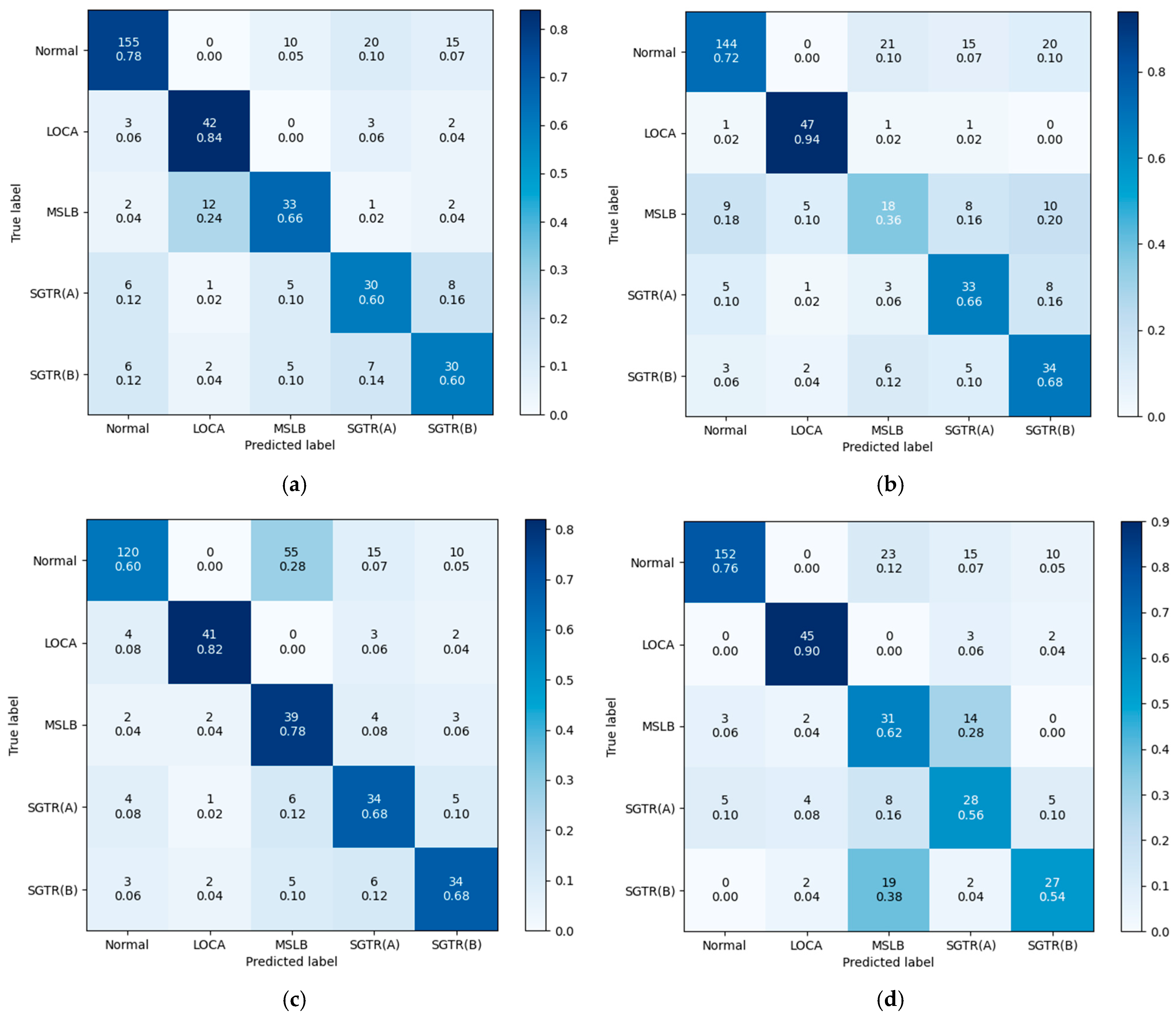
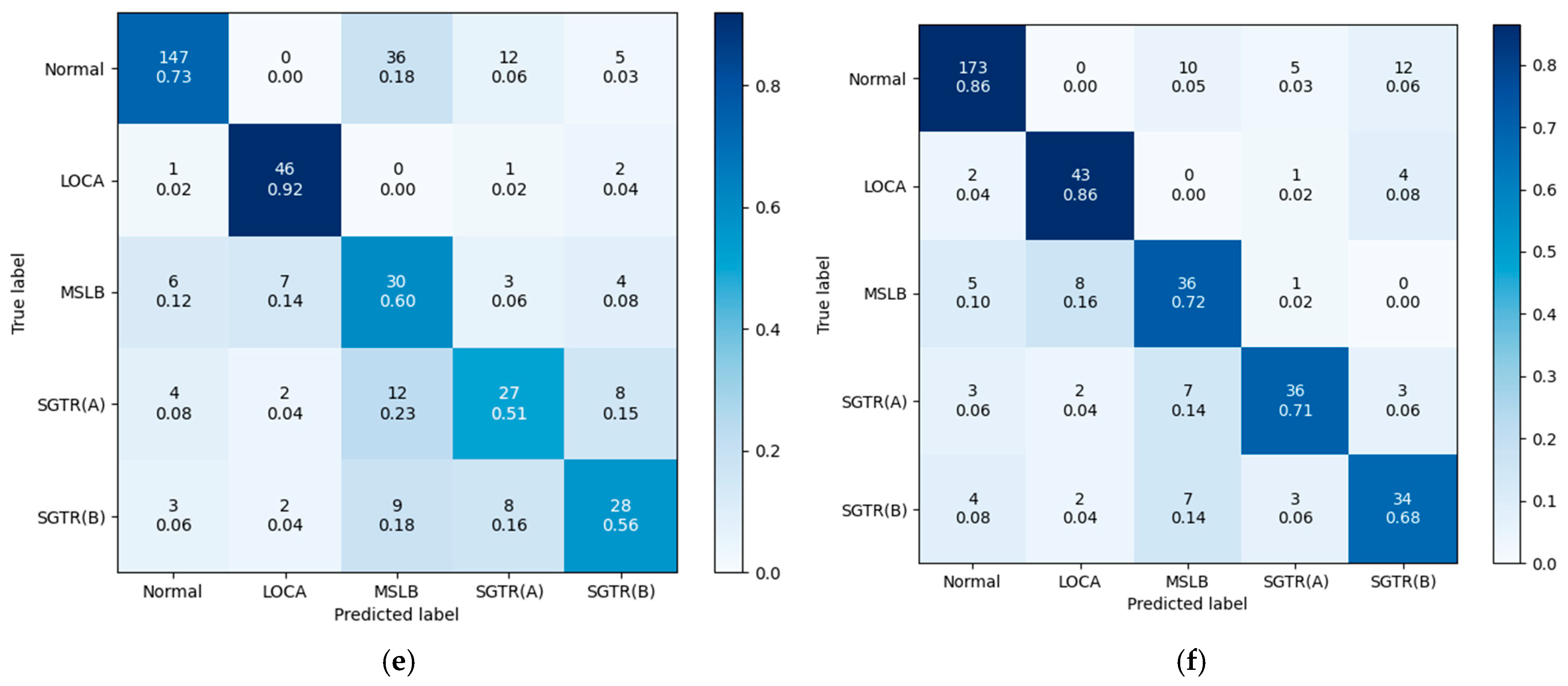
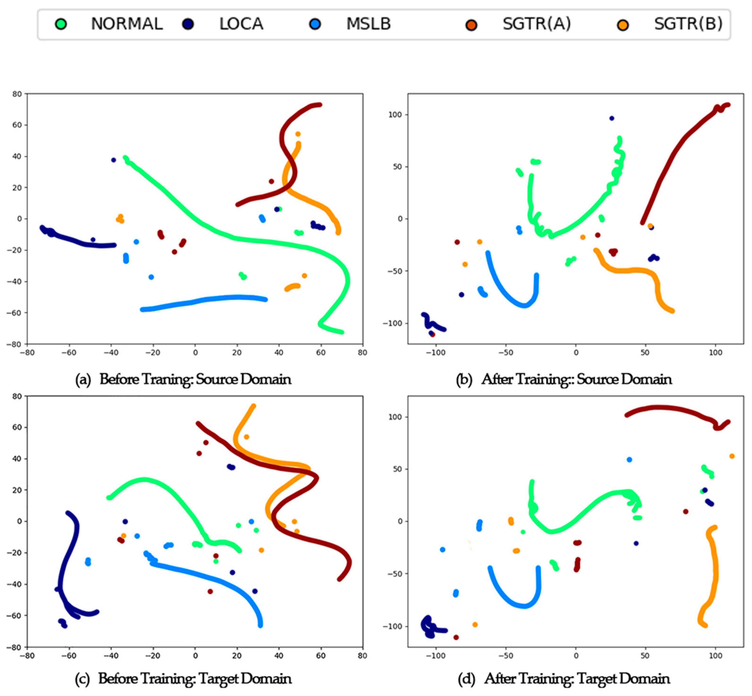
3.4. Evaluation Metrics and t-SNE Visualization

The main evaluation metrics for the experiment include the following: accuracy, macro-F1, minority-class recall, and AUC-ROC. Accuracy measures the overall correctness of predictions. Macro-F1 and minority recall are used to assess the model’s ability to handle class imbalance, especially for rare fault types. AUC-ROC captures the model’s overall discriminative ability regardless of the decision threshold.

The corresponding definitions are as follows:

Accuracy:

$$\mathrm{Accuracy}={\displaystyle \frac{TP+TN}{TP+TN+FP+FN}}$$

(27)

TP, TN, FP, and FN mean true positives, true negatives, false positives, and false negatives, respectively.

Macro-F1:

$$\mathrm{MacroF}1={\displaystyle \frac{1}{C}}{\displaystyle \sum _{i=1}^C\frac{2P_i{R}_i}{P_i+R_i}}$$

(28)

C is the total number of classes, $P_i={\displaystyle \frac{T{P}_i}{T{P}_i+F{P}_i}}$, $R_i={\displaystyle \frac{T{P}_i}{T{P}_i+F{N}_i}}$.

Minority-class recall:

$${\mathrm{Recall}}_{\mathrm{minor}}={\displaystyle \frac{T{P}_{\mathrm{minor}}}{T{P}_{\mathrm{minor}}+F{N}_{\mathrm{minor}}}}$$

(29)

AUC-ROC:

$$\mathrm{AUC}={\displaystyle {\int }_0^1\mathrm{TPR}}(t)d(\mathrm{FPR}(t))$$

(30)

$$\mathrm{TPR}={\displaystyle \frac{TP}{TP+FN}}$$

(31)

$$\mathrm{FPR}={\displaystyle \frac{FP}{FP+TN}}$$

(32)

We also provide a t-SNE comparison plot to visually compare the 2D feature distributions of the source and target domains before and after training.

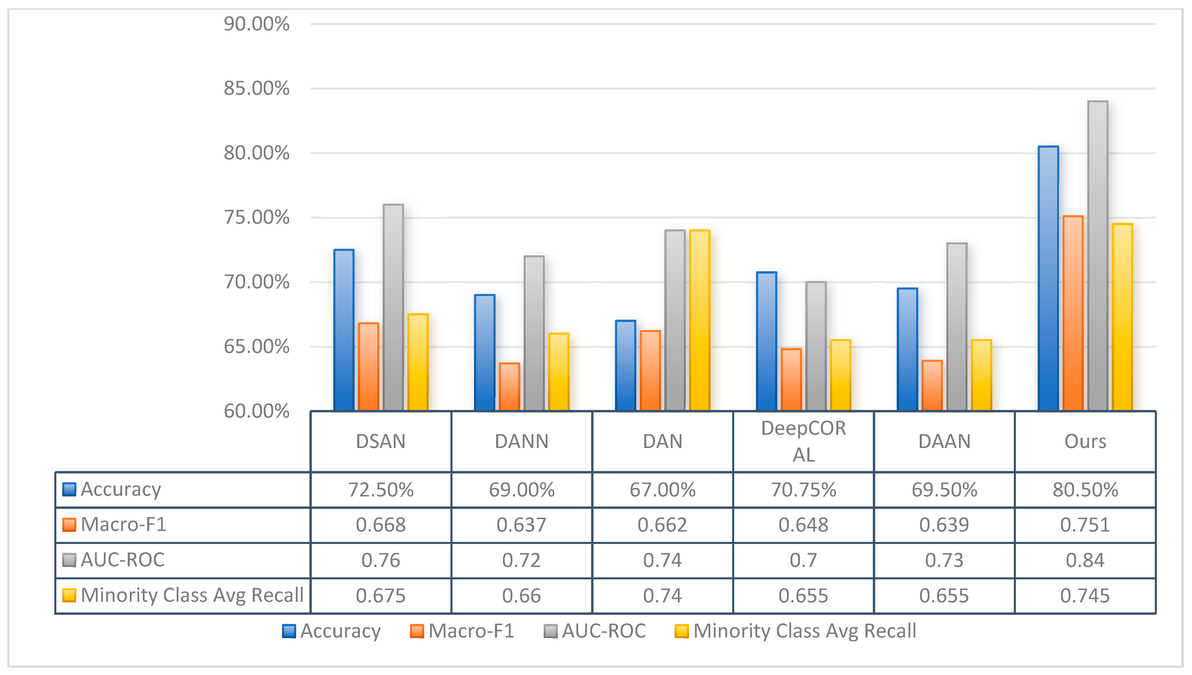
3.5. Results and Discussion

Figure 3 and Figure 4 show the comparisons of various metrics for the six models mentioned above, and the corresponding confusion matrices, respectively.

In terms of overall accuracy, the DSAN and DeepCORAL perform relatively similarly, with accuracies of 72.5% and 70.75%, respectively, slightly outperforming other traditional transfer learning models such as the DANN, DAN, and DAAN. This indicates that these two models have certain advantages in terms of overall classification ability under small-sample and class-imbalance conditions. The improved DSAN performs the best, with an 8.0% improvement over the DSAN’s overall accuracy, clearly outperforming other models. This demonstrates that the model has significantly improved its overall classification ability compared to traditional models.

In terms of minority-class recall analysis, the classification accuracy of the LOCA class remains stable across all methods, with high distinguishability in each method. The categories MSLB, SGTR (A), and SGTR (B) show more balanced classification in the improved DSAN, with a reduced number of misclassifications compared to other methods. This suggests that the improved model better adapts to the minority class, demonstrating the model’s ability to more precisely define boundaries between multiple classes.

The improved DSAN and DAN achieve average recall rates for the minority classes of 74.5% and 74.0%, respectively, indicating that both models have high prediction accuracy for the minority classes.

AUC-ROC represents the area under the receiver operating characteristic curve, which measures the model’s classification ability at different thresholds. The closer the AUC value is to 1, the better the model’s performance. In terms of the AUC-ROC, the improved DSAN achieves 84%, far surpassing the DSAN’s 76.0%, indicating that it can more accurately distinguish between positive and negative classes.

Compared to the original DSAN method, the improved DSAN shows performance improvements in classification across all categories:

The classification results show consistent improvements across multiple categories. Specifically, the correct predictions for the NORMAL class increased from 77.5% to 86.5%, while the MSLB class improved from 66.0% to 72.0%. For the SGTR (A) class, the accuracy rose from 60.0% to 72.0%, and for SGTR (B), from 60.0% to 68.0%, demonstrating a notable enhancement. In all cases, misclassifications were reduced, indicating that the proposed method effectively enhances class-specific recognition performance.

The improved DSAN outperforms other methods in classification accuracy for the NORMAL, MSLB, SGTR (A), and SGTR (B) classes, with a significant decrease in misclassification rates.

Furthermore, we performed t-SNE visualization of the feature distributions in the source and target domains before and after training with the improved DSAN model, as shown in Figure 5.

• Before Training (plots a and c):

Source Domain (plot a): Before transfer learning, the feature distribution in the source domain shows significant class overlap, particularly between the SGTR (A) and SGTR (B) conditions, indicating that the features are not fully separable. This overlap makes it difficult for the classification model to effectively distinguish between different fault types, as seen in the t-SNE plot where the feature samples of different classes are scattered in a disorganized manner.

Target Domain (plot c): Similarly, in the target domain, different fault types exhibit significant mixing, with blurred boundaries between classes, causing the features to be more compact and harder to distinguish in the feature space.

• After Training (plots b and d):

Source Domain (plot b): After applying transfer learning, the feature distribution in the source domain becomes more spread out, and the boundaries between different fault types become clearer. This indicates that transfer learning techniques, such as feature adaptation and domain alignment, have effectively optimized the feature distribution in the source domain, making the features more distinguishable.

Target Domain (plot d): The improvement in the target domain is particularly notable. The t-SNE visualization after transfer learning shows that the distribution of different classes in the target domain has become more distinct, and the overlap between classes has significantly decreased. Compared to the pre-transfer learning plots (plots a and c), plots b and d show substantial domain alignment.

These results demonstrate that the WFL and CPC significantly enhanced the learning ability of minority class samples, reduced the interference from erroneous pseudo-labels, improved fault classification performance, and reduced the domain discrepancy.

3.6. Ablation Experiments and Results Analysis

This section primarily uses ablation experiments to discuss and validate the model’s hyperparameter settings and the contribution of each component, including the choice of γ in the WFL, the individual and combined benefits of WFL and CPC, and the performance of GAF image transformation compared to other methods on the same dataset.

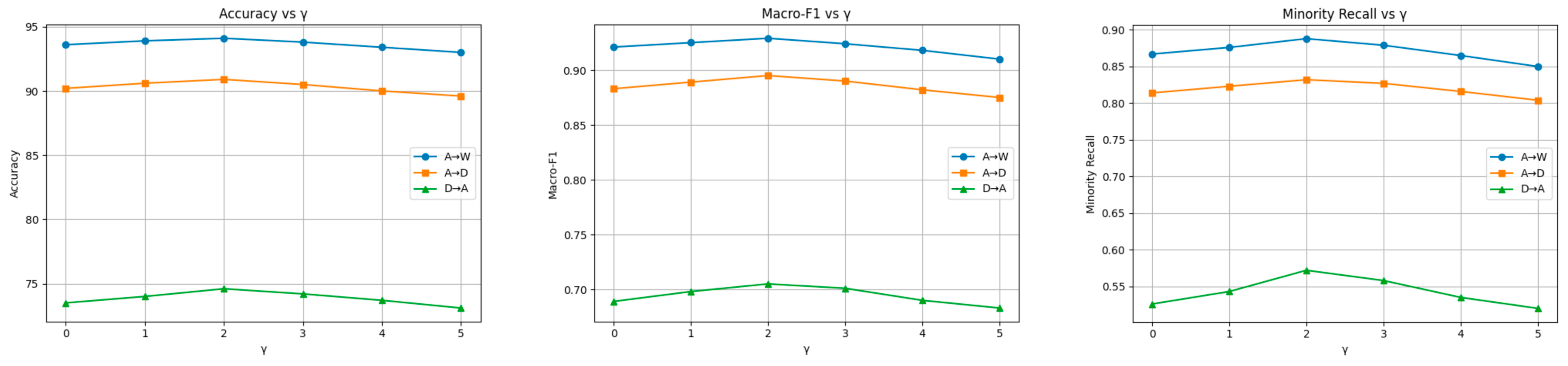
3.6.1. The Choice of γ

To determine the most suitable γ for the WFL, we validate a DSAN variant augmented only with WFL on the Office-31 dataset. In our experiments, γ is swept from 0 to 5—note that when γ = 0, the WFL reverts to the original DSAN loss, yielding the unmodified DSAN model.

Office-31 [44] is a benchmark dataset for domain adaptation, comprising 4110 images in 31 classes collected from three distinct domains: Amazon (A), which contains images downloaded from amazon.com, and Webcam (W) and DSLR (D), which contain images taken by a Web camera and digital SLR camera with different photographic settings. Office-31 itself inherently exhibits class imbalance, with some of its 31 categories represented by far fewer images than others.

As shown in Figure 6, the focusing parameter γ is observed in the WFL increases from 0 (equivalent to standard cross-entropy) to 5, and the accuracy, macro-F1, and minority-class recall all improve simultaneously across the A→W, A→D, and D→A transfer tasks, reaching their joint maximum at γ = 2 (with an overall accuracy of 94.1%, 90.9%, and 74.6%, respectively; macro-F1 gains of 0.8–1.6 percentage points; and minority recall up by as much as 4.6 percentage points). Beyond γ = 2, these metrics begin to decline, indicating that an overly strong focusing factor excessively down-weights easy samples and magnifies noise. Therefore, γ = 2 achieves the optimal balance between suppressing easy examples and emphasizing hard ones, delivering the best minority-class performance without compromising overall accuracy.

3.6.2. Weight Focal Loss and Confidence-Based Pseudo-Label Calibration

As Section 2.4 describes, this work introduces WFL and CPC into the original DSAN, aiming at prioritizing minority-class samples and mitigating pseudo-label noise.

To quantify the individual and joint contributions of WFL and CPC, we evaluate these improvements on the Office-31 dataset. Eight ablation configurations are designed on three transfer tasks (A→W, A→D, and D→A):

1. Baseline: original DSAN (no WFL and no CPC);

2. DSAN + WFL only;

3–6. DSAN + CPC only with fixed thresholds (T = 0.5, 0.6, 0.7, and 0.8);

7. DSAN + CPC with variable range (T in [0.8, 0.5]);

8. DSAN + WFL + CPC with variable range (T in [0.8, 0.5]).

Table 3. Ablation study of WFL and CPC on DSAN performance across three Office-31 transfer tasks.

G R O U P	Method		A→W			A→D			D→A
	+WFL	+CPC (T)	Accuracy (%)	Macro-F1	Minority Recall	Accuracy (%)	Macro-F1	Minority Recall	Accuracy (%)	Macro-F1	Minority Recall
1	×	—	93.6	92.1	86.7	90.2	88.3	81.4	73.5	68.9	52.6
2	√	—	94.1	92.9	88.8	90.9	89.5	83.2	74.6	70.5	57.2
3	×	0.5	91.8	89.5	86.0	88.5	86.2	79.5	70.2	65.2	53.5
4	×	0.6	92.1	89.8	86.5	88.7	86.5	80.2	70.6	65.6	54.5
5	×	0.7	92.5	90.3	86.8	89.2	86.9	80.8	71.3	66.2	55.0
6	×	0.8	92.8	90.7	86.5	89.5	87.2	80.5	71.8	66.8	55.2
7	×	0.8~0.5	94.0	92.8	88.7	90.8	89.4	83.0	75.0	70.9	57.4
8	√	0.8~0.5	94.3	93.3	89.2	91.1	89.9	84.0	75.4	71.5	58.2

summarizes the accuracy, macro-F1, and minority-class recall achieved under each configuration. This is summarized as follows:

In eight ablation configurations on the three Office-31 transfer tasks (A→W, A→D, and D→A), we observe that introducing WFL alone significantly boosts minority-class sensitivity and overall performance (e.g., accuracy on A→W rises from 93.6% to 94.1%, and minority recall from 86.7% to 88.8%). Using CPC alone—within T ∈ [0.8, 0.5]—improves minority recall but yields only modest macro-F1 gains. When both methods are combined, the model attains its best results on all tasks—A→W (accuracy 94.3%, macro-F1 93.3%, and minority recall 89.2%), A→D (91.1%, 89.9%, and 84.0%), and D→A (75.4%, 71.5%, and 58.2%)—with average improvements of approximately +0.7% in accuracy, +1.5% in macro-F1, and +2.5% in minority recall. These results confirm the synergistic benefit of WFL and CPC.

3.6.3. GAF and Pseudo-Color Mapping

To evaluate the role of the image transformation module in the proposed fault diagnosis framework, we conducted ablation experiments comparing four image generation strategies based on NPPAD and AP-1000: GAF with pseudo-color mapping, recurrence plot (RP), Continuous Wavelet Transform (CWT), and grayscale GAF without pseudo-color. This was done while keeping the feature selection, network architecture, and training strategy unchanged. As shown in

Table 4. Performance comparison of time-series image encoding methods (GAF, RP, CWT and pseudo-colored GAF).

Method	Accuracy (%)	Macro-F1	AUC-ROC	Minority Recall
GAF+pseudo-color	80.5	0.751	0.84	0.745
RP	76.8	0.715	0.82	0.780
CWT	79.2	0.740	0.83	0.735
GAF	78.0	0.720	0.81	0.700

, each method was assessed using the accuracy, macro-F1, AUC-ROC, and minority recall.

The results show that the GAF with pseudo-color mapping achieves the best overall performance by effectively capturing global temporal structures while enhancing texture information for deep models. In contrast, the RP method improves minority-class recall but lowers overall accuracy due to its sensitivity to repetitive patterns. CWT provides good time–frequency resolution and performs comparably to GAF, but is slightly inferior in modeling global dependencies. Grayscale GAF yields the lowest performance, indicating that pseudo-color mapping significantly enhances the model’s discriminative capacity.

These findings confirm that the choice of image transformation strategy significantly impacts classification performance. The combination of GAF’s structured temporal encoding and pseudo-color enhancement prove essential to the proposed framework, enabling the model to maintain high overall accuracy while effectively identifying minority-class faults.

3.7. Assessment of Online Deployability

To evaluate the inference efficiency of the proposed diagnostic framework, we processed the entire dataset, containing 600 source-domain and 400 target-domain samples, and measured the execution time of each component in the test pipeline. The pipeline includes feature extraction, time-series to image transformation (using GAF), pseudo-color mapping, model inference, and output generation.

Based on the runtime statistics collected over all 1000 samples, the average processing time per sample was, approximately, as follows: 2.5 ms for feature extraction, 6.0 ms for image transformation, 3.0 ms for pseudo-color mapping, 9.6 ms for model inference, and 0.5 ms for output writing, totaling around 21.6 ms per sample. Thus, the total inference time for the full dataset was approximately 21.6 s.

It should be noted that these measurements were obtained under an offline deployment setting, where all processes were executed locally without any network communication or real-time data acquisition. Hence, the current study remains limited in addressing the practical considerations of online deployment, which warrants further investigation in future work.

4. Conclusions and Future Work

Existing transfer learning models, such as the DANN, DAN, DeepCORAL, and DAAN, primarily focus on aligning the global distributions between the source and target domains, while neglecting intra-domain feature alignment. This limitation hinders their ability to capture fine-grained class-specific features, which is particularly problematic in fault diagnosis tasks where distinguishing subtle differences is crucial. Although the DSAN model strengthens intra-domain alignment, it, like the aforementioned models, performs poorly in handling class imbalance. These models tend to favor the majority class, leading to suboptimal performance in classifying the minority class, which is particularly critical in fault diagnosis tasks. Furthermore, these models are prone to overfitting in small-sample scenarios, lacking sufficient generalization ability, which diminishes their practical effectiveness in data-scarce environments. Additionally, models relying on pseudo-labeling are susceptible to pseudo-label noise, especially when true labels are absent in the target domain. Incorrect pseudo-labels negatively impact the model’s learning process, reducing its performance.

To address these issues, this study presents a fault diagnosis framework for pressurized water reactors. By integrating key parameter selection via SDG, GAF-based time-series transformation, and an enhanced DSAN model with WFL and CPC, the proposed framework raises the overall accuracy from 72.5% to 80.5%, increases macro-F1 to 0.75 and AUC-ROC to 0.84, and improves average minority-class recall to 74.5%, outperforming the original DSAN and four baselines by explicitly prioritizing minority-class samples and mitigating pseudo-label noise. It shows significant advantages in multi-class classification tasks, especially under conditions of small sample sizes and class imbalance, indicating that the WFL and CPC strategies effectively enhance the model’s classification ability. Through the ablation study, we observe that the model achieves optimal performance when the focusing parameter γ is set to 2 and the pseudo-label confidence threshold gradually decreases from 0.8 to 0.5.

From the perspective of minority-class recall and classification performance, the proposed method still has some limitations, suggesting that the classification performance of minority classes may still be affected by pseudo-label noise, target domain class bias, insufficient domain alignment, and computational complexity. Future work may focus on improving fault diagnosis performance by exploring more robust pseudo-label self-correction methods, optimizing domain alignment with adversarial learning, and enhancing class balancing strategies.

References

1. Qi, B.; Liang, J.; Tong, J. Fault Diagnosis Techniques for Nuclear Power Plants: A Review from the Artificial Intelligence Perspective. Energies 2023, 16, 1850. [Google Scholar] [CrossRef]
2. Min, J.H.; Kim, D.-W.; Park, C.-Y. Demonstration of the Validity of the Early Warning in Online Monitoring System for Nuclear Power Plants. Nucl. Eng. Des. 2019, 349, 56–62. [Google Scholar] [CrossRef]
3. Li, X.; Fu, X.-M.; Xiong, F.-R.; Bai, X.-M. Deep Learning-Based Unsupervised Representation Clustering Methodology for Automatic Nuclear Reactor Operating Transient Identification. Knowl. Based Syst. 2020, 204, 106178. [Google Scholar] [CrossRef]
4. Yue, P.; Fang, F.; Xu, P.; Xie, H.; Duan, Q.; Lin, J.; Xie, L. Noise Resistant Steam Generator Water Level Reconstruction for Nuclear Power Plant Based on Deep Residual Shrinkage Network. Ann. Nucl. Energy 2023, 193, 110038. [Google Scholar] [CrossRef]
5. Tonday Rodriguez, J.C.; Perry, D.; Rahman, M.A.; Alam, S.B. An Intelligent Hierarchical Framework for Efficient Fault Detection and Diagnosis in Nuclear Power Plants. In Proceedings of the Sixth Workshop on CPS&IoT Security and Privacy, Salt Lake City, UT, USA, 18 October 2024; Association for Computing Machinery: New York, NY, USA, 2024; pp. 80–92. [Google Scholar] [CrossRef]
6. Xu, Y.; Cai, Y.; Song, L. Review of Research on Condition Assessment of Nuclear Power Plant Equipment Based on Data-Driven. J. Shanghai Jiaotong Univ. 2022, 56, 267–278. [Google Scholar] [CrossRef]
7. Guo, J.; Wang, Y.; Sun, X.; Liu, S.; Du, B. Imbalanced Data Fault Diagnosis Method for Nuclear Power Plants Based on Convolutional Variational Autoencoding Wasserstein Generative Adversarial Network and Random Forest. Nucl. Eng. Technol. 2024, 56, 5055–5067. [Google Scholar] [CrossRef]
8. Yin, W.; Xia, H.; Huang, X.; Wang, Z. A Fault Diagnosis Method for Nuclear Power Plants Rotating Machinery Based on Deep Learning under Imbalanced Samples. Ann. Nucl. Energy 2024, 199, 110340. [Google Scholar] [CrossRef]
9. Li, G.; Li, Y.; Li, S.; Sun, S.; Wang, H.; Zhao, J.; Sun, B.; Shi, J. Self-Improving Few-Shot Fault Diagnosis for Nuclear Power Plant Based on Man-Machine Collaboration. Nucl. Eng. Des. 2024, 420, 113051. [Google Scholar] [CrossRef]
10. Dai, Y.; Peng, L.; Juan, Z.; Liang, Y.; Shen, J.; Wang, S.; Tan, S.; Yu, H.; Sun, M. An Intelligent Fault Diagnosis Method for Imbalanced Nuclear Power Plant Data Based on Generative Adversarial Networks. J. Electr. Eng. Technol. 2023, 18, 3237–3252. [Google Scholar] [CrossRef]
11. Li, J.; Lin, M.; Li, Y.; Wang, X. Transfer Learning with Limited Labeled Data for Fault Diagnosis in Nuclear Power Plants. Nucl. Eng. Des. 2022, 390, 111690. [Google Scholar] [CrossRef]
12. Zhuang, F.; Qi, Z.; Duan, K.; Xi, D.; Zhu, Y.; Zhu, H.; Xiong, H.; He, Q. A Comprehensive Survey on Transfer Learning. Proc. IEEE 2021, 109, 43–76. [Google Scholar] [CrossRef]
13. Pan, S.J.; Tsang, I.W.; Kwok, J.T.; Yang, Q. Domain Adaptation via Transfer Component Analysis. IEEE Trans. Neural Netw. 2011, 22, 199–210. [Google Scholar] [CrossRef] [PubMed]
14. Long, M.; Wang, J.; Ding, G.; Sun, J.; Yu, P.S. Transfer Feature Learning with Joint Distribution Adaptation. In Proceedings of the 2013 IEEE International Conference on Computer Vision, Sydney, Australia, 1–8 December 2013; pp. 2200–2207. [Google Scholar] [CrossRef]
15. Ganin, Y.; Ustinova, E.; Ajakan, H.; Germain, P.; Larochelle, H.; Laviolette, F.; Marchand, M.; Lempitsky, V. Domain-Adversarial Training of Neural Networks. In Domain Adaptation in Computer Vision Applications; Csurka, G., Ed.; Springer International Publishing: Cham, Switzerland, 2017; pp. 189–209. ISBN 978-3-319-58347-1. [Google Scholar]
16. Zhu, J.-Y.; Park, T.; Isola, P.; Efros, A.A. Unpaired Image-to-Image Translation Using Cycle-Consistent Adversarial Networks. In Proceedings of the 2017 IEEE International Conference on Computer Vision (ICCV), Venice, Italy, 22–29 October 2017; pp. 2242–2251. [Google Scholar] [CrossRef]
17. Zhu, Y.; Zhuang, F.; Wang, J.; Ke, G.; Chen, J.; Bian, J.; Xiong, H.; He, Q. Deep Subdomain Adaptation Network for Image Classification. IEEE Trans. Neural Netw. Learn. Syst. 2021, 32, 1713–1722. [Google Scholar] [CrossRef] [PubMed]
18. Liu, J.; Zhang, Q.; Macián-Juan, R. Enhancing Interpretability in Neural Networks for Nuclear Power Plant Fault Diagnosis: A Comprehensive Analysis and Improvement Approach. Prog. Nucl. Energy 2024, 174, 105287. [Google Scholar] [CrossRef]
19. Park, J.H.; Jo, H.S.; Lee, S.H.; Oh, S.W.; Na, M.G. A Reliable Intelligent Diagnostic Assistant for Nuclear Power Plants Using Explainable Artificial Intelligence of GRU-AE, LightGBM and SHAP. Nucl. Eng. Technol. 2022, 54, 1271–1287. [Google Scholar] [CrossRef]
20. Liu, Y.-K.; Wu, G.-H.; Xie, C.-L.; Duan, Z.-Y.; Peng, M.-J.; Li, M.-K. A Fault Diagnosis Method Based on Signed Directed Graph and Matrix for Nuclear Power Plants. Nucl. Eng. Des. 2016, 297, 166–174. [Google Scholar] [CrossRef]
21. Chen, G.; Yang, Z.; Sun, J. Applying Bayesian Networks in Nuclear Power Plant Safety Analysis. Procedia Eng. 2010, 7, 81–87. [Google Scholar] [CrossRef]
22. Bensi, M.T.; Groth, K.M. On the Value of Data Fusion and Model Integration for Generating Real-Time Risk Insights for Nuclear Power Reactors. Prog. Nucl. Energy 2020, 129, 103497. [Google Scholar] [CrossRef]
23. Pan, S.J.; Yang, Q. A Survey on Transfer Learning. IEEE Trans. Knowl. Data Eng. 2010, 22, 1345–1359. [Google Scholar] [CrossRef]
24. Wang, Z.; Oates, T. Imaging Time-Series to Improve Classification and Imputation 2015. arXiv 2015, arXiv:1506.00327. [Google Scholar]
25. Qi, B.; Xiao, X.; Liang, J.; Po, L.C.; Zhang, L.; Tong, J. An Open Time-Series Simulated Dataset Covering Various Accidents for Nuclear Power Plants. Sci. Data 2022, 9, 766. [Google Scholar] [CrossRef] [PubMed]
26. Das, S.; Pan, I.; Das, S. Fractional Order Fuzzy Control of Nuclear Reactor Power with Thermal-Hydraulic Effects in the Presence of Random Network Induced Delay and Sensor Noise Having Long Range Dependence. Energy Convers. Manag. 2013, 68, 200–218. [Google Scholar] [CrossRef]
27. Peng, Z.; Zhang, K.; Chai, Y. Multiple Fault Diagnosis for Hydraulic Systems Using Nearest-Centroid-with-DBA and Random-Forest-Based-Time-Series-Classification. In Proceedings of the 2020 39th Chinese Control Conference (CCC), Shenyang, China, 27–30 July 2020; pp. 29–86. [Google Scholar]
28. Chae, Y.H.; Kim, S.G.; Choi, J.; Koo, S.R.; Kim, J. Enhancing Nuclear Power Plant Diagnostics: A Comparative Analysis of XAI-Based Feature Selection Methods for Abnormal and Emergency Scenario Detection. Prog. Nucl. Energy 2025, 185, 105759. [Google Scholar] [CrossRef]
29. Wu, G.; Yuan, D.; Yin, J.; Xiao, Y.; Ji, D. A Framework for Monitoring and Fault Diagnosis in Nuclear Power Plants Based on Signed Directed Graph Methods. Front. Energy Res. 2021, 9, 641545. [Google Scholar] [CrossRef]
30. Diao, X.; Zhao, Y.; Pietrykowski, M.; Wang, Z.; Bragg-Sitton, S.; Smidts, C. Fault Propagation and Effects Analysis for Designing an Online Monitoring System for the Secondary Loop of the Nuclear Power Plant Portion of a Hybrid Energy System. Nucl. Technol. 2018, 202, 106–123. [Google Scholar] [CrossRef]
31. Liu, Y.; Abiodun, A.; Wen, Z.; Wu, M.; Peng, M.; Yu, W. A Cascade Intelligent Fault Diagnostic Technique for Nuclear Power Plants. J. Nucl. Sci. Technol. 2018, 55, 254–266. [Google Scholar] [CrossRef]
32. Selvapriya, B.; Raghu, B. Pseudocoloring of Medical Images: A Research. Int. J. Eng. Adv. Technol. 2019, 8, 3712–3716. [Google Scholar] [CrossRef]
33. Yosinski, J.; Clune, J.; Bengio, Y.; Lipson, H. How Transferable Are Features in Deep Neural Networks? In Advances in Neural Information Processing Systems 27 (NIPS 2014), Proceedings of the 28th Annual Conference on Neural Information Processing Systems 2014, Montreal, QC, Canada, 8–13 December 2014; Neural Information Processing Systems Foundation, Inc. (NeurIPS): La Jolla, CA, USA, 2015. [Google Scholar]
34. Wang, Z.; Oates, T. Encoding Time Series as Images for Visual Inspection and Classification Using Tiled Convolutional Neural Networks. In Proceedings of the Workshops at the Twenty-Ninth AAAI Conference on Artificial Intelligence, Austin, TX, USA, 25–30 January 2015. [Google Scholar]
35. Hatami, N.; Gavet, Y.; Debayle, J. Classification of Time-Series Images Using Deep Convolutional Neural Networks. In Proceedings of the Tenth International Conference on Machine Vision (ICMV 2017), Vienna, Austria, 13–15 November 2017. [Google Scholar]
36. Lu, J.; Wang, K.; Chen, C.; Ji, W. A Deep Learning Method for Rolling Bearing Fault Diagnosis Based on Attention Mechanism and Graham Angle Field. Sensors 2023, 23, 5487. [Google Scholar] [CrossRef]
37. Styan, G.P.H. Hadamard Products and Multivariate Statistical Analysis. Linear Algebra Its Appl. 1973, 6, 217–240. [Google Scholar] [CrossRef]
38. LeCun, Y.; Bottou, L.; Orr, G.B.; Müller, K.-R. Efficient BackProp. In Neural Networks: Tricks of the Trade; Montavon, G., Orr, G.B., Müller, K.-R., Eds.; Springer: Berlin/Heidelberg, Germany, 1998; Volume 1524, pp. 9–50. [Google Scholar] [CrossRef]
39. Le, D.N.T.; Le, H.X.; Ngo, L.T.; Ngo, H.T. Transfer Learning with Class-Weighted and Focal Loss Function for Automatic Skin Cancer Classification 2020. arXiv 2020, arXiv:2009.05977. [Google Scholar]
40. Toba, M.; Uchida, S.; Hayashi, H. Pseudo-Label Learning with Calibrated Confidence Using an Energy-Based Model. arXiv 2024, arXiv:2404.09585v1. Available online: https://arxiv.org/html/2404.09585v1 (accessed on 19 April 2025).
41. Long, M.; Cao, Y.; Wang, J.; Jordan, M.I. Learning Transferable Features with Deep Adaptation Networks. In Proceedings of the 32nd International Conference on Machine Learning, Lille, France, 6–11 July 2015; Bach, F., Blei, D., Eds.; Proceedings of Machine Learning Research. Volume 37, pp. 97–105. [Google Scholar]
42. Sun, B.; Saenko, K. Deep CORAL: Correlation Alignment for Deep Domain Adaptation. In Computer Vision—ECCV 2016 Workshops, Part III; Hua, G., Jégou, H., Eds.; Lecture Notes in Computer Science; Springer: Cham, Switzerland, 2016; Volume 9915, pp. 443–450. [Google Scholar] [CrossRef]
43. Wen, J.; He, K.; Huo, J.; Gu, Z.; Gao, Y. Unsupervised Domain Attention Adaptation Network for Caricature Attribute Recognition. In Proceedings of the Computer Vision—ECCV 2020, Glasgow, UK, 23–28 August 2020; Vedaldi, A., Bischof, H., Brox, T., Frahm, J.-M., Eds.; Lecture Notes in Computer Science. Springer: Cham, Switzerland, 2020; Volume 12353, pp. 18–34. [Google Scholar] [CrossRef]
44. Saenko, K.; Kulis, B.; Fritz, M.; Darrell, T. Adapting Visual Category Models to New Domains. In Computer Vision—ECCV 2010; Daniilidis, K., Maragos, P., Paragios, N., Eds.; Springer: Berlin/Heidelberg, Germany, 2010; Volume 6314, pp. 213–226. [Google Scholar] [CrossRef]
Figure 1. Fault diagnosis framework based on an improved DSAN.
Energies 18 02334 g001
Figure 2. Fault propagation pathway (SDG model).
Energies 18 02334 g002
Figure 3. Comparison of various metrics for the six models.
Energies 18 02334 g003
Figure 4. Confusion matrices: (a) DSAN; (b) DANN; (c) DAN; (d) DeepCORAL; (e) DAAN; (f) ours.
Energies 18 02334 g004aEnergies 18 02334 g004b
Figure 5. t-SNE visualization of the feature distribution in the source and target domains before and after training (plots (ad)).
Energies 18 02334 g005
Figure 6. Impact of γ in WFL on accuracy, macro-F1, and minority-class recall across three transfer tasks (A→W, A→D, and D→A).
Energies 18 02334 g006