A Trading Model for the Electricity Spot Market That Takes into Account the Preference for Energy Storage Trading

Abstract

With the continuous expansion of new energy installed capacity, the flexible regulation role of energy storage in the electricity spot market is becoming more and more prominent. However, traditional trading models often ignore the multiple trading preferences of energy storage. In this paper, we propose an electricity spot market trading model that considers the trading preferences of energy storage to incentivize energy storage to participate more actively in the market. First, the trading preferences of energy storage are modeled with a utility function in which the time preference coefficient and price elasticity are introduced. Then, the utility function is embedded into the spot market clearing model to establish a two-tier model of the spot market, which maximizes social welfare in the upper tier and maximizes energy storage benefits in the lower tier. Finally, the model is solved using KKT and large M methods, and its effectiveness is evaluated on the IEEE39 node system and on a real grid in a specific region.

1. Introduction

With the transition of the global energy structure to a high proportion of renewable energy sources, power systems are facing the dual challenges of increased fluctuations in supply and demand and a shortage of flexible regulation resources [1]. Energy storage has become an important regulator of the new power system by virtue of its fast response and intertemporal energy transfer capability [2]. However, the participation of energy storage in the electricity spot market is still limited by multiple factors [3,4]. On the one hand, the current market mechanism does not match the physical characteristics of energy storage (e.g., charging and discharging efficiency, life decay) enough, which leads to limited arbitrage space; on the other hand, the storage operators present diversified trading preferences, covering non-economic objectives such as risk tolerance, new source consumption orientation, and equipment life preservation, and the traditional “revenue maximization” approach is not enough to meet these objectives. On the other hand, energy storage operators have diverse trading preferences (e.g., value-at-risk preference, new source consumption orientation, equipment lifetime preference), and the traditional “revenue maximization” model makes it difficult to portray such complex decision-making behaviors. In this context, it is of great theoretical and practical significance to construct an electric power spot market trading model that takes into account the trading preferences of energy storage operators to break the bottleneck of energy storage commercialization and to promote the safe and economic operation of the new electric power system.

Current studies on the preference of energy storage participation in spot market trading are mainly divided into preference modeling based on economic constraints and preference modeling based on technical constraints.

(1)

Preference modeling based on economic constraints of energy storage

Kazari et al. analyzed the impact of different types of energy storage on smoothing power fluctuations in the grid by establishing a clearing model for energy storage participation in the ancillary services market and compared the impacts of different storage charging and discharging rates on the market but did not take into account the impacts of storage revenue risk on transactions [5]. Wan et al. adjusted the electricity price by establishing an energy storage power prediction model, which ultimately guides the energy storage to participate in the market so as to smooth the power fluctuation more effectively, and elaborates the mechanism of the impact of the electricity price fluctuation on the transaction but does not take into account the storage’s own prediction of the electricity price [6]. Khani et al. established a capacity allocation model to optimize the allocation of energy storage based on the consideration of the benefits of energy storage participation in the standby auxiliary service market [7]. Farzin et al. proposed a scheduling model for energy storage participation in multiple scenarios, analyzed the impact of different scenarios on the benefits of energy storage, and described the trading preference of energy storage from the perspective of benefits but did not consider the charging and discharging preference of energy storage itself [8]. Fan et al. established a scheduling model for energy storage participation in the coordinated operation of the spot market and auxiliary service market and analyzed the trading preference of energy storage based on the revenue from the market perspective but did not consider the cyclic life preference of energy storage itself [9]. Peng et al. established a clearing model for energy storage participation in the spot market considering the uncertainty of electricity price, optimized the bidding strategy of energy storage participation in the market, and helped energy storage to participate in the market competition more actively, but did not take into account the preference of energy storage itself for the clearing price [10].

(2)

Preference modeling based on energy storage technology constraints

Li et al. modeled the wind power climbing scenario of the power system based on the event optimization theory and established a scheduling strategy model for energy storage to participate in the climbing market, smoothing the climbing rate of the power system. However, the benefits of energy storage participation in the market were not analyzed [11]. Li et al. established a trading model for VPP participation in the electricity spot market considering the lifetime cost of energy storage and proposed a preferred quantitative characterization method based on the cycle loss cost of energy storage, but it did not consider the difference in trading preferences between different types of energy storage [12]. He et al. established a trading model for energy storage participation in the FM auxiliary service market and analyzed the preference strategies of energy storage under different scenarios, but the analysis of the revenue situation of energy storage itself was insufficient [13]. David et al. established a day-ahead market and real-time market trading model considering the uncertainty of new energy output and analyzed the incentives of storage’s cycle life on trading but did not discuss the impact of storage’s revenue on trading under each scenario [14].

From the above studies, it can be seen that most of the existing studies consider economic constraints or technical constraints singly and analyze the trading preferences of energy storage in an incomplete way, which leads to the problems of insufficient release of the potential of energy storage, unfair distribution of social welfare, and so on.

This paper combines the theory of behavioral economics to portray the multiple trading preferences of energy storage and construct a two-layer trading model for its participation in the market and verifies the validity of the model in the IEEE39 node system and the actual power grid of a certain region. Compared with the traditional two-tier trading model, the model proposed in this paper takes into account the multi-dimensional trading preferences of energy storage, such as charging/discharging, offers, risk, cycle life, etc., and analyzes the mechanism of the impact of the trading preferences of energy storage on the trading from the point of view of the storage operator, which is of practical significance to enhance the efficiency of the market operation and stimulate the energy storage to participate in the market in a more proactive way.

2. Modeling of Energy Storage Preference Utility Functions

Energy storage trading preferences specifically refer to the decision-making preferences of energy storage operators when trading electricity, such as preferring to trade in a certain time period, or preferring high-risk, high-return trading strategies, or considering factors such as market rules and policy subsidies. Preferences are specifically modeled by weighing the utility of different factors and selecting the trading strategy with the greatest utility. However, trading preferences may not only be based on price differentials but may also involve a variety of factors such as risk, time, and policy.

The utility function is a central tool in economics to quantify the behavioral motivations of decision-making agents [15,16]. For energy storage, its trading preferences (e.g., time preference, price preference, risk preference, cycle count preference, etc.) directly affect the charging and discharging strategies, and the utility function transforms these preferences into mathematically optimizable forms.

2.1. Modeling of Charge and Discharge Time Preferences

The charging time preference weights are introduced in the utility function to enhance the charging and discharging behavior of the energy storage in a specific time period, which is modeled in the following equation:

$$U_k^t={\displaystyle \sum _{t\in T}({\tau }_{k,t}^{dis}{\lambda }_t{P}_{k,t}^{dis}-}{\tau }_{k,t}^{ch}{\lambda }_t{P}_{k,t}^{ch}),$$

(1)

where ${\tau }_{k,t}^{ch}$ and ${\tau }_{k,t}^{dis}$ are the preference weights (usually take values of 0~1), ${\lambda }_t$ is the real-time electricity price of the time period, and $P_{k,t}^{ch}$ and $P_{k,t}^{dis}$ are the charging and discharging power of the energy storage, respectively.

2.2. Modeling of Price Preferences

In order to quantify the dynamic response of the charging and discharging behavior of energy storage to real-time electricity prices, a price elasticity factor is introduced. The step-by-step modeling process is described as follows:

$$P_{k,t}^{ch}=\left\{\begin{array}{c}0\hfill \\ {\epsilon }_k^{ch}({\lambda }_k^t-{\lambda }_t)\hspace{1em}{\lambda }_k^{\min }\le {\lambda }_t\le {\lambda }_k^t\hfill \\ {\underset{¯}{P}}_k^{ch}\hspace{1em}\hspace{1em}\hspace{1em}\hspace{1em}{\lambda }_t<{\lambda }_k^{\min }\hfill \end{array}\right.,$$

(2)

$$P_{k,t}^{dis}=\left\{\begin{array}{c}0\hfill \\ {\epsilon }_k^{dis}({\lambda }_t-{\lambda }_k^t)\hspace{1em}{\lambda }_k^t\le {\lambda }_t\le {\lambda }_k^{\max }\hfill \\ {\underset{¯}{P}}_k^{dis}\hspace{1em}\hspace{1em}\hspace{1em}\hspace{1em}{\lambda }_t>{\lambda }_k^{\max }\hfill \end{array}\right.,$$

(3)

where ${\epsilon }_k^{ch}$ is the price elasticity coefficient; ${\lambda }_k^{\min }$ is the minimum price of electricity when the charging power reaches its maximum value ${\underset{¯}{P}}_k^{ch}$; and ${\lambda }_k^{\max }$ is the maximum price of electricity when the discharging power reaches its maximum value ${\underset{¯}{P}}_k^{dis}$.

In order to facilitate the solution of the above model in the trading model, the large M method [17] is commonly used to transform the segmented function into linear constraints as follows.

Charging constraints:

$${\lambda }_t-{\lambda }_k^t\le M(1-u_{k,t}^{ch})\hspace{1em}{u}_{k,t}^{ch}\in \{0,1\},$$

(4)

$$P_{k,t}^{ch}\le {\epsilon }_k^{ch}({\lambda }_k^{ch}-{\lambda }_t)+M(1-u_{k,t}^{ch}),$$

(5)

$$P_{k,t}^{ch}\ge {\epsilon }_k^{ch}({\lambda }_k^{ch}-{\lambda }_t)-M(1-u_{k,t}^{ch}),$$

(6)

$$P_{k,t}^{ch}\le {\underset{¯}{P}}_k^{ch}{u}_{k,t}^{ch}.$$

(7)

Discharge constraints:

$${\lambda }_t-{\lambda }_k^t\ge -M(1-u_{k,t}^{dis})\hspace{1em}{u}_{k,t}^{dis}\in \{0,1\},$$

(8)

$$P_{k,t}^{dis}\le {\epsilon }_k^{dis}({\lambda }_k^{dis}-{\lambda }_t)+M(1-u_{k,t}^{dis}),$$

(9)

$$P_{k,t}^{dis}\ge {\epsilon }_k^{dis}({\lambda }_k^{dis}-{\lambda }_t)-M(1-u_{k,t}^{dis}),$$

(10)

$$P_{k,t}^{dis}\le {\underset{¯}{P}}_k^{dis}{u}_{k,t}^{dis}.$$

(11)

Calibration of price elasticity coefficient: The price elasticity coefficient needs to be obtained through mathematical and statistical calculation using historical tariffs and storage charging and discharging records, as shown in the following formula:

$${\epsilon }_k^{ch}={\displaystyle \frac{1}{t}}{\displaystyle \sum _{t=1}^n\frac{\Delta P_{k,t}^{ch}}{\Delta ({\lambda }_{k,t}^{ch}-{\lambda }_{t,t})}}.$$

(12)

2.3. Modeling of Risk Appetite

In this paper, the modeling is achieved by introducing Conditional Value-at-Risk (CVaR) [18,19] to optimize the returns in the presence of risky scenarios, as follows:

$$CVa{R}_{\alpha }(R)=E\left\{R\right|R\le Va{R}_{\alpha }(R)\}={\displaystyle \frac{1}{\alpha }}{\displaystyle {\int }_0^{Va{R}_{\alpha }(R)}R}{\rho }_{R}dR\approx [VaR(R)+{\displaystyle \frac{1}{1+\alpha }}{\displaystyle \sum _{s\in S}{\pi }_{s}R]}.$$

(13)

where $R$ is the return on the random variable; $\alpha$ is the confidence level; ${\rho }_R$ is the cumulative probability density function of $R$; and ${\pi }_s$ is the scenario probability.

Introducing the dummy auxiliary variable $\phi$ and linearizing it yields the following:

$$CVaR(R)=\phi +{\displaystyle \frac{1}{1+\alpha }}{\displaystyle \sum _{s\in S}{\pi }_s{z}_s}.$$

(14)

Then, the optimization model of energy storage participation in market trading taking into account risk appetite can be expressed as follows:

$$\max \beta R+(1-\beta )(\phi +{\displaystyle \frac{1}{1+\alpha }}{\displaystyle \sum _{s\in S}{\pi }_s{z}_s)},$$

(15)

$$s.t.\{\begin{array}{l}{z}_n\ge 0\\ z_n\ge -R-\alpha \end{array},$$

(16)

where $\phi$ is the risk threshold; $z_s$ is the loss of revenue under the scenario s; and $\beta$ is the risk aversion coefficient ($\beta =0$ is perfect risk neutrality, while $\beta =1$ is extreme risk aversion).

2.4. Modeling of Charge–Discharge Cycle Count Preferences

Considering the impact of frequent charging and discharging of the energy storage on the lifetime, the cyclic lifetime loss cost is introduced in the following form:

$$C_k^{\mathrm{deg}}={\displaystyle \sum _{t,s}{\rho }_s(\frac{P_{k,t,s}^{ch}+P_{k,t,s}^{dis}}{2E_k}}{)}^{{\gamma }_k},$$

(17)

where ${\gamma }_k\ge 1$ is the lifetime decay index (usually takes values of 1.5~2).

3. Electricity Spot Market Trading Model Accounting for Storage Trading Preferences

In a spot market accounting for storage trading preferences, storage operators optimize their charging and discharging strategies based on the market price of electricity and express their trading preferences through utility functions and weighting coefficients. The two-layer game model consists of two interrelated layers: the upper-layer model minimizes the total cost of the power system or maximizes the social welfare and clears the real-time tariffs through the conditions of supply–demand balance, unit output, and transmission constraints; the lower-layer model focuses on the storage operators to optimize their charging and discharging strategies guided by the tariff signals and the objective function integrates the price-arbitrage gains, charging and discharging time preferences (e.g., peak discharge weights), risk aversion (e.g., peak discharge weights) and risk management (e.g., peak discharge weights). The objective function combines price arbitrage gain, charging and discharging time preference (e.g., peak discharge weight), risk avoidance (e.g., CVaR control), and cycle life loss cost (based on the equivalent number of charging and discharging times) and realizes the equilibrium interaction between tariffs and storage behaviors through the dynamic game to achieve the optimal trade-off between short-term market returns and long-term equipment sustainability.

In this paper, we refer to the trading rules of a regional electricity spot market in China in the modeling, assuming that energy storage acts as a price receiver (passive response to electricity price) or a strategic provider (active influence on electricity price) and only considers participating in the spot energy market while ignoring the auxiliary service market (typical application scenario: energy storage participates in the electricity energy market by arbitrage through the peak-valley price difference): the specific modeling process is described as follows.

3.1. Upper Level Modeling

The upper level establishes an objective function with the goal of maximizing social welfare,

$$\underset{{\lambda }_t,P_{i,t},P_{j,t}}{{\displaystyle \min }}{\displaystyle \sum _{t\in T}[}{\displaystyle \sum _{j\in D}{U}_j(P_{j,t})+{\displaystyle \sum _{i\in G}{C}_i(P_{i,t})]}},$$

(18)

where $U_j$ is the utility function on the user side; $C_i$ is the generation cost of the unit; and $P_{i,t}$ is the amount of electricity won.

Constraints

Node power balance:

$${\displaystyle \sum _{g\in G_i}{P}_{g,t}+P_{dis,t}-P_{ch,t}=D_{i,t}+{\displaystyle \sum _{l\in L_i}{P}_{l,t} (\forall i,t)}}.$$

(19)

Line capacity constraints:

$$-F_l^{\max }\le {\displaystyle \sum _{n}GSD{F}_{l,n}},$$

(20)

$$({\displaystyle \sum _{i\in G_n}{P}_{i,t}-{\displaystyle \sum _{j\in D_n}{P}_{j,t})\le F_l^{\max },\forall l,t}}.$$

(21)

The upper and lower limits of unit output are constrained as follows:

$$P_i^{\min }<P_{i,t}<P_i^{\max },\forall i,t,$$

(22)

$$P_j^{\min }\le P_{j,t}\le P_j^{\max },\forall j,t.$$

(23)

3.2. Lower-Level Modeling

Lower-tier storage has the goal of maximizing its own revenue while satisfying its own trading preferences,

$$\underset{P_{k,t}^{ch/dis},E_{k,t}}{\max }{\displaystyle \sum _{t\in T}[{\tau }_{k,t}^{dis}{\lambda }_t{P}_{k,t}^{dis}-}{\tau }_{k,t}^{ch}{\lambda }_t{P}_{k,t}^{ch}-{\beta }_k{\xi }_t-C_k^{\mathrm{deg}}].$$

(24)

Constraints

Energy storage charging and discharging power constraints:

$$0\le P_{k,t}^{ch}\le {\overline{P}}_k^{ch},$$

(25)

$$0\le P_{k,t}^{dis}\le {\overline{P}}_k^{dis}.$$

(26)

SOC state constraints:

$$E_{k,t+1}=E_{k,t}+{\eta }_k^{ch}{P}_{k,t}^{ch}-{\displaystyle \frac{1}{{\eta }_k^{dis}}}{P}_{k,t}^{dis}.$$

(27)

Capacity constraints:

$$E_k^{\min }\le E_{k,t}\le {\overline{E}}_k.$$

(28)

Trading preference constraints:

$$P_{k,t}^{ch}\le {\epsilon }_k^{ch}({\lambda }_k^{ch,t}-{\lambda }_t),$$

(29)

$$P_{k,t}^{dis}\le {\epsilon }_k^{dis}({\lambda }_t-{\lambda }_k^{dis,t}),$$

(30)

$${\xi }_t\ge \varsigma -({\lambda }_t{P}_{k,t}^{dis}-{\lambda }_t{P}_{k,t}^{ch})\hspace{1em}{\xi }_t\ge 0,\forall t.$$

(31)

3.3. Solving the Model

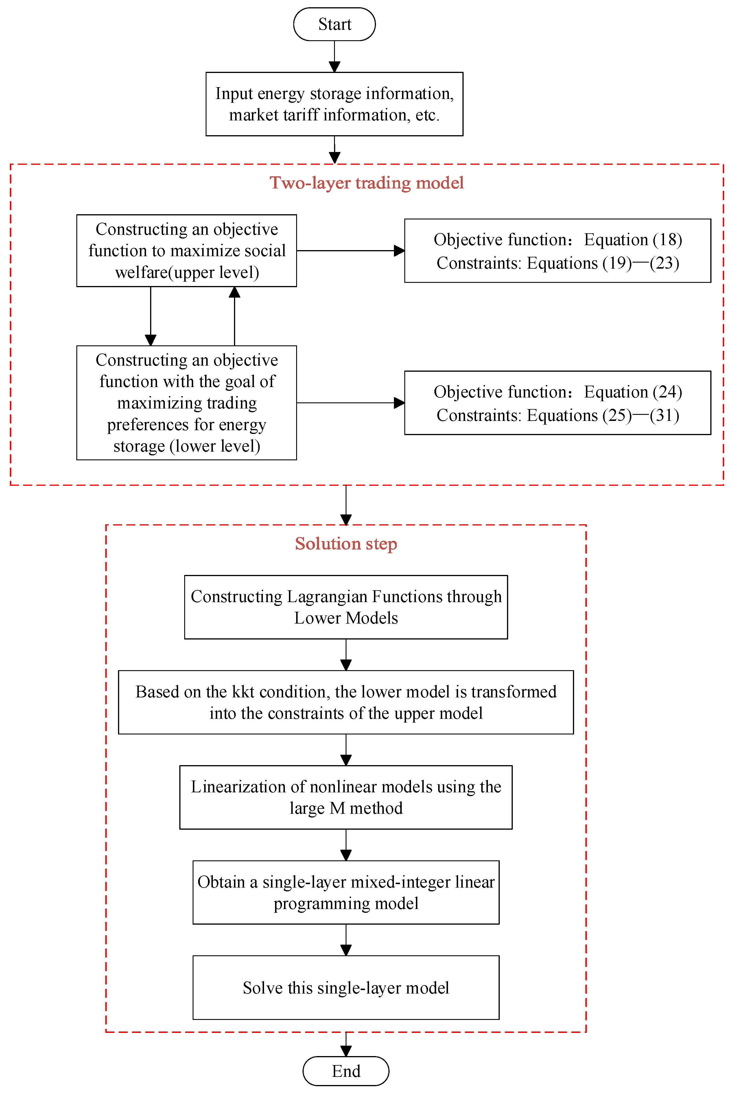
Due to the nested decision hierarchy of the two-tier trading model established in the previous section, the upper-tier decision affects the lower-tier strategy, which in turn reacts to the upper-tier objective function and constraints. This dynamic coupling leads to implicit dependencies between variables, which cannot be directly separated and handled by single-layer optimization methods. In the power market, the market price of electricity determines the charging and discharging strategies of energy storage, and the storage behavior changes the node injection power, which in turn affects the outcome of the electricity price clearing. This circular dependence makes the objective function and constraints show nonlinear interaction, which makes it difficult to directly solve the global optimal solution. Unable to carry out the solution directly, this paper adopts the KKT condition [20] to transform the lower model into the constraints of the upper model and then uses the large M method to eliminate the nonlinear terms for the solution; the flow chart of the algorithm is shown in Figure 1, and its derivation process is shown in the Appendix A.

4. Numerical Analysis

4.1. Single Typical Day Simulation Analysis

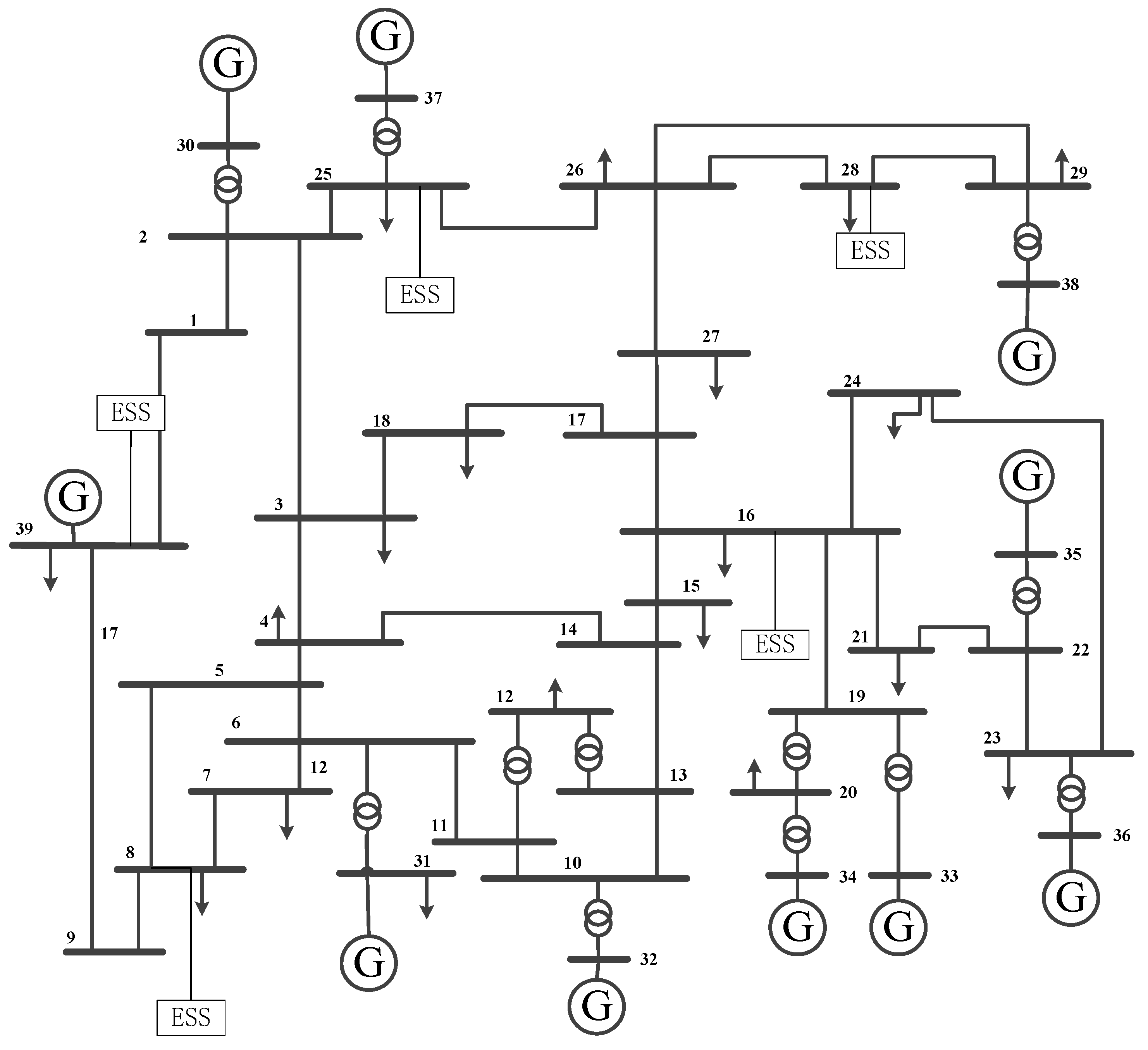
In this paper, the simulation analysis is based on the IEEE39 system as an example, which consists of 39 nodes, 10 generators, 46 transmission lines and 5 energy storage stations, and the system wiring diagram is shown in Figure 2.

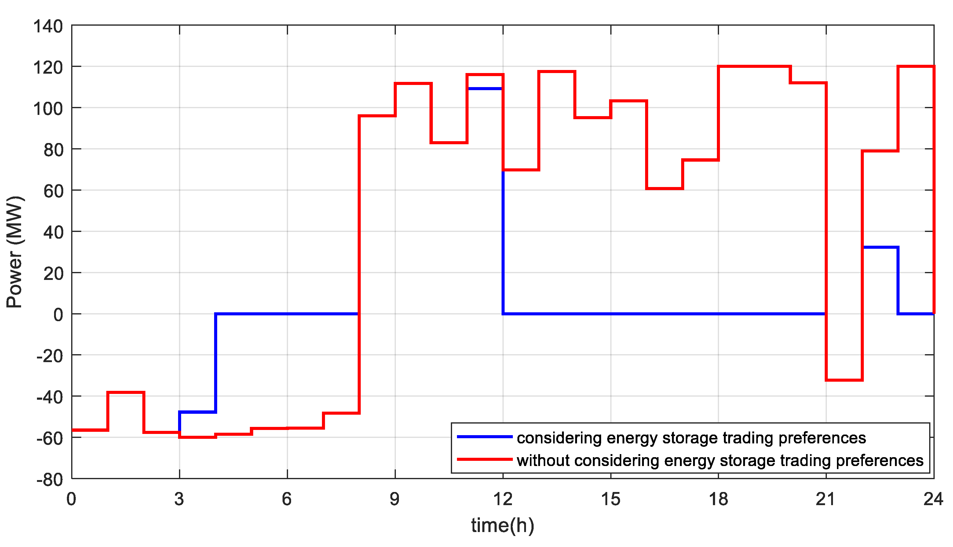
Figure 3 gives the variation in the charging and discharging power as well as the SOC value of the energy storage, considering the energy storage trading preference and without considering the energy storage trading preference. From the figure, it can be seen that the discharging power of energy storage increases significantly from 12:00 to 21:00 when energy storage trading preference is taken into account, which is due to the addition of charging and discharging time preference weights in the objective function of the trading model, guiding the deep discharging of the energy storage during the peak load time to alleviate the system congestion and to enhance the stability and reliability of the power system.

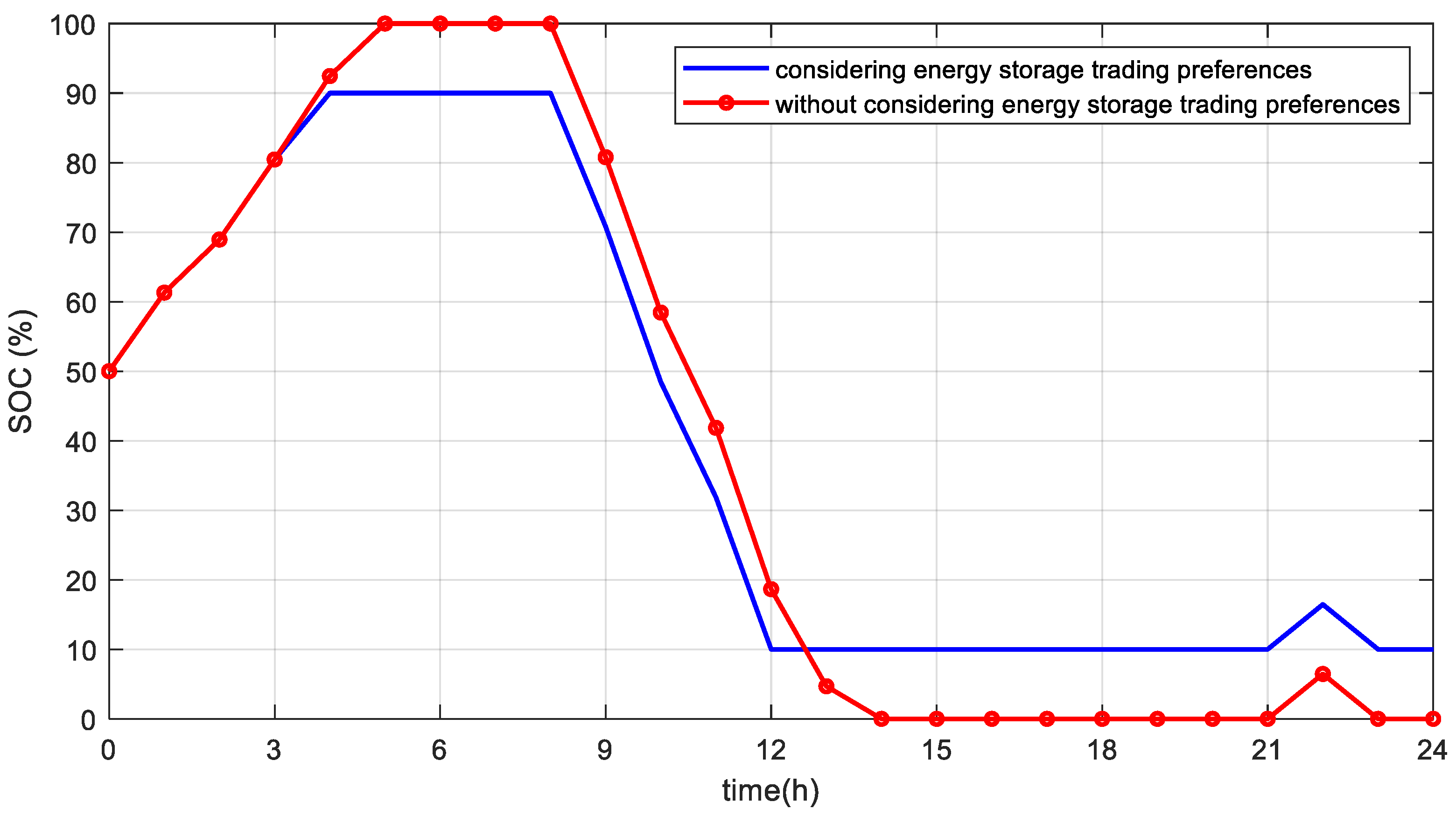
Figure 4 gives the change in SOC of energy storage under consideration of trading preference and without trading preference, from which it can be seen that energy storage still retains a 10% discharge margin at peak load when taking into account the trading preference of energy storage. This is because, under the effect of the risk factor, energy storage prefers to leave a certain amount of spare capacity to ensure that it can be used as a back-up power source to supply power to the system briefly to ensure the stable operation of the system in case of emergency and to avoid risks to the system due to overcharging or overdischarging.

Table 1. Clearing results under different time weight coefficients.

τdis	Percentage of Peak Discharges	Average Clearing Price (USD/MWh)	Systematic Peak-to-Valley Spread (USD/MWh)
1.0	68%	33.57	12.14
1.5	82%	32.57	10.29
2.0	91%	31.43	9.00

gives the clearing situation of energy storage participation in market trading under different time coefficients, and it can be seen from the figure that with the continuous improvement of energy storage in the peak load time, discharge accounts for more and more, the time preference coefficient did not increase by 0.5, and the peak discharge accounted for about 12%. At the same time, the system’s peak-valley spread will continue to decrease, which is due to the time preference of energy storage discharge leading to the concentration of energy storage in the peak load time discharges and thus depressing the system offer.

Table 2. Comparison at different life decay indexes.

γk	Average Number of Cycles (Cycles/Day)	Marginal Returns (USD/Day)
0	3.4	15.22
1.5	1.72	17.55
1.8	1.67	17.46
2.0	1.62	17.42

gives the values of the average number of cycles and marginal returns of the energy storage with different life decay coefficients. It can be seen from the table that the average number of cycles and the marginal gain of energy storage decrease with the increase in the lifetime decay factor, but, in general, they tend to be stabilized. Compared with ${\gamma }_k$ = 0 (without considering the life decay), the preference modeling can reduce the number of cycles of the energy storage, indirectly increase the life of the energy storage and increase the marginal return.

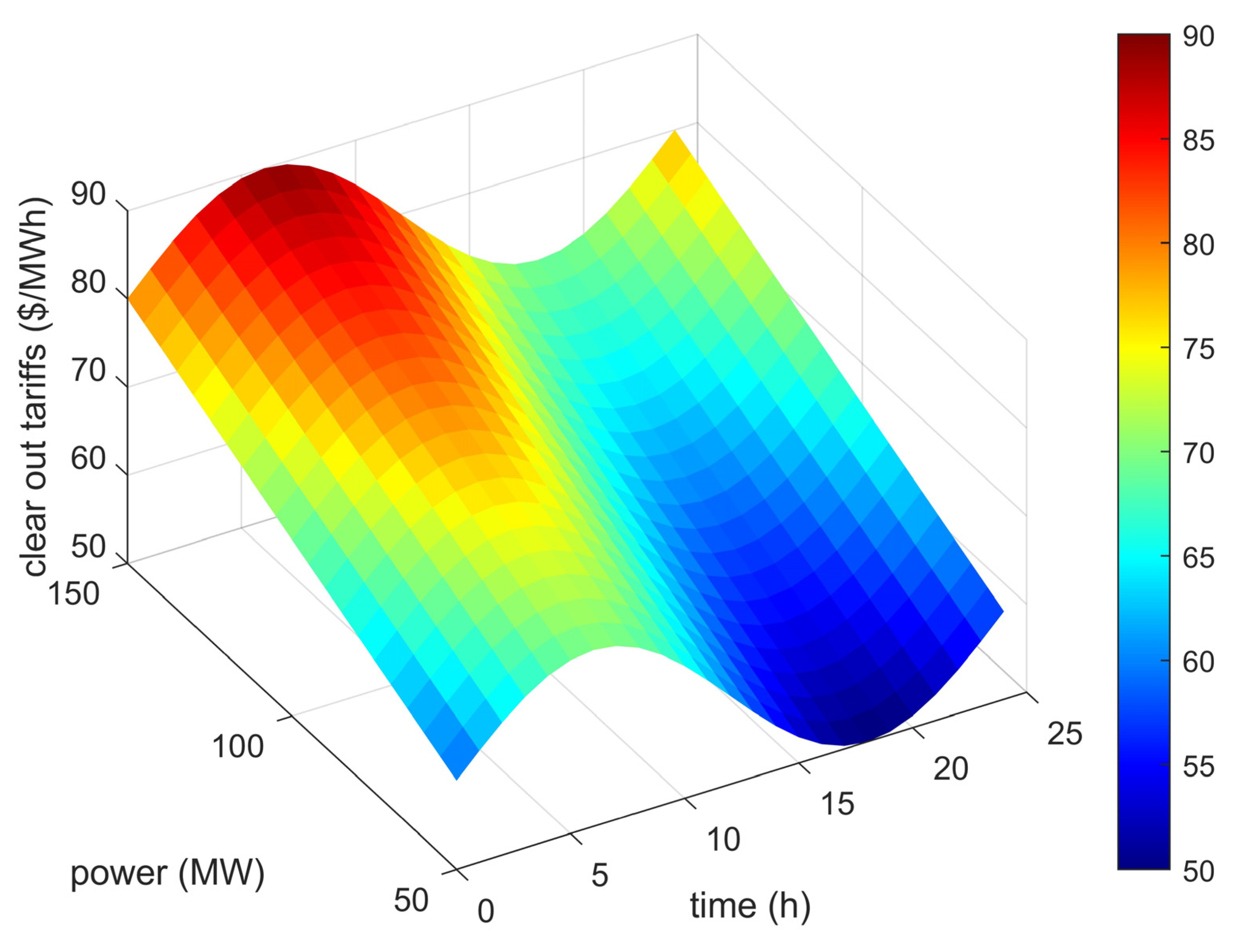
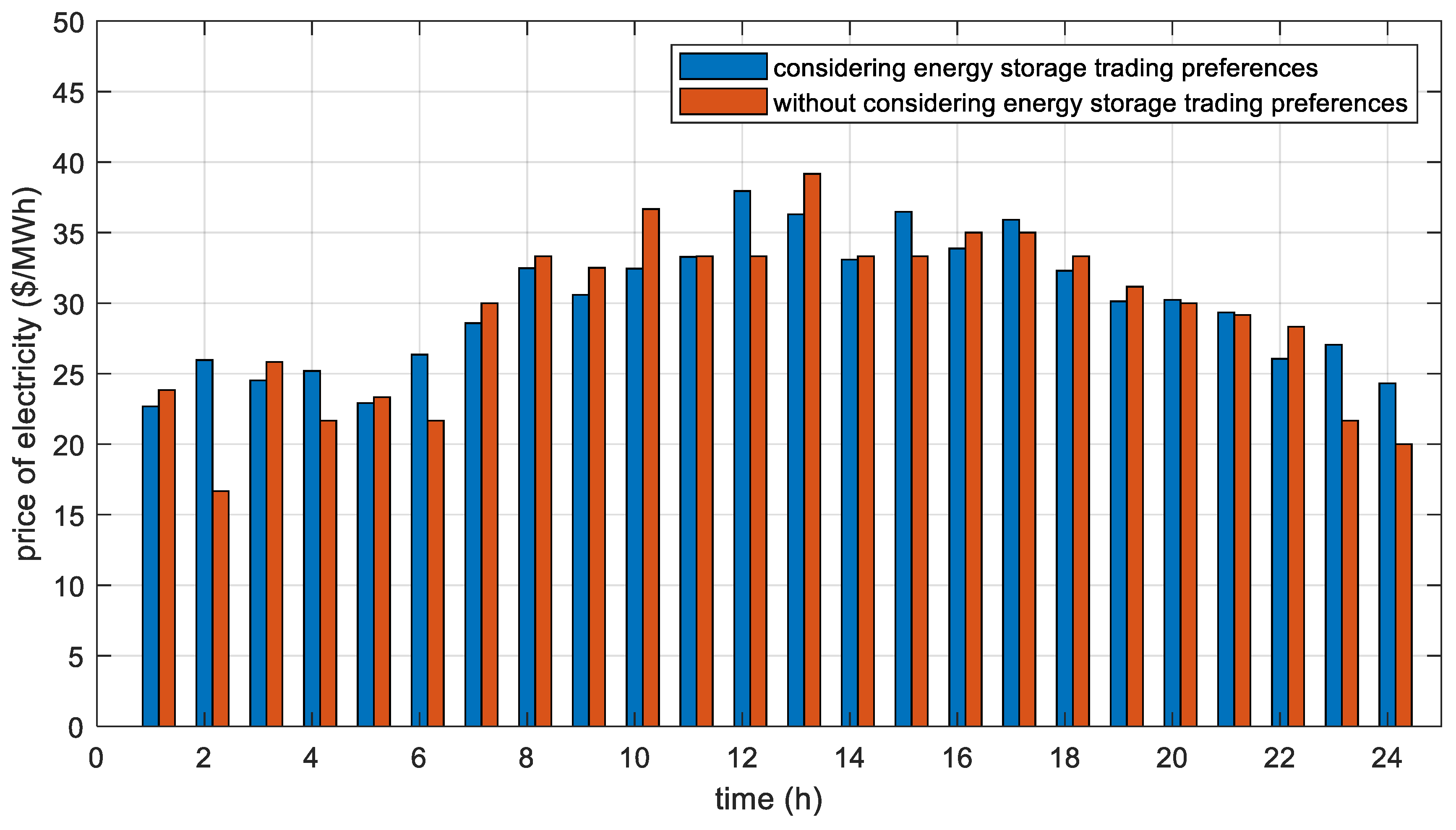
Figure 5 gives the clearing tariffs for storage participation in the spot market at different load levels. The comparison curve of the clearing price of energy storage with and without trading preference is given in Figure 6, from which it can be seen that the fluctuation amplitude of the system clearing price is significantly reduced after the introduction of the trading preference model. During peak load hours (e.g., 12:00–14:00), the clearing price is lower than that of the traditional model by 2.14–2.57 USD/MWh, while the price is higher by about 0.71–1.14 USD/MWh during low load hours (e.g., 03:00–05:00), which is essentially the result of the strategic charging and discharging behaviors of the storage operators under the framework of the trading preference that restructures the market supply–demand relationship, reducing the imbalance between the market demand and supply, and thus making the clearing price more favorable to the system of the market, thus smoothing out the clearing price.

4.2. Numerical Analysis in Multiple Scenarios

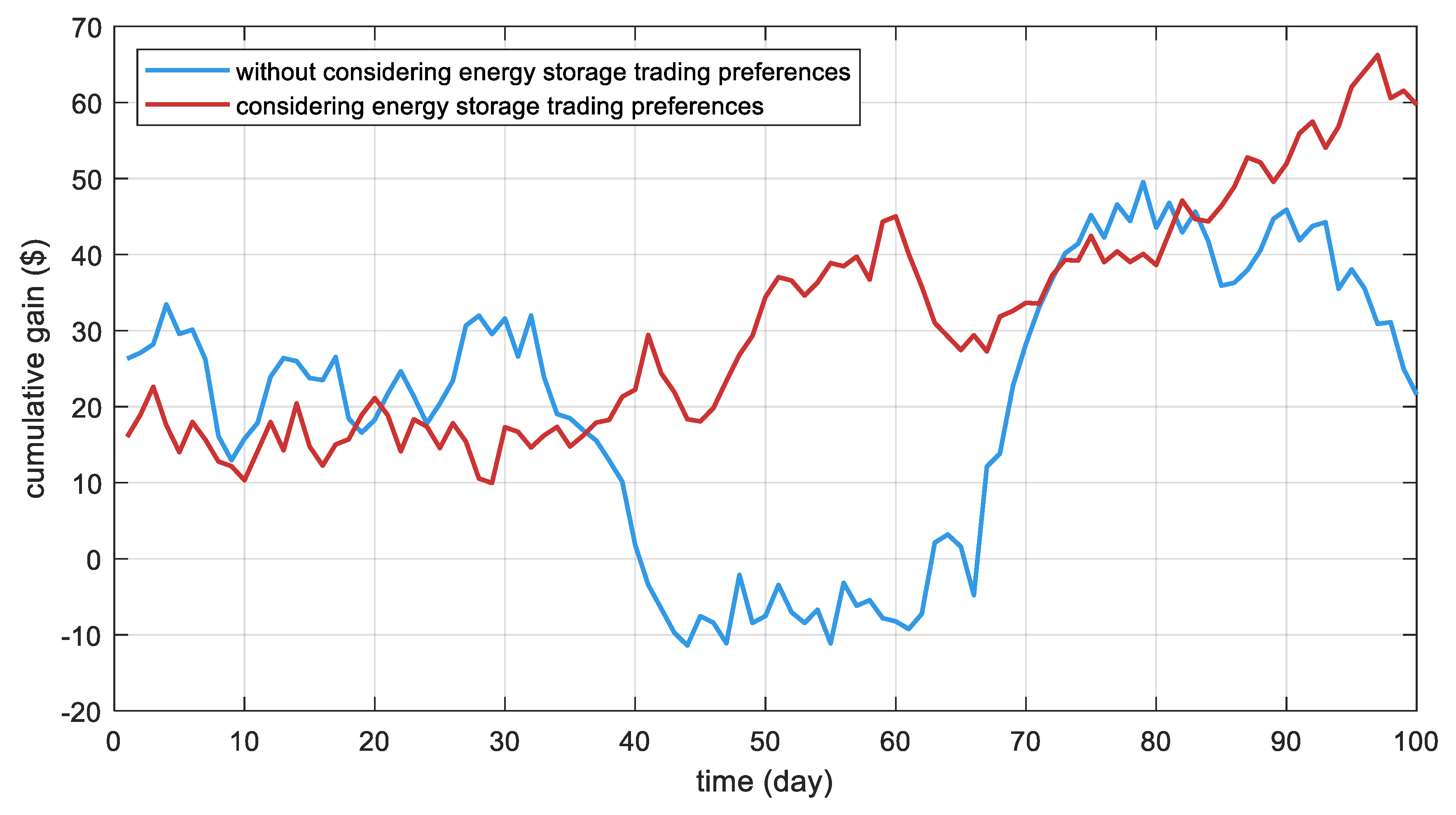
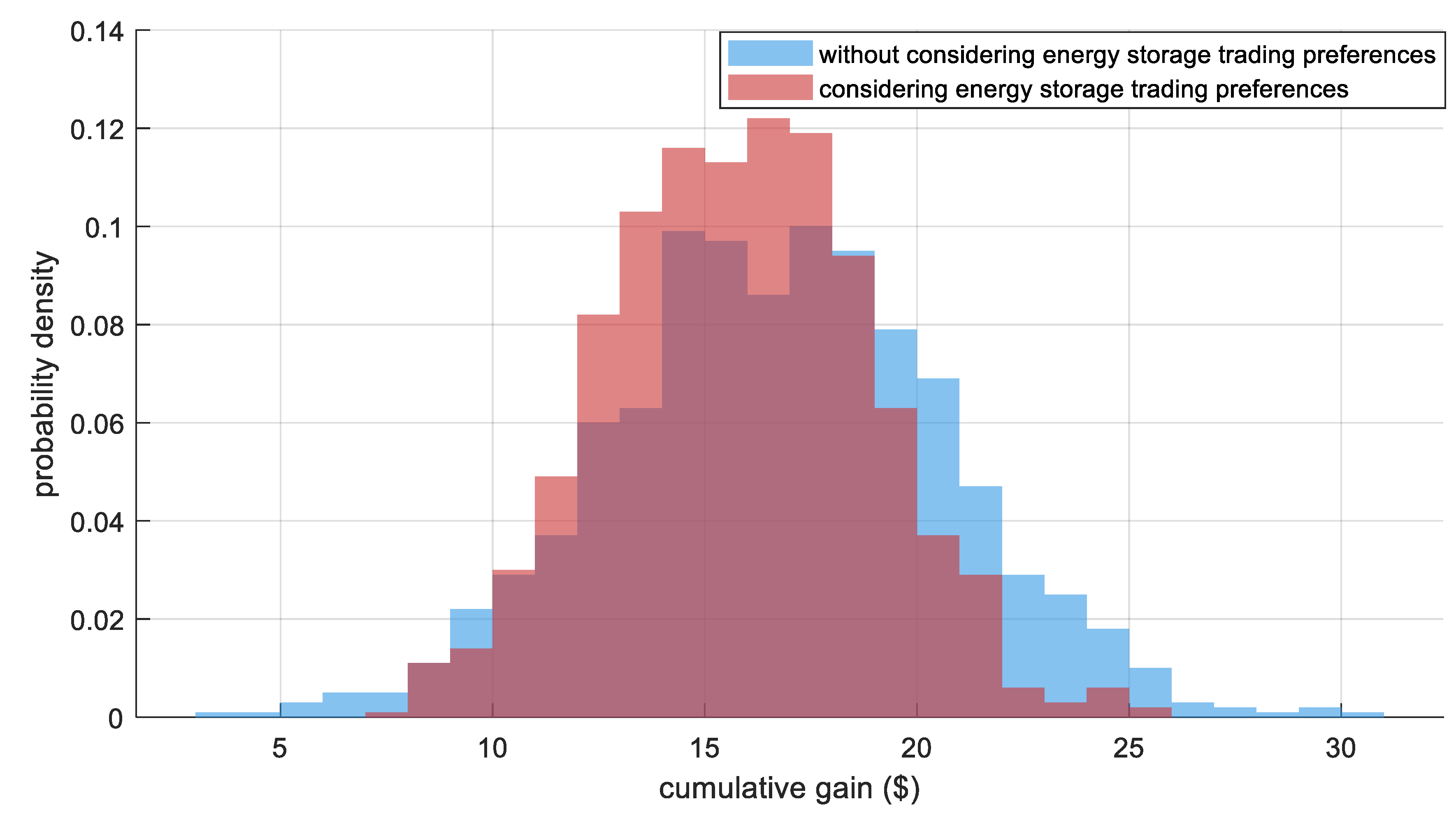
Figure 7 and Figure 8 give the cumulative returns with their probability distributions under the counting and storage trading preferences and the no storage trading preferences, respectively. From the figures, it can be seen that the cumulative returns of energy storage under the counting and storage trading preference are higher than those under the disregarding preference, and most of the returns of energy storage under the counting and storage preference come from peak tariffs, which is because the energy storage is more sensitive to the high-price period of the market under the high-risk preference and is more willing to trade when the price is higher. This strategy will lead to a higher overall return and a more concentrated probability distribution, which realizes the concentration and high level of return, thus improving its return efficiency in a limited time.

According to Figure 8, it can be seen that the return distribution of energy storage under the traditional trading model without considering the trading preference of energy storage shows a left-skewed pattern (skewness = −0.37), and its 10% quantile return is USD 12.14, which is significantly lower than the mean value (USD 17.71), indicating that there is a higher tail risk under the fluctuation of electricity price. In contrast, the model in this paper, by introducing CVaR control, has a return distribution that is right-skewed (skewness = 0.23), and the 10% quantile return is enhanced to USD 18.71, and the right tail extends to USD 22.57, which verifies its suppression effect on extreme losses. Further analysis reveals that the maximum retraction under the electricity price plunge scenario (the latter 5% quantile) is USD 26.43, which is 38.7% lower compared to that under no preference, highlighting the moderating effect of the risk preference parameter beta.

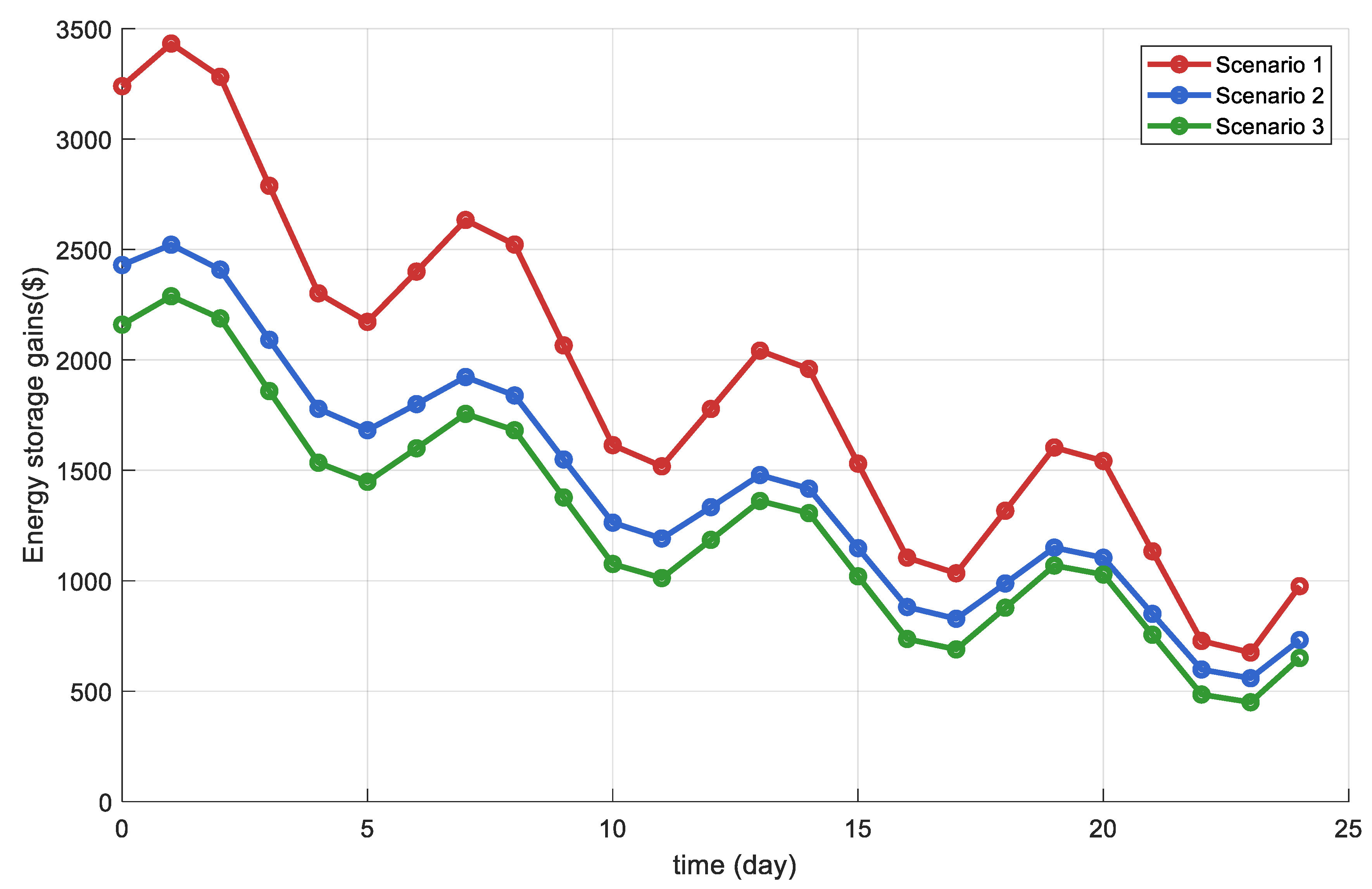
In order to analyze the impact of different trading preferences on the revenue of energy storage operators, this paper sets up the following three scenarios for comparison:

Scenario 1: Consider only tariff arbitrage gains (traditional single-tier model, ignoring cycling losses and risk appetite);

Scenario 2: Introducing circulating loss cost but no risk control;

Scenario 3: the model in this paper (combined tariff return, circulating loss cost and CVaR risk control).

From

Table 3. Comparison of benefits in different scenarios.

	Scenario 1	Scenario 2	Scenario 3
Average daily income (USD)	1778.57	1568.57	1674.29
Average number of cycles per day	1.8	1.2	1.4
CvaR (confidence level 95%)	2850	2400	1950
SOC fluctuation range (%)	20–100	30–90	40–85

, it can be seen that Scenario 1 has the highest average daily gain (USD 1778.57) due to ignoring cycling loss and overdischarging during peak hours (SOC reduced to 20%), but the number of cycles reaches 1.8 times/day, and the equivalent lifetime is only about 9 years (based on 6000 cycles). Scenario 3 reduces the average number of cycles per day to 1.4 and extends the lifetime to 11.4 years by balancing the gain with the cycling loss, while increasing the gain (USD 1674.29) by 6.7% compared to Scenario 2. The introduction of the CVaR risk term in Scenario 3I results in a right-skewed distribution of returns (Figure 7), a 42% reduction in the maximum retraction under extreme loss scenarios (e.g., electricity price plunge), and a reduction in the CVaR value from USD 407.14 to USD 278.57 in Scenario 1, which validates the model’s effective management of tail risk. Influenced by the time preference weights, Scenario 3 has a 75% share of discharging power during the peak electricity price hours (14:00–18:00) and a 68% share of charging during the trough hours (00:00–06:00), which is in line with the preset time preference.

In order to verify the effectiveness of the model proposed in this paper under different fluctuating electricity prices, this paper sets up the following three scenarios for comparative analysis:

Scenario 1: extreme electricity price volatility (standard deviation of electricity price is 7.14 USD/MWh);

Scenario 2: high electricity price volatility (standard deviation of electricity price is 4.29 USD/MWh);

Scenario 3: low electricity price fluctuation (standard deviation of electricity price is 1.43 USD/MWh).

Figure 9 shows the benefits of energy storage participation in the spot market under multiple scenarios. When the level of electricity price volatility is relatively low, energy storage is less motivated to participate in the market due to its trading preferences, which results in a lower level of benefits. As the level of price volatility increases, the incentive for energy storage to participate in the market becomes higher, and the return increases accordingly, with the return of energy storage increasing by about 41% under extreme price volatility.

From

Table 4. Comparison of returns in different scenarios.

	Considering Trading Preferences	Without Considering Trading Preferences
scenario 1	USD 1989.8	USD 1655.2
scenario 2	USD 1496.7	USD 1265.7
scenario 3	USD 1365.2	USD 1243.2

, it can be seen that due to the increase in electricity price volatility, storage is more willing to gain revenue through the spread, while Scenario 1 has a revenue enhancement of about 20.23% (USD 1655.5 → USD 1989.2) after considering the trading preference. Scenario 2 and Scenario 3 have 18.2% and 9.8% revenue enhancement, respectively, after considering the trading preference, which indicates that the preference model makes energy storage have stable revenue enhancement under different levels of electricity price volatility, and the higher the level of electricity price volatility, the more obvious the enhancement effect is.

4.3. Numerical Analysis of the Actual Power Grid in a Region

In order to verify the universality of the two-layer model proposed in this paper, the simulation analysis is carried out with the actual data of a regional power grid as an example, and the system includes 51 units and 6 different types of energy storage with the following parameters shown in

Table 5. Parameters of the energy storage system.

Serial Number	Charge and Discharge Efficiency	Useful Life (Year)	Self-Discharge Rate	Response Speed
1	95%	20–25	1.5%	ms
2	70–80%	20–30	1%	ms
3	80–90%	30–40	0	ms
4	75–85%	30–50	0	min
5	40–65%	40–50	1%	min
6	85–90%	20–25	10%	ms

.

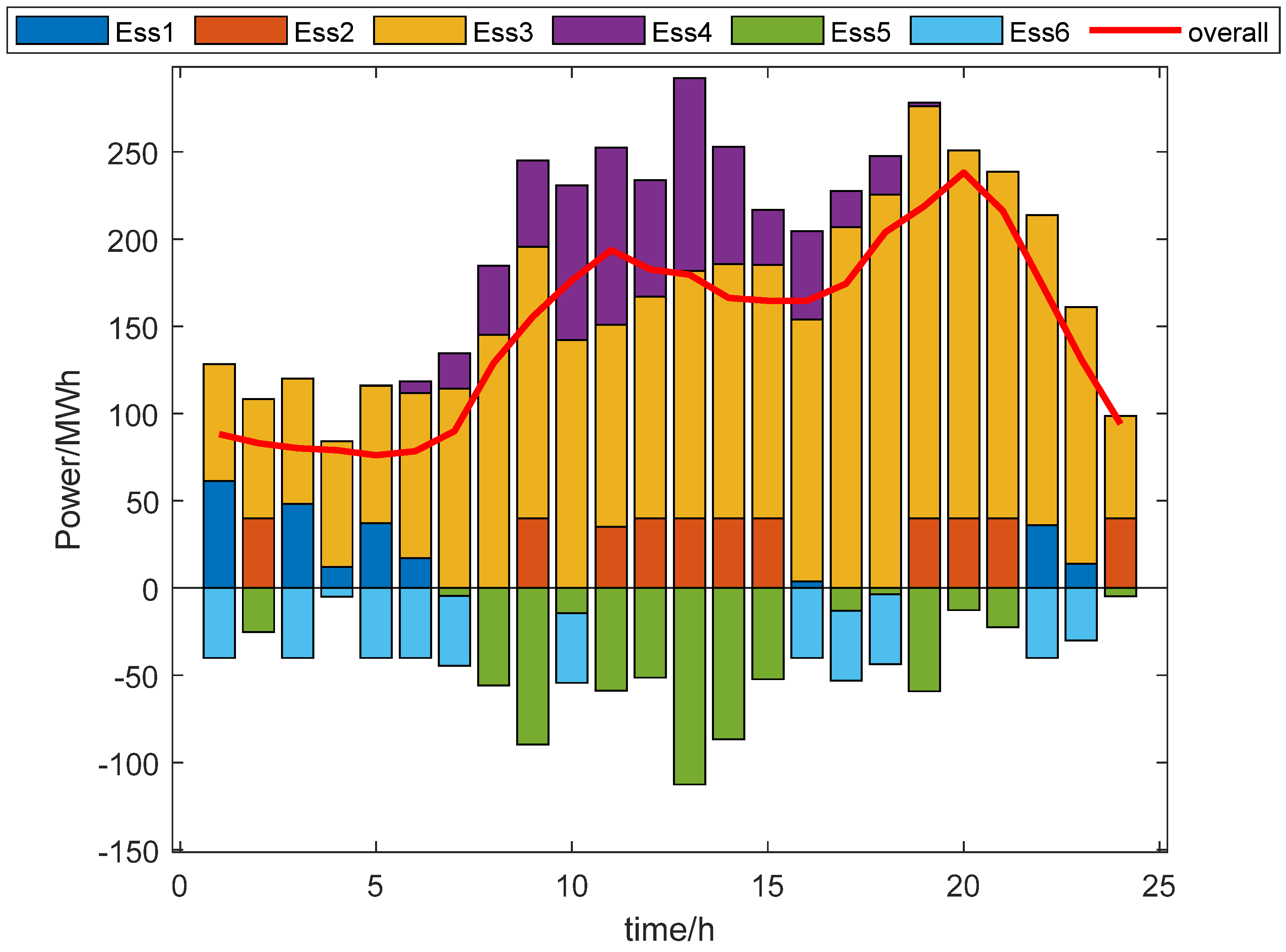
Figure 10 gives the energy storage participation in a regional spot market under the winning power of each storage. From the figure, it can be seen that different types of energy storage in the market have stable winning power, and in the peak load (16:00–20:00), when the total energy storage output is higher, in the load of the trough (0:00–4:00), when the total energy storage output is lower, the system, through the charging and discharging of energy storage, realizes the load transfer, and the system is beneficial to the economic and stable operation of the system. The system realizes load transfer by charging and discharging energy storage, which is conducive to the economic and stable operation of the system.

From

Table 6. Comparison with/without consideration of trading preferences.

	Considering Trading Preferences	Without Considering Trading Preferences
total system cost (USD/day)	17,530	19,752
average daily revenue from energy storage (USD/day)	7491	6324
average lifetime of energy storage (year)	30.37	28.26
energy storage revenue risk	38.7	49.6

, it can be seen that under the consideration of energy storage trading preference, the total system cost is reduced by about 11.2%, the average daily revenue of energy storage is improved by about 18.5%, the average life of energy storage is improved by about 7.5%, and the risk of energy storage revenue is reduced by about 21.9%. This shows that the two-layer model proposed in this paper can further improve the revenue of energy storage on the basis of guaranteeing the system operating cost, extending the operating life of energy storage and reducing the revenue risk, which is conducive to motivating the energy storage to participate in the market competition more actively and now balances the development of short-term arbitrage and long-term sustainability of energy storage.

5. Conclusions and Future Study

5.1. Conclusions

In this paper, we first propose a modeling method for energy storage trading preferences and establish charging time preference, price preference and risk preference models. The preference model is embedded into the trading model of the spot market through the weighting factor and utility function, and a provincial electricity spot market trading model taking into account the energy storage trading preference is proposed, and the model is solved through the KKT condition, and finally, the validity of the model is verified on an actual power grid in a region, and it can be seen through the analysis of the results that the proposed two-layer game model taking into account energy storage trading preferences shows significant multi-objective co-optimization ability in typical daily scenarios: compared with the traditional single-layer model, it reduces the equivalent number of cycles by 22.2% (1.8 → 1.4) and extends the battery life by 2.1 years (28.26 years → 30.37 years), while the average daily revenue is reduced by only 18.5% (USD 7491 → USD 6324), while the conditional value-at-risk (CVaR) is reduced by 7.5% (USD 49.6 → USD 38.7). This suggests that the model achieves an effective trade-off between short-term arbitrage gains and long-term sustainability by embedding cycle loss costs and CVaR risk control.

5.2. Future Study

This paper investigates a trading model that accounts for the trading preferences of energy storage and analyzes the trading preferences of energy storage from different dimensions, but there are still some problems that need to be solved, including the following:

(1)

The preference modeling process in this paper only considers the diversified trading preferences of energy storage participation in the electric energy market, and how to establish the trading preferences of energy storage participation in the future under the coupling of multilevel markets needs further research.

(2)

How to quantify the risk impact of multiple uncertainties (e.g., electricity price volatility, renewable energy output stochasticity) on decision-making [21] still needs to be deepened. In the future, we will construct a multi-stage stochastic planning model considering CVaR constraints to dynamically balance the energy storage operators’ returns and risk exposures through risk preference coefficients.

(3)

In existing studies, we focus on the design of market-based strategies for a single energy storage entity and have not yet fully explored the potential of smart buildings as flexible resource aggregators [22]. An in-depth discussion on the multidimensional trading preferences of shared energy storage and the modeling method of preferences under system uncertainty: this method can effectively solve the resource fragmentation problem of single storage operation while capturing the incentive role of market signals to the sharing economy model, which is conducive to the realization of a win-win situation between shared energy storage and the power grid.