Article

Application of Machine Learning Techniques for Predicting Heating Coil Performance in Building Heating Ventilation and Air Conditioning Systems

Department of Civil and Architectural Engineering and Construction Management, University of Cincinnati, Cincinnati, OH 45220, USA
*
Author to whom correspondence should be addressed.
Energies 2025, 18(9), 2314; https://doi.org/10.3390/en18092314
Submission received: 5 April 2025 / Revised: 25 April 2025 / Accepted: 27 April 2025 / Published: 30 April 2025
(This article belongs to the Special Issue Building Energy Performance Modelling and Simulation)

Abstract

:
Heating systems in a building’s mechanical infrastructure account for a significant share of global building energy consumption, underscoring the need for improved efficiency. This study evaluates 31 predictive models—including neural networks, gradient boosting (XGBoost), bagging, and multiple linear regression (MLR) as a baseline—to estimate heating-coil performance. Experiments were conducted on a water-based air-handling unit (AHU), and the dataset was cleaned to eliminate illogical and missing values before training and validation. Among the evaluated models, neural networks, gradient boosting, and bagging demonstrated superior accuracy across various error metrics. Bagging offered the best balance between outlier robustness and pattern recognition, while neural networks showed strong capability in capturing complex relationships. An input-importance analysis further identified key variables influencing model predictions. Future work should focus on refining these modeling techniques and expanding their application to other HVAC components to improve adaptability and efficiency.

1. Introduction

1.1. Issue at Large

Building occupants require a thermally comfortable environment to perform daily tasks efficiently and enhance overall productivity [1,2,3]. To achieve this, various HVAC systems are designed to regulate indoor temperatures based on occupant needs and external conditions. However, the energy consumption of these systems has significantly increased operational costs, making efficiency a critical concern [4].
Improving overall HVAC system efficiency requires a thorough evaluation of actual equipment performance under real-world operating conditions. A critical component of HVAC systems is the air handling unit (AHU), which conditions and distributes supply air through heating and cooling processes. The AHU consists of several key components, including heating and cooling coils, fans, air filters, and dampers, all of which contribute to indoor air quality and thermal comfort. The air filter removes particulates from the incoming air before conditioning, while the fan ensures proper air distribution through the ductwork. Figure 1 illustrates a typical AHU configuration with its major components. The heating coil is supplied with hot water from a gas-fired or electric boiler, whereas the cooling coil is connected to a chiller, cooling tower, or an air-source system, depending on the building’s design and climate conditions. These components play a crucial role in regulating indoor temperature and occupant comfort [5,6].
According to the U.S. Energy Information Administration (EIA), space heating accounts for the largest single energy end-use in commercial buildings, representing approximately 32% of total building energy consumption in the United States [7]. This high energy demand translates to substantial operational costs, particularly in colder climates, where heating loads are more significant. Additionally, the majority of heating energy is supplied by natural gas, a primary contributor to global CO2 emissions, highlighting the urgent need for energy-efficient heating solutions [8].
Heating coil plays a vital role in satisfying building’s heating load by transferring thermal energy from the hot water loop to the supply air. This process occurs as air is forced over the coil and distributed into occupied spaces, ensuring thermal comfort. The coil’s heat transfer characteristics significantly impact on the overall performance and efficiency of the HVAC system. Therefore, developing reliable and accurate energy models to predict heating coil performance is essential. Such models not only enhance system performance evaluation but also serve as a critical tool for optimization applications, improving energy efficiency and reducing operational costs [9].

1.2. Industry Trends

Modern HVAC research and industry trends emphasize decarbonization, electrification, and AI-driven optimization, increasing the demand for accurate heating coil models. The transition from fossil fuel-based heating systems to electric heat pumps and district heating networks necessitates precise performance modeling of heating components to maximize energy efficiency and minimize operational costs [10,11,12,13]. Furthermore, AI-driven optimization and digital twin technologies are being increasingly utilized to predict HVAC performance in real time, allowing for adaptive control strategies and improved fault detection [13,14,15]. Additionally, stringent energy codes such as ASHRAE 90.1 (American Society of Heating Refrigeration and Air-Conditioning Engineers) [16], international energy conversation codes [17], and global carbon reduction policies [18], are driving the need for more energy-efficient heating solutions, reinforcing the importance of accurate heating coil models. Current research has yet to establish a consistently reliable method for predicting HVAC system performance functions, in a way that directly enhances overall system efficiency. Developing new models will increase the likelihood of finding an optimal model to improve overall system efficiency.

2. Adoption of Data-Based Models to Predict Heating Coil Performance

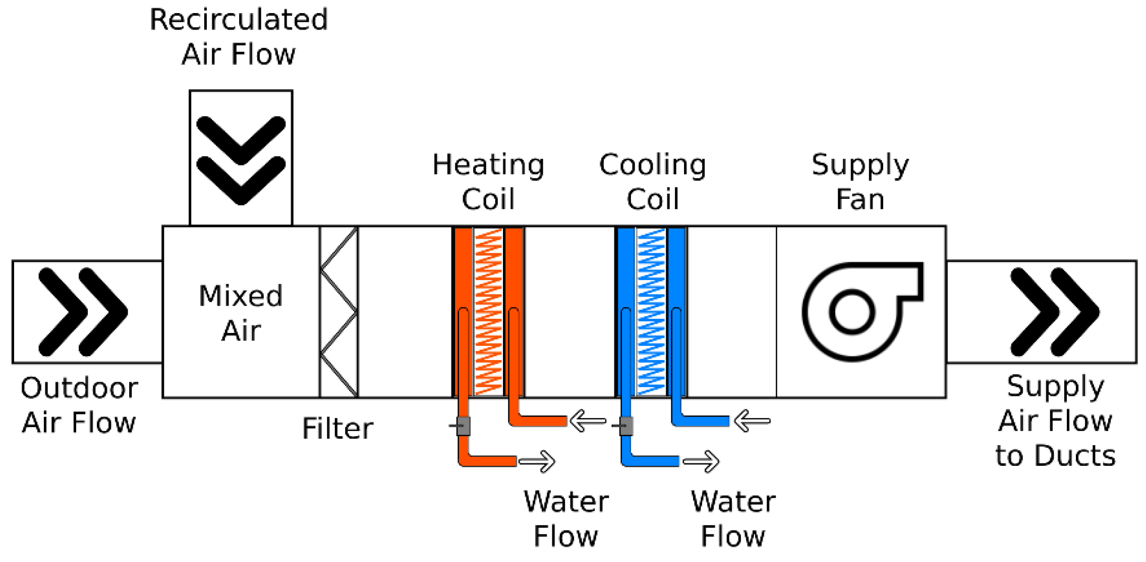
2.1. Performance Prediction of the Heating Coil

Despite the growing emphasis on HVAC efficiency, a review of past literature reveals that limited attention has been given to accurately predict heating coil performance using laboratory tested or real-world data. Early research by Barney and Florez focused on temperature prediction models for heating system control [19]. Asamoah and Shittu explored methods to predict heating and cooling loads in residential buildings using building energy models [20]. More recently, researchers have explored AI-based optimization for HVAC system operations [21] and machine learning techniques for air conditioning load prediction [22]. Although advanced data analysis methods such as deep learning for indoor temperature prediction [23], AI-assisted HVAC controls [24], thermal comfort, and energy efficiency improvements [25] are gaining traction, much of this work relies on simulation-based data rather than actual equipment-tested data [26].
One of the key challenges in accurately modeling heating coil performance is the lack of experimental datasets. Most research has focused on cooling coil loads [27,28,29], damper controls [30], thermal comfort improvements [31], fault detection [15,32], HVAC control optimization [33], and broader energy efficiency measures [34], etc. However, heating loads are just as critical, yet research on heating coil performance remains limited due to data scarcity. The absence of comprehensive experimental datasets restricts the generalizability of data-driven models, making it difficult to develop reliable performance predictions [35]. Additionally, the thermal response of heating coils is highly dependent on airflow rates, water temperature fluctuations, and environmental conditions, which further complicates the development of static models capable of capturing actual performance [36].
Given the significant role of heating coils in building energy consumption, developing accurate and adaptable models is crucial for optimizing HVAC system efficiency. The key motivation for developing accurate heating coil performance models lies in their practical applications. Such models can enhance performance prediction under varying operating conditions, optimize energy efficiency to reduce operational costs, detect HVAC system faults to prevent failures, and provide real-time feedback when integrated with building automation systems (BAS). This, in turn, enables adaptive control strategies that improve overall system reliability and efficiency [16,37].
In the context of developing advanced data analysis models, it is essential to examine the data analysis methods commonly used in the industry. Understanding these established techniques provides a foundation for selecting and refining models that best suit the specific application.

2.2. Multiple Linear Regression Models (MLR)

Multiple linear regression (MLR) is the most straightforward and widely used method for predictive modelling, particularly suited for datasets with simple relationships [38]. MLR operates by formulating a simple equation that predicts a single output based on multiple input variables. By adjusting one input while holding the rest constant, the model estimates the impact of each variable on the output. The coefficients in the equation quantify these effects, with larger coefficients indicating a stronger influence on the predicted outcome. MLR remains interpretable and computationally efficient, making it a practical choice to prepare straightforward models for various applications. The following equation shows the general format of MLR.
y = x1b1 + x2b2 + … + xnbn
Here, y is the dependent variable; a is the output intercept; b1, b2, … bn are the coefficients; and x1, x2, … xn are independent variables also known as the known parameters.
The primary limitation of MLR arises from the assumptions it imposes on data. It assumes a linear relationship between variables, independence among inputs and normally distributed errors with constant variances [39,40]. If these conditions are met, MLR offers a simple yet effective model for accurate predictions. However, if these assumptions are violated, model predictions become unreliable, potentially leading to significant errors in analysis [41].

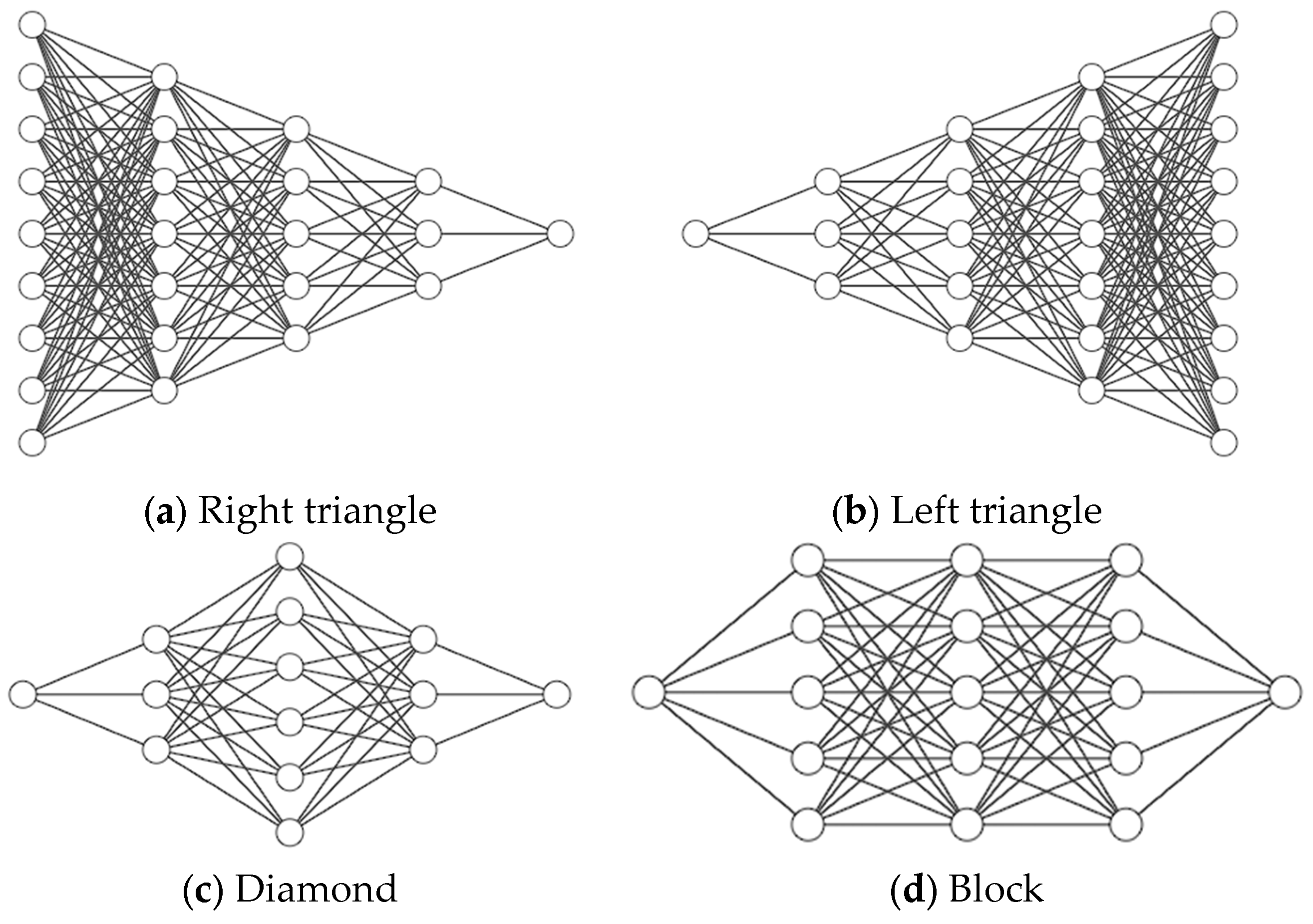
2.3. Neural Networks

Neural networks are a powerful method for simulating decision-making processes based on data inputs. They work particularly well, compared to other models, at recognizing complex patterns with multiple inputs and outputs. Neural networks often outperform simpler models that struggle to capture such relationships [42].
At its core, neural networks consist of multiple layers of interconnected nodes, that process and transmit information. These layers contain a predefined number of nodes, where each node represents a specific aspect of the data. These nodes perform computations based on an associated equation that applies weights to the inputs received from the previous layer. Structurally, this computation may resemble an MLR equation. However, in this case, the intercept is replaced by a bias term, which adjusts the activation threshold and coefficients, function as weights that regulate the influence of preceding node outputs, and the independent variables correspond to the values received from the previous layer.
Each node processes its inputs using an activation function, such as the hyperbolic tangent or sigmoid function, which determines how the output passes through to the subsequent nodes. These functions generate a value that controls the significance of a node’s contribution to the next layer. Figure 2 visualizes a selection of these activation functions, although there are many more variations exist, each with distinct properties suited for different modeling applications. A specific one to look at is the rectified linear unit or ReLU function, max(0, x), which gives a value of 0 to negative numbers and returns the exact same input for positive numbers.
Nodes in the subsequent layer interpret the activation function’s output value to determine the appropriate weight to assign on each node, or whether to consider it at all. The activation threshold is inversely related to the node’s importance; a lower activation threshold increases the node’s influence [43].
Neural networks refine their predictive capabilities by iteratively processing data and adjusting the weight of connections between nodes. This improvement occurs through a training process known as backpropagation, which propagates errors backwards from the output layer to the input layer. By analyzing the difference between predicted and actual values, backpropagation adjusts the connection weights to minimize the loss function, which quantifies prediction errors. A high loss value indicates significant deviation from the true value. The optimization process known as gradient descent iteratively adjusts the network parameters to move toward the closest minimum point of the loss function. Figure 3 shows how the calculated loss decreases over successive iterations, demonstrating the network’s improving accuracy [44].
During backpropagation, the network adjusts the weights of individual nodes based on predefined parameters. These parameters include bias calculations, learning rate, network architecture, iteration count, etc., contributing to the adaptability of neural networks [45]. Different network architectures such as right triangle (Figure 4a), left triangle (Figure 4b), diamond (Figure 4c), and block structures (Figure 4d) can significantly impact model performance. Architecture also relates to the number of nodes and layers, which influence the model’s capacity to learn complex patterns in data.
Increasing the number of nodes and layers enhances the network’s ability to capture intricate relationships but also raises the risk of overfitting, where the model memorizes training data instead of learning generalizable patterns. Overfit models perform exceptionally well on training data but fail to generalize unseen data. On the other hand, an insufficient number of nodes or layers may lead to underfitting, where the model oversimplifies patterns, reducing accuracy. Striking a balance between model complexity and generalization is crucial in neural network optimization, as it is across all machine learning paradigms. Given the vast number of possible configurations, optimizing a neural network often requires a combination of trial-and-error testing and advanced mathematical techniques [46]. By leveraging dynamic parameters and optimization techniques, neural networks provide a flexible and effective approach to pattern recognition, making them an essential tool in modern machine learning applications.

2.4. Bootstrap Aggregation (Bagging)

Bootstrap aggregation, also known as bagging, is a data modeling method that enhances predictive accuracy by training multiple models on randomly selected subsets of the data [47]. Bagging usually employs one of the following model types: decision trees, regressors, or classifiers. Individual instances of the selected models are trained on distinct subsets of the data. The aggregation of these models uses what is known as an ensemble technique. The ensemble ensures the final aggregated model is a proper accumulation of the individual models developed. Choice of the ensemble method must align with the base models used to ensure effective aggregation. Figure 5 highlights the process.
Generally, all models in the ensemble are typically assigned equal weight regardless of their individual performance. Consequently, bagging relies on the “wisdom of the crowd,” a belief that while any single model may not perfectly represent the entire dataset, combining multiple models leads to a more accurate and reliable prediction.
The performance of the model depends significantly on the number of models analyzed, which is directly correlated to the number of subsets. A larger number of subsets helps mitigate the influence of outliers but may narrow the data analysis of the models, increasing the risk of overfitting. A relatively lower number of subsets will generalize the data more but will be influenced by outliers. Consequently, the tuning of the sample size is essential to finding the optimal number of models [48].

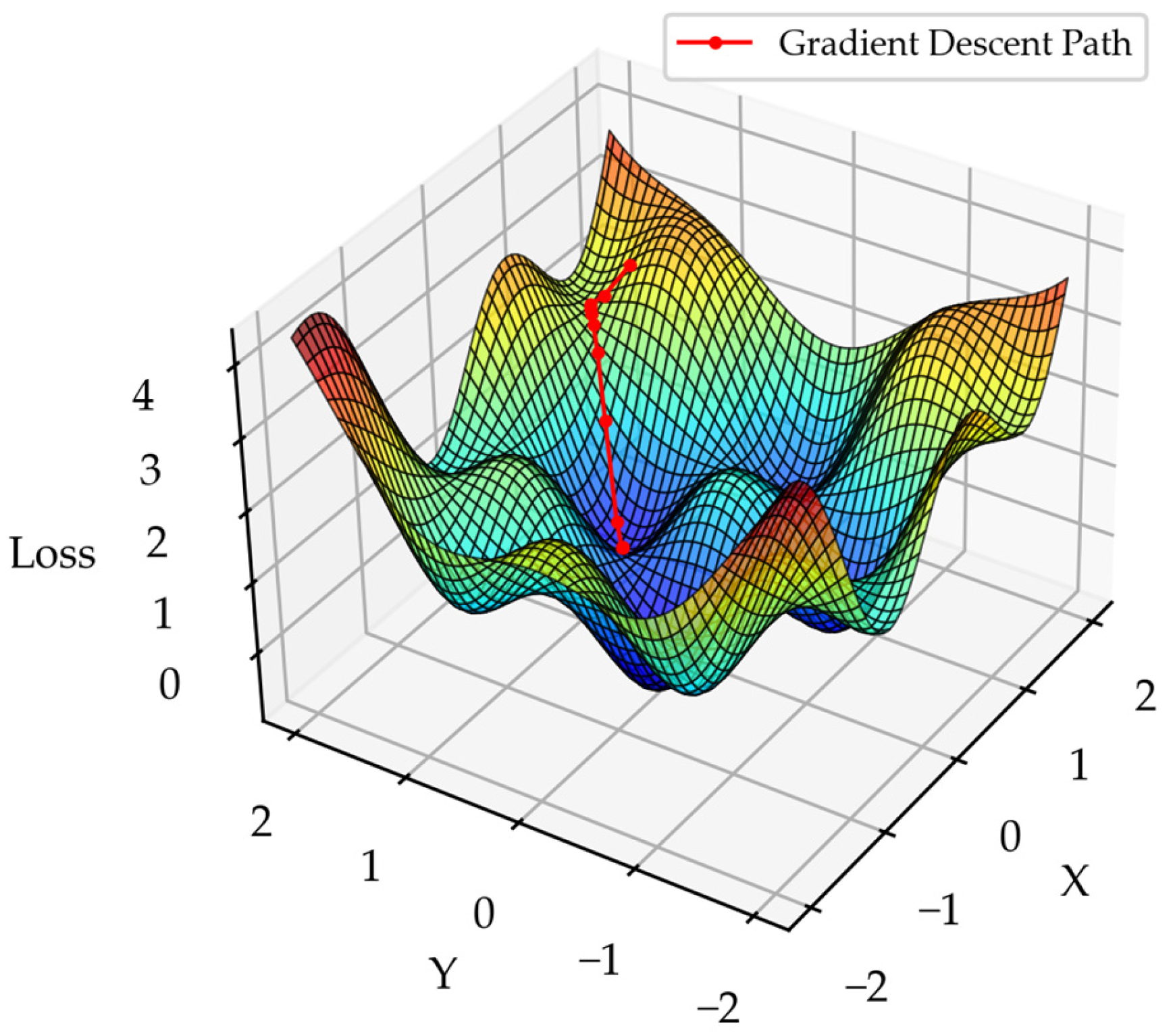
2.5. Gradient Boosting

Gradient boosting is another ensemble technique that improves predictive models through an iterative process whereby each model is trained independently to correct the errors of its predecessors [49]. Typically, decision trees are used as the base models, and each new model is added to the ensemble to enhance overall performance. The process is shown in Figure 6 below.
The first model developed is relatively simple, and each subsequent iteration refines it by focusing on residual errors to identify unrecognized patterns that the previous model failed to capture. Each addition to the ensemble is analyzed using a loss function, which determines the best adjustments needed to minimize prediction errors. This optimization process, known as gradient descent, aims to reduce the loss function. A loss function analyzes residual errors by comparing predicted and actual values, using techniques such as mean squared error to quantify discrepancies. Figure 7 shows a gradient descent path with two possible adjustment directions, labeled as x and y. While real-world models involve many possible adjustments, this figure conceptually represents how the algorithm identifies optimal modifications to reach a local minimum [50].
Each model in the ensemble finds its local minimum, and models with lower loss values are weighted more heavily, as they contribute more reliable predictions. This weighting is necessary because early models in the process tend to overgeneralize the data. Moreover, as the ensemble evolves, attempts to correct errors may lead to overfitting. By prioritizing models that minimize loss effectively, gradient boosting ensures that only the most accurate models contribute significantly to the final prediction [51]. While the fundamental principles of gradient boosting remain consistent, different adaptations prioritize various aspects, such as handling missing data or improving computational efficiency. Therefore, testing and fine-tuning different gradient-boosting variants are essential to achieve optimal performance.

2.6. Application of Advanced Data Analysis on Heating Coil Performance Prediction

This research aims to apply machine learning models, such as bagging, neural networks, and gradient boosting, to predict heating coil performance in building mechanical systems—specifically, to develop models that estimate supply air temperature based on the heating coil’s operation. Model selection is based on two key criteria: error analysis and model functionality. A chosen model must demonstrate acceptable predictive accuracy during both training and testing phases, with error thresholds determined by comparing the performance of all tested models. Since multiple models may meet these thresholds, it is also crucial to assess their underlying mechanisms and strengths.
In practical applications, dynamic models that effectively handle errors are essential. Given that HVAC systems operate with continuously changing data and require real-time decision-making, models must be capable of making logical adjustments based on all available information.

3. Methodology

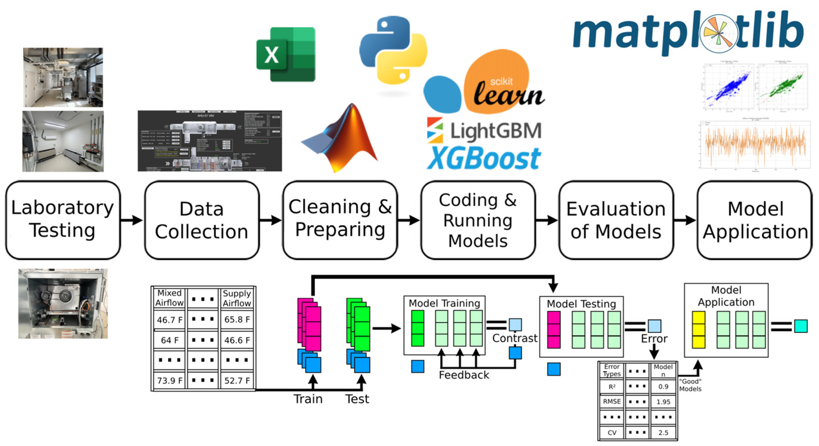
3.1. Overview of the Methodology

Figure 8 illustrates the overall workflow followed in this research. The process began with equipment testing to ensure compliance with basic standards and data accuracy. Once verified, data were collected in a large spreadsheet and cleaned to remove inconsistencies. The cleaned dataset was then formatted for implementation in the developed code. Next, various libraries, including matplotlib to create the figures, were utilized to train multiple machine learning models, which were evaluated based on their error metrics and predictive performance. Finally, the analysis focused on how these models could be applied in real-world scenarios. The figure also highlights key libraries and tools used at each stage of the process.

3.2. Laboratory Testing and Data Collection

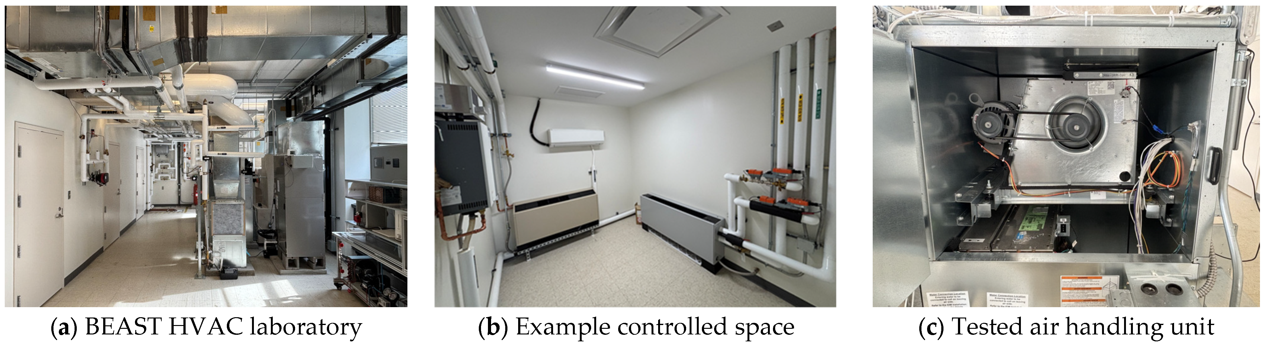
3.2.1. Overview of the Testing Facility

The experimental testing was conducted at the Building Energy Assessments, Solutions, and Technologies (BEAST) Laboratory (Figure 9a), located at the University of Cincinnati’s Victory Parkway campus. This facility is equipped with various HVAC systems, including variable refrigerant flow systems, water-based air handling units, and direct expansion units connected to an electric heater and an air-cooled chiller. Additionally, the lab features three well-insulated and controlled spaces (Figure 9b) designed to simulate actual building zones, each equipped with a variable air volume (VAV) box. For this study, testing was performed on a water-based air-handling unit (Figure 9c).
The laboratory’s centralized building automation system (BAS) was utilized to monitor and control equipment parameters, minimizing errors associated with manual adjustments.

3.2.2. Laboratory Testing Procedure

Laboratory testing of the heating coil was conducted during the winter season. Throughout the testing period, the cooling coil and chiller remained inactive, with all associated chilled water valves being fully closed. Testing spanned for one week, during which the laboratory’s BAS recorded system performance data at one-minute intervals, resulting in the collection of over 10,000 data points in imperial units.
To capture a broad range of operating conditions, the heating coil valve position and supply fan speeds were systematically adjusted every two hours. The heating coil valve position was incrementally modified from 20% (minimum valve position allowing at least 0.1 gallons per minute (GPM)) to 100% (maximum water flow) in 10% increments. A similar stepwise approach was applied to the supply fan speed, varying from 10% to 100% in 10% increments.
Precautions were taken to maintain the air handling unit’s internal temperature between 20 °F (−6.67 °C) and 95 °F (37.78 °C) to prevent freezing, which could affect the heating and cooling coils, and to avoid excessive heat buildup that could damage electrical switches and sensors. Additionally, all other HVAC components, including the cooling coil, VAV box heating coil, and humidifier, were deactivated to ensure they did not interfere with the air conditioning system. The three lab zones remained unoccupied and were not subjected to external influences throughout the testing period.
By adjusting the coil valve position incrementally, a comprehensive dataset was obtained covering a wide range of hot water flow conditions. The control signal modifications resulted in hot water flow variations ranging from 0.1 GPM (0.000006 m3/s) to a maximum of 1.6 GPM (0.0001 m3/s). While the valve position influenced the hot water flow rate, it did not alter the hot water supply temperature, which remained constant at approximately 120 °F (48.89 °C). The impact of supply fan speed variations on heating coil performance was also examined by assessing changes in supply air temperature under different airflow conditions. At 100% fan speed, the system achieved a maximum airflow of approximately 1300 cubic feet per minute (CFM) (2208.7 m3/h), representing the upper limit of the system’s capacity.
The testing covered a wide range of operating scenarios, from worst-case heating conditions to optimal performance cases. This approach ensured that extreme conditions were accounted for in the dataset, improving the robustness of the model predictions.

3.2.3. Hot Water Loop and Airflow Control Conditions

The air handling unit’s heating coil was supplied with hot water from an electric boiler connected through a closed-loop hot water system. The return water temperature varied based on system conditions. The supply air temperature was further influenced by outdoor and return air damper modulation, with the mixing air temperature maintained between 20 °F (−6.67 °C) and 95 °F (35 °C) to prevent freezing or overheating inside the unit.
During the testing period, outdoor temperatures dropped as low as −10 °F (−23.33 °C). It was ensured that no other conditioning sources influenced the supply air temperature besides the heating coil. The VAV damper positions remained fully open, and total supply airflow modulation was controlled solely by the supply fan.
This testing methodology enabled the collection of a diverse dataset that accurately represents real-world heating coil performance under various operational conditions, providing a strong foundation for predictive model development.

3.3. Basis of Developing Predictive Models and Data Cleaning

3.3.1. Data Cleaning

Following the completion of laboratory tests, key parameters influencing heating coil performance were identified. Initial results indicated that the supply air temperature conditioned through the heating coil was primarily influenced by the following variables:
  • Mixed air temperature (°F);
  • Supply water temperature of the heating coil (°F);
  • Hot water flow rate through the heating coil (GPM);
  • Total supply airflow (CFM).
Variations in these parameters directly impacted the supply air temperature. Based on this observation, the most influential factors determining heating coil performance were mixed air temperature, supply water temperature, hot water flow rate, and total supply airflow. Given this relationship, the supply air temperature was selected as the dependent variable, while the other identified parameters served as independent variables for model development.
Once the relevant parameters were finalized, data collected from the BAS underwent a structured cleaning process to ensure accuracy and reliability:
5.
Handling missing data: Any data entries with missing values, typically marked as “---”, were removed to prevent inconsistencies in the dataset.
6.
Eliminating transition period data: Since data collection was continuous, readings captured during input transition periods were excluded to ensure only stabilized values influenced the analysis. To do this, any fluctuations of 0.5 GPM (0.00003 m3/s) or greater in water flow and any fluctuations of 250 cfm (424.8 m3/h) or greater in airflow were removed.
In total, 260 data points were dropped. The cleaned dataset was then used to develop predictive models, with these models aiming to accurately represent the heating coil’s actual performance under varying operating conditions.

3.3.2. Development of Predictive Models

Predictive model development was conducted through Python 3.12.8 with the support of various libraries. Initially, MATLAB was considered due to its widespread use in engineering applications and its ability to produce visually appealing graphs. However, Python was ultimately chosen for its greater prevalence in machine learning applications, ease of use, and efficient computational capabilities. Python’s performance advantage lies in its ability to handle computationally intensive data analysis tasks by leveraging libraries that execute complex mathematical operations in C or C++ while maintaining user-friendly, readable code. With the help of selected libraries, which simplify intricate operations, the predictive models were successfully developed.

3.3.3. Splitting Data

To effectively train and evaluate the models, the dataset was divided into training and testing subsets. Typically, models perform well on training data but may struggle with unseen data during testing. The choice of data split ratio depends on the dataset size, with 80/20 and 70/30 being common practices. In this research, both split ratios yielded nearly identical results, indicating that the dataset was sufficient for model training. Consequently, a 70/30 split was used for figures and tables in this study. Additionally, a random state was set to ensure reproducibility in data partitioning. Since computers generate pseudo-random splits, the seed value determines the starting point for randomness. Various random states were tested, all producing consistent results, as expected. For this research, a random state of 0 was used in all figures and tables.

3.3.4. Library Selection and Model Evaluation

A total of 31 machine learning models were developed and tested in this study, utilizing key libraries such as scikit-learn, XGBoost, LightGBM, Pandas, and NumPy [52]. Pandas and NumPy serve as foundational libraries that support data processing and mathematical operations. Pandas facilitates data manipulation, handling structured data such as tables and time series [53], while NumPy provides Python with capabilities for vectorized computations, indexing, and managing large, multidimensional arrays and matrices [54]. These libraries, in combination with various machine learning frameworks, allowed for the implementation and fine-tuning of predictive models.
The primary objective of this study was to identify the most effective approach for predicting supply air temperature in a HVAC system. Given the variability of environmental conditions such as climate, humidity, and seasonal fluctuations, a single predictive formula would be insufficient. Therefore, models were evaluated based on performance metrics, adaptability, and suitability for real-world applications.
When multiple models demonstrated comparable predictive accuracy, a more detailed analysis was conducted to assess their individual strengths and limitations. The goal was to develop a robust and adaptive set of models capable of recognizing localized patterns and learning system-specific behaviors.

3.4. Error Metrics Calculation

Equation (2) through (6) define the error metrics used to assess model performance. While multiple error methods were analyzed, R2 (coefficient of determination) is the primary metric presented in most figures, as it measures how well the model’s predictions align with actual values. An R2 value of 1 indicates a perfect fit, while values below 0 suggest that the model performs worse than the mean value.
Mean absolute error (MAE) calculates the average absolute difference between predicted and actual values, treating all errors equally [55]. This method is effective when all data points hold equal importance. Mean squared error (MSE) determines the squared differences between predictions and actual values, penalizing larger errors more heavily [56]. This makes it useful when outliers significantly impact accuracy. Root mean squared error (RMSE) is similar to MSE but applies a square root to return the error to the original unit, making it easier to interpret. However, because RMSE applies a square root to the error, differences between models may appear less pronounced. For example, if one model has an MSE of 100 and another has an MSE of 81, the difference seems significant. But after applying the square root, their RMSE values become 10 and 9, making the difference appear smaller. Coefficient of variation (CV) evaluates whether a model is overfitting or excessively generalizing by analyzing its consistency across the dataset [2,57].
R 2 = 1 S u m   o f   S q u a r e s r e s i d u a l S u m   o f   S q u a r e s T o t a l
M A E = i = 1 N u m b e r   o f   O b s e r v a t i o n s O b s e r v e d   V a l u e s ( P r e d i c t e d   V a l u e s ) N u m b e r   o f   O b s e r v a t i o n s
M S E = i = 1 N u m b e r   o f   O b s e r v a t i o n s O b s e r v e d   V a l u e s ( P r e d i c t e d   V a l u e s ) 2 N u m b e r   o f   O b s e r v a t i o n s
R M S E = i = 1 N u m b e r   o f   O b s e r v a t i o n s O b s e r v e d   V a l u e s ( P r e d i c t e d   V a l u e s ) 2 N u m b e r   o f   O b s e r v a t i o n s
C V = 100 × R M S E O u t p u t M e a n

4. Results

4.1. Analysis of Models

Figure 10 compares the error values of all 31 tested models, providing an overview of their general performance. Refer Appendix A.1 for a better visualization of the R2 values. The results indicate that most approaches achieved similar accuracy in predicting supply air temperature. While a few underperformed, the majority produced strong predictions, suggesting that the dataset was not overly complex for selected algorithms.
Since different predictive techniques yielded comparable accuracy, selecting the best-performing ones requires more than just minimizing error values. Instead, additional practical considerations relevant to the field of study must be considered. For instance, when implemented in an actual system, predictive tools will inevitably encounter outliers, just as seen in the original dataset. Those capable of handling such anomalies effectively are preferred as they maintain performance stability during transitional periods when input conditions change. Another crucial aspect is adaptability. Given that not all HVAC systems are identical, models that can be adapted to different environments are more valuable. Based on these criteria, three models were selected: neural network, XGBoost, and bagging. Additionally, MLR was included as a baseline for comparison.

4.2. Model Selection

Four selected models offer strong potential for further development in machine learning applications. Neural networks, XGBoost, and Bagging demonstrated robust performance making them suitable for this research. However, it is reasonable to question why the voting regressor and random forest models, which achieved the lowest error values, were not selected. Several factors contributed to this decision.
While these models performed marginally better in terms of R2, their performance across other error metrics was either equivalent to or worse than the selected models. Additionally, when tested on uncleaned data, the bagging model outperformed both the voting regressor and random forest, as is shown in Figure 10, across the analyzed error metrics [58,59]. Table 1 represents the error values obtained without data cleaning.
Bagging and XGBoost, similar to neural networks, offer greater potential due to their ability to handle errors effectively and the availability of extensive tuning and adjustment options. Since all models performed well based on evaluated error indices, the selection prioritized models known for their reliability and adaptability in real-world applications.

4.3. Analysis and Discussion of the Selected Models
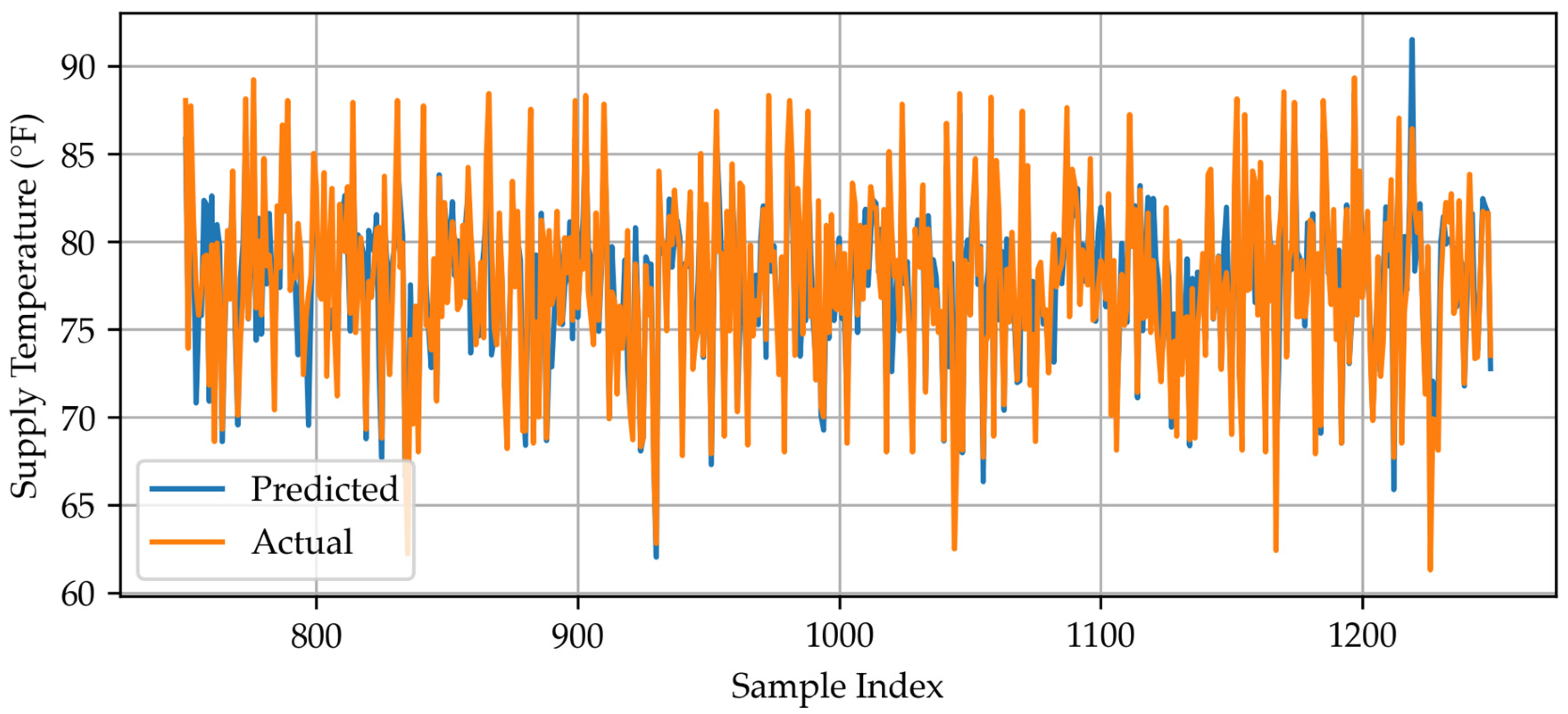
4.3.1. MLR

MLR was chosen as a baseline due to its simplicity and transparency. As a straightforward method, it provides a clear mathematical equation, making it useful for establishing benchmark error values and identifying key input variables that influence predictions. Comparing MLR’s insights with those from advanced models helps assess whether complex approaches capture the same underlying relationships or offer meaningful improvements beyond a linear framework. Given that many advanced techniques function as black boxes, MLR serves as a valuable reference for evaluating their effectiveness [60,61].
Equation (7) presents the developed MLR equation, illustrating how each input variable contributes to the predicted output. Among the independent variables, the mixed air temperature (x3) exerts the greatest influence, as indicated by its larger coefficient.
Y = 77.77 + 0.54 × x1 + 5.42 × x2 + 7.30 × x3 − 1.92 × x4
where y = supply air temperature (°F); x1 = hot water supply temperature (°F); x2 = water flow (gpm); x3 = mixed air temperature (°F); and x4 = supply fan air flow (cfm).
Figure 11 displays the testing and training scatter plots, along with residual plots, to analyze the accuracy of the model’s predictions. Figure 11a,b reveal that many data points deviate significantly from the ideal predicted values, forming noticeable clusters away from the regression line. Similarly, Appendix A.2 visualizes these discrepancies through a line plot. These observations suggest that while MLR effectively captures general trends, it struggles with accuracy and reliability, particularly when modeling intricate or nonlinear patterns in the data. The residual plots in Figure 11c,d further highlight this limitation, as a significant number of data points are far from the central regression line, demonstrating that MLR frequently fails to provide precise predictions.

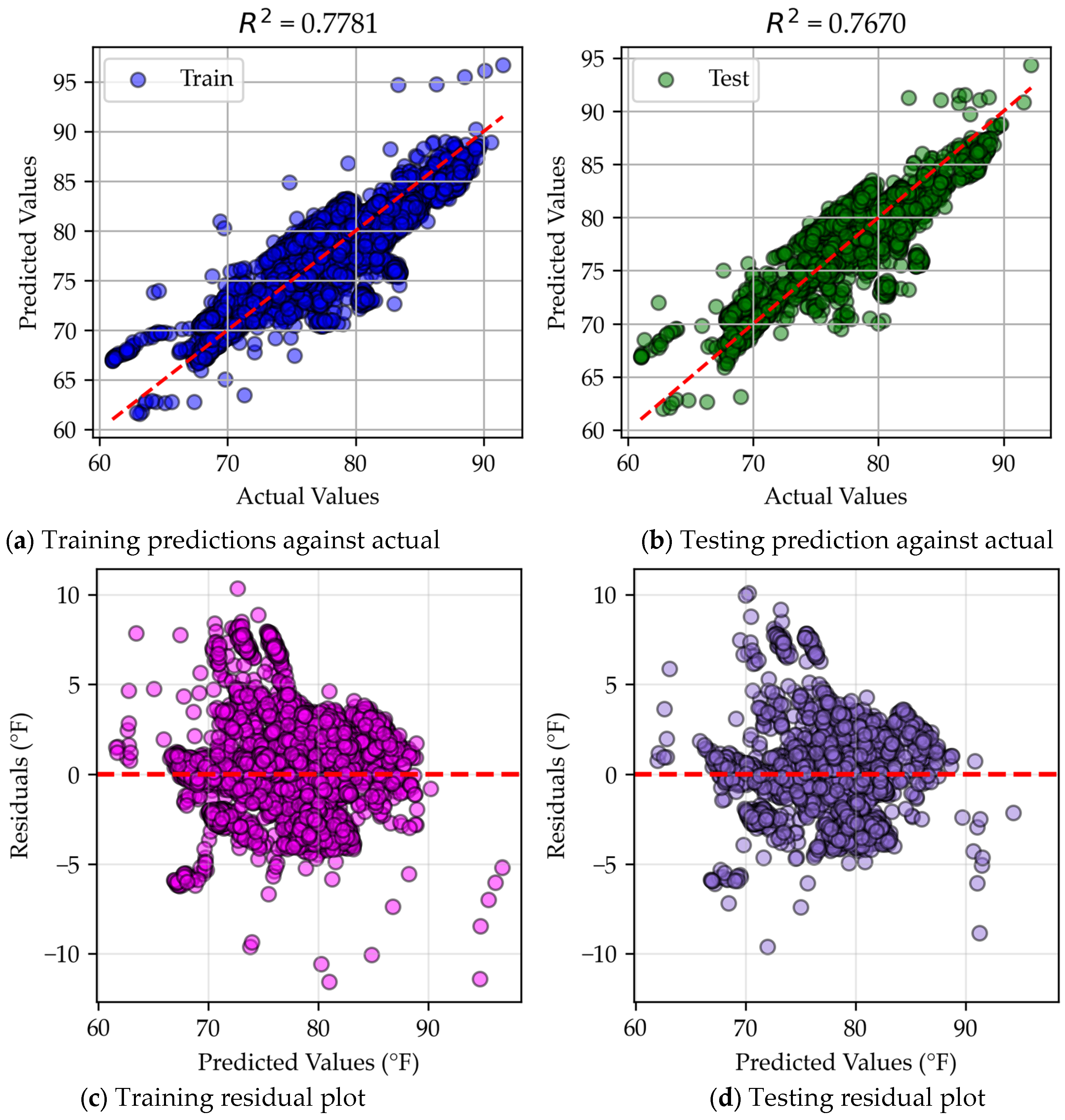
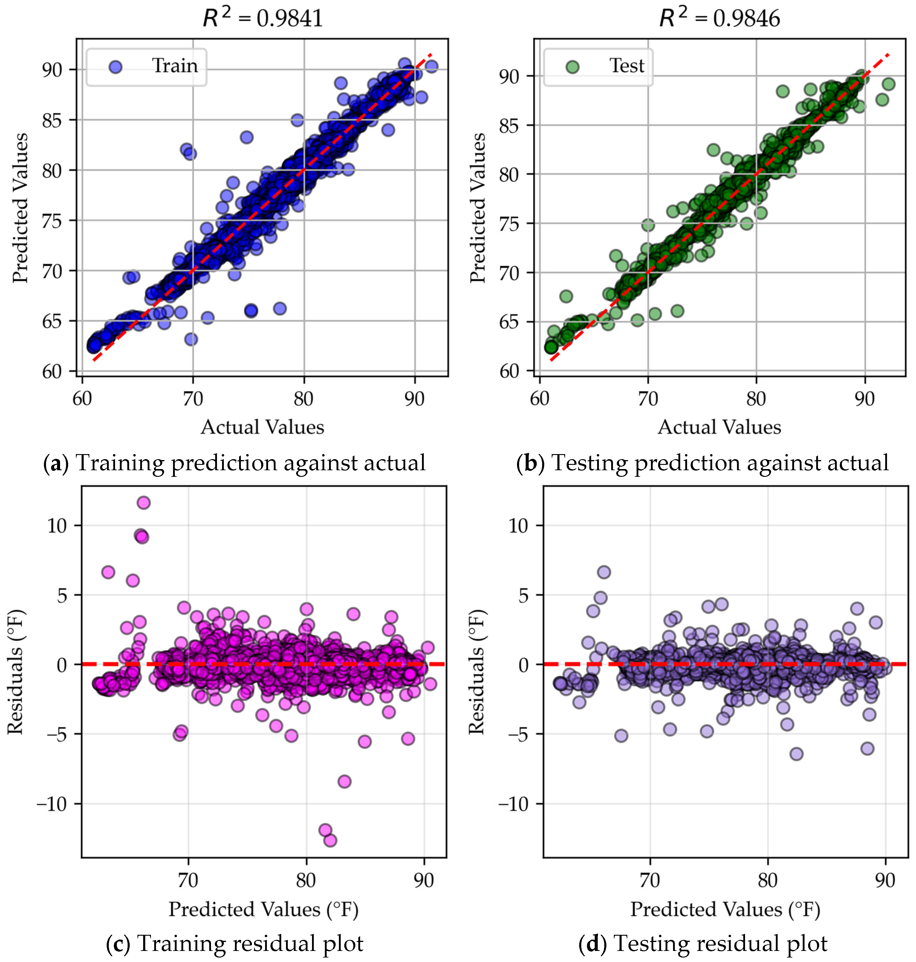
4.3.2. Neural Network

Neural networks were selected for their ability to model complex relationships with varying levels of complexity. The network architecture primarily consisted of single-layer or right-triangle configurations. Key parameters, such as the number of nodes and layers, were adjusted to identify an optimal predictive model, while bias calculation methods and learning rates remained constant [62]. Since larger networks require more iterations to fine-tune their weights effectively, structural modifications were necessary to balance accuracy and computational efficiency.
The best performing model in this study was a single layer neural network with 100 nodes using a ReLU activation function. While further refinements, such as adjusting the number of nodes or layers, could enhance accuracy, the model’s high performance made additional optimization unnecessary. Figure 12 illustrates a simplified neural network with only 10 nodes and their associated connection weights. Although this study may not have identified the most optimal neural network, the tested models demonstrated strong predictive capabilities. More advanced deep learning models could potentially outperform all tested configurations, but within the scope of this research, neural networks provided reliable predictions with some variability across different setups [63].
An analysis of the neural network residuals reveals an interesting trend in that its training and testing performance were nearly identical. By comparing Figure 13a,b, as well as Figure 13c,d, it was evident that the error values were consistent across both phases. Notably, the R2 value for the training dataset was slightly lower than that for the testing dataset, which appears counterintuitive at first glance. In other models, training typically outperforms testing, but this suggests that the neural network is operating near a local minimum. The model successfully identified patterns in the data and generalizes well to unseen inputs, but it has not necessarily reached a global minimum, as some other models marginally outperformed it. Even still, the neural network strikes a balance between generalization and overfitting. Nearly identical data distribution in both the training and testing scatterplots further supports this claim.
Unlike MLR, which relies on a generalized linear formula, neural networks can capture more complex patterns while maintaining consistency between training and testing results. Appendix A.3 presents an alternative visualization of residual data, reinforcing these observations.

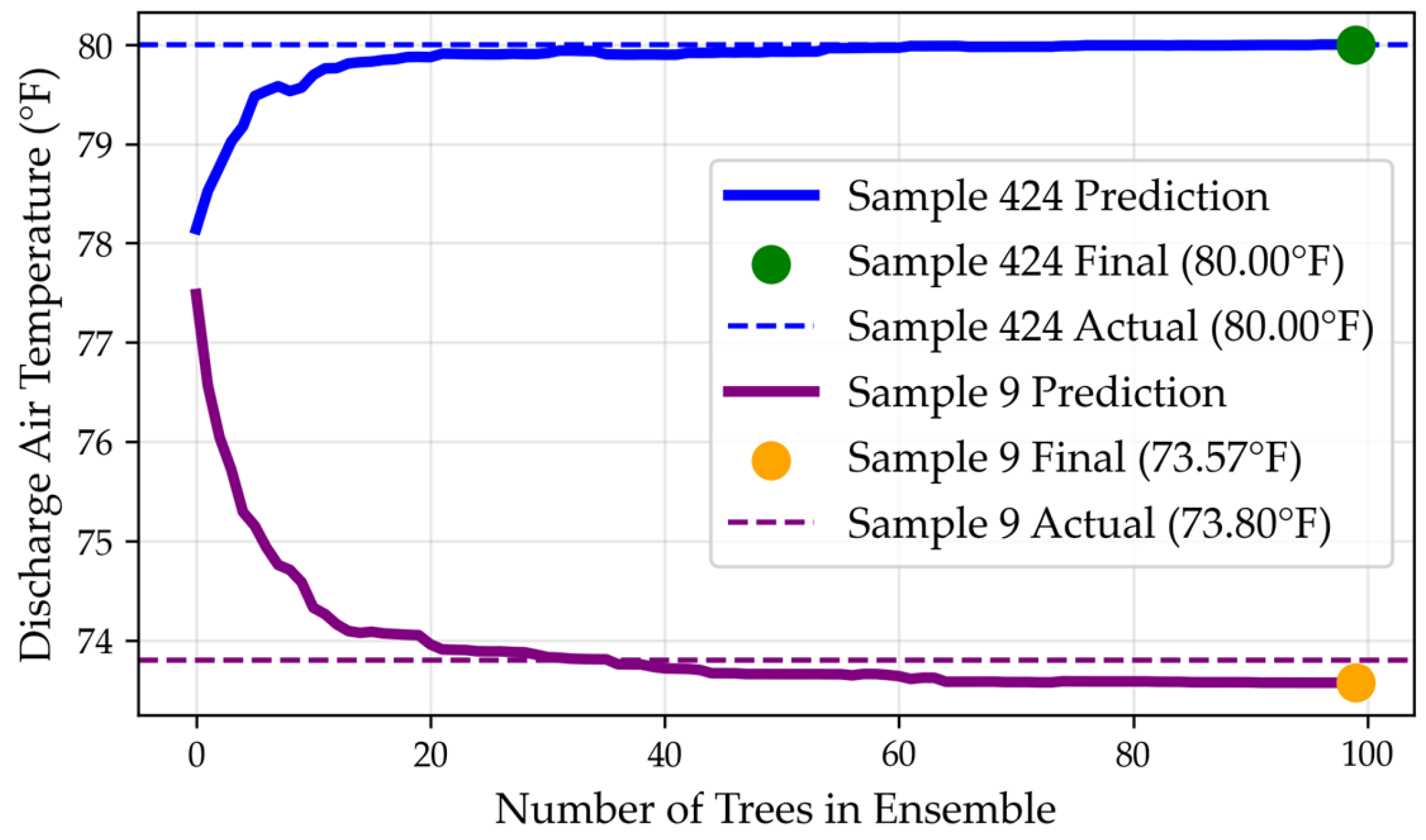
4.3.3. Gradient Boosting
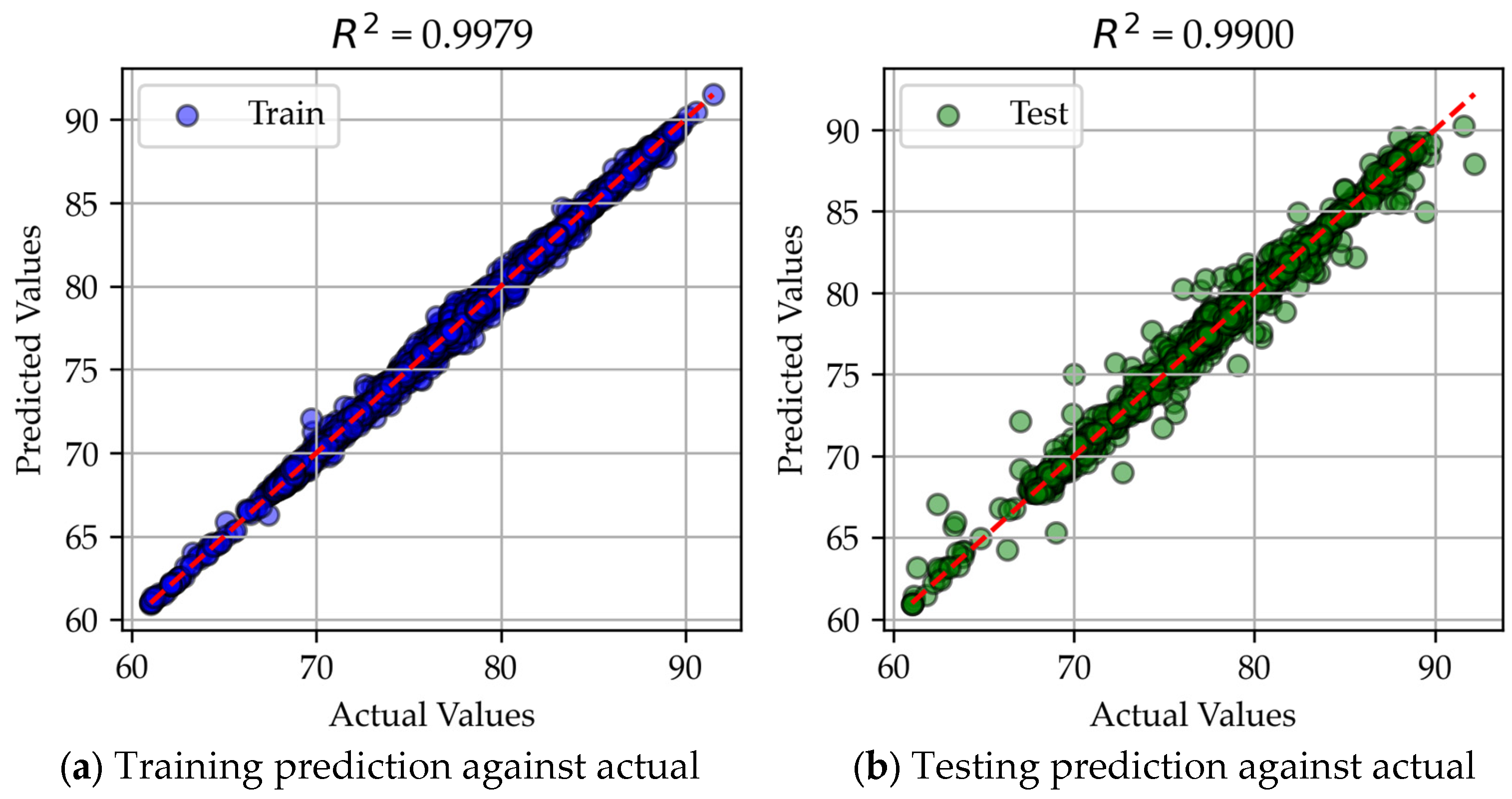
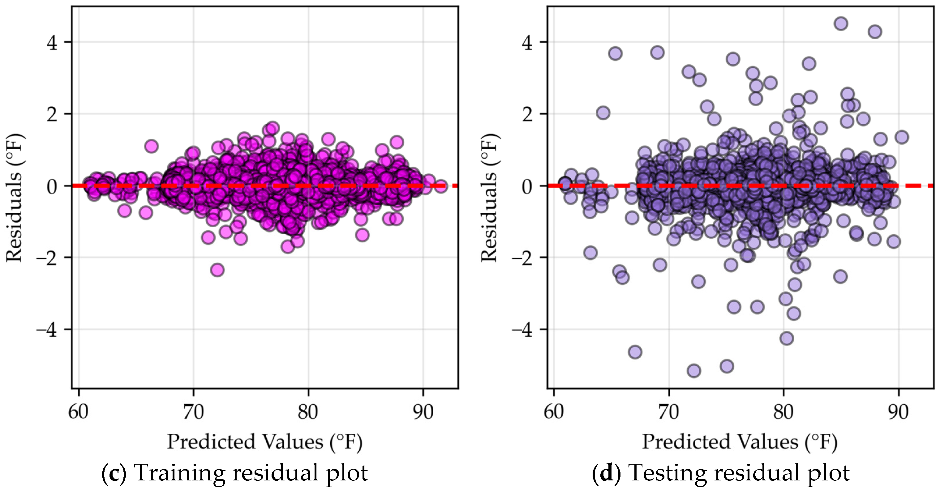
Gradient boosting was selected for its ability to handle complex datasets effectively, particularly in real-world scenarios with outliers or missing values. Additionally, gradient boosting integrates categorical and numerical data within a single framework, making it adaptable to various environments. For this analysis, extreme gradient boosting (XGBoost) was utilized over scikit-learn’s gradient boosting technique due to its superior performance. The key distinction between these implementations lies in their data-splitting techniques and regression tree construction [64]. XGBoost is a sophisticated model implemented through an open-source library aimed at being both efficient and effective, making it a preferred method for numerous applications [65].
Like all models, gradient boosting makes assumptions regarding the dataset structure. Figure 14 illustrates the model’s predictive process as additional trees are introduced. Sample 9 was accurately predicted after approximately 35 trees, while other data points, such as sample 424, required additional iterations to improve accuracy. However, as more trees were added to improve certain predictions, slight sacrifices in accuracy were made for previously well-predicted data points. This tradeoff is a common characteristic of boosting algorithms, where the model aims to minimize the overall average error rather than improving individual predictions.
When compared to the baseline MLR and neural network results, XGBoost consistently produced predictions that are closer to the true values. Figure 15 demonstrates this by showing that most data points are clustered near the central prediction line, indicating strong predictive ability. Although, unlike neural networks, which can capture more intricate data patterns, gradient boosting does not generalize as effectively. The model achieves acceptable error values but exhibits a noticeable performance gap between training and testing. Additionally, the dispersion of data points in testing does not always align with the patterns observed in training. For instance, in Figure 15c, data points around predicted temperature of 85 °F (29.4 °C) show minimal dispersion; while in Figure 15d, multiple outliers appear. Appendix A.4 provides an alternative visual of these outliers.
The discrepancy suggests that XGBoost, while effective, may exhibit some degree of overfitting, preventing it from identifying a fully generalized pattern. While it outperforms simpler models like MLR, it does not consistently achieve the same level of generalization as the neural network.

4.3.4. Bagging

Bagging was selected for its strong performance, particularly in reducing variance and mitigating the impact of incorrect data points [66]. However further improvements could be achieved by optimizing the number of subsets used. The best performing decision tree with a depth of three is listed in Figure 16, providing insight into how the model prioritizes inputs and makes predictions. These specific characteristic makes bagging highly suitable for HVAC applications, where occasional data inaccuracies may occur [47].
A comparison of residual and scatter plots highlights key differences between bagging and other models. In Figure 15, XGBoost displays a wider spread of data points compared to bagging in Figure 17. This suggests that XGBoost is more tolerant of errors but has greater dispersion, whereas bagging brings most predictions closer to expected values but struggles with outliers, leading to a wider spread of extreme residuals. This trade-off implies that bagging is better at capturing the general pattern of the dataset, whereas XGBoost maintains more flexibility in handling variations.
Additionally, Figure 17a,b show a similar dispersion pattern, suggesting that bagging is close to an optimal generalization of the data structure. However, differences in error values between training and testing indicate that the model does not fully capture the underlying pattern. Since the neural network successfully identified this pattern, it suggests a clear structure exists within the data that bagging does not fully exploit. While effective, bagging struggles with larger residuals compared to XGBoost, which sacrifices some generalization for better adaptability. Further pattern analysis for bagging is available in Appendix A.5.

4.3.5. Analysis of Model Specialties

Residual plot analysis reveals distinct differences in how each model processes the data. Neural networks excel at identifying patterns, XGBoost is more effective at handling outliers, and bagging strikes the best balance between these approaches. While their overall error values appear similar at a glance, a deeper evaluation is necessary to determine the most suitable model for practical applications.
In this study, bagging emerges as the most effective model, as supported by its error values. Its strength lies in capturing the underlying pattern while distinguishing true trends from noise, allowing it to make more reliable predictions. However, for further advancements, refining model parameters, particularly in neural networks, could lead to even better performance. Since the neural network demonstrated a strong ability to identify general patterns, optimizing its structure and parameters may yield superior results under more complex conditions.

5. Practical Application

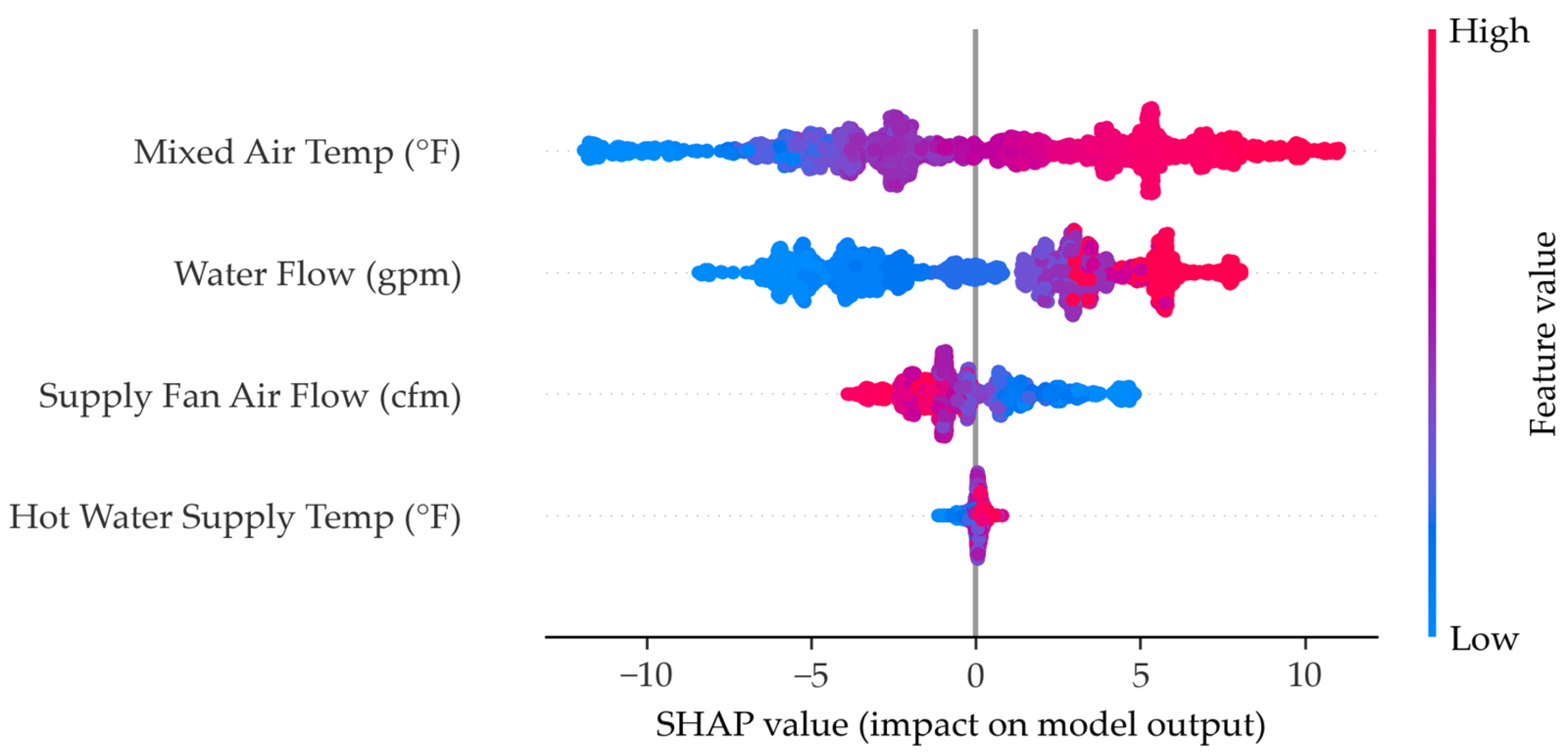
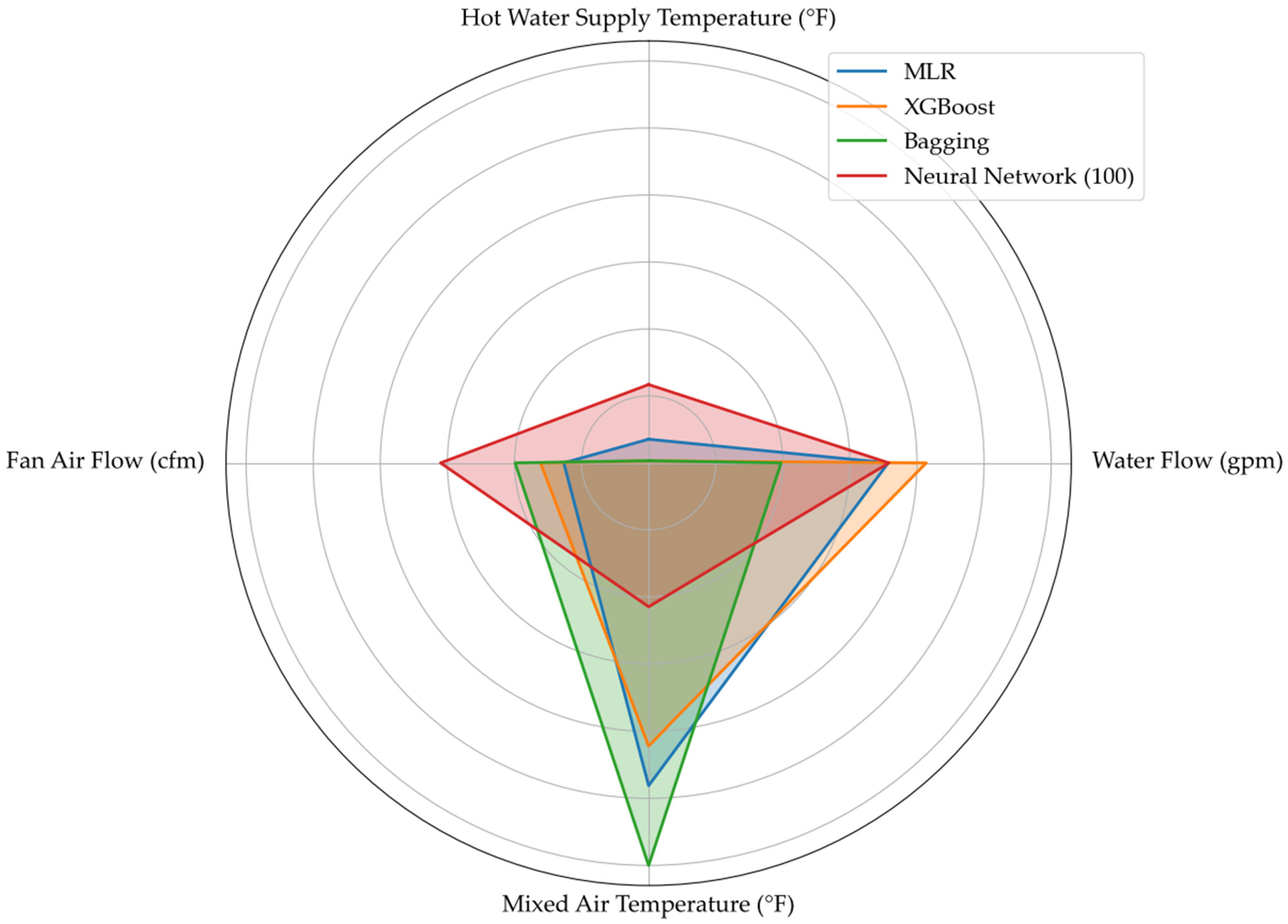
5.1. Input Significance

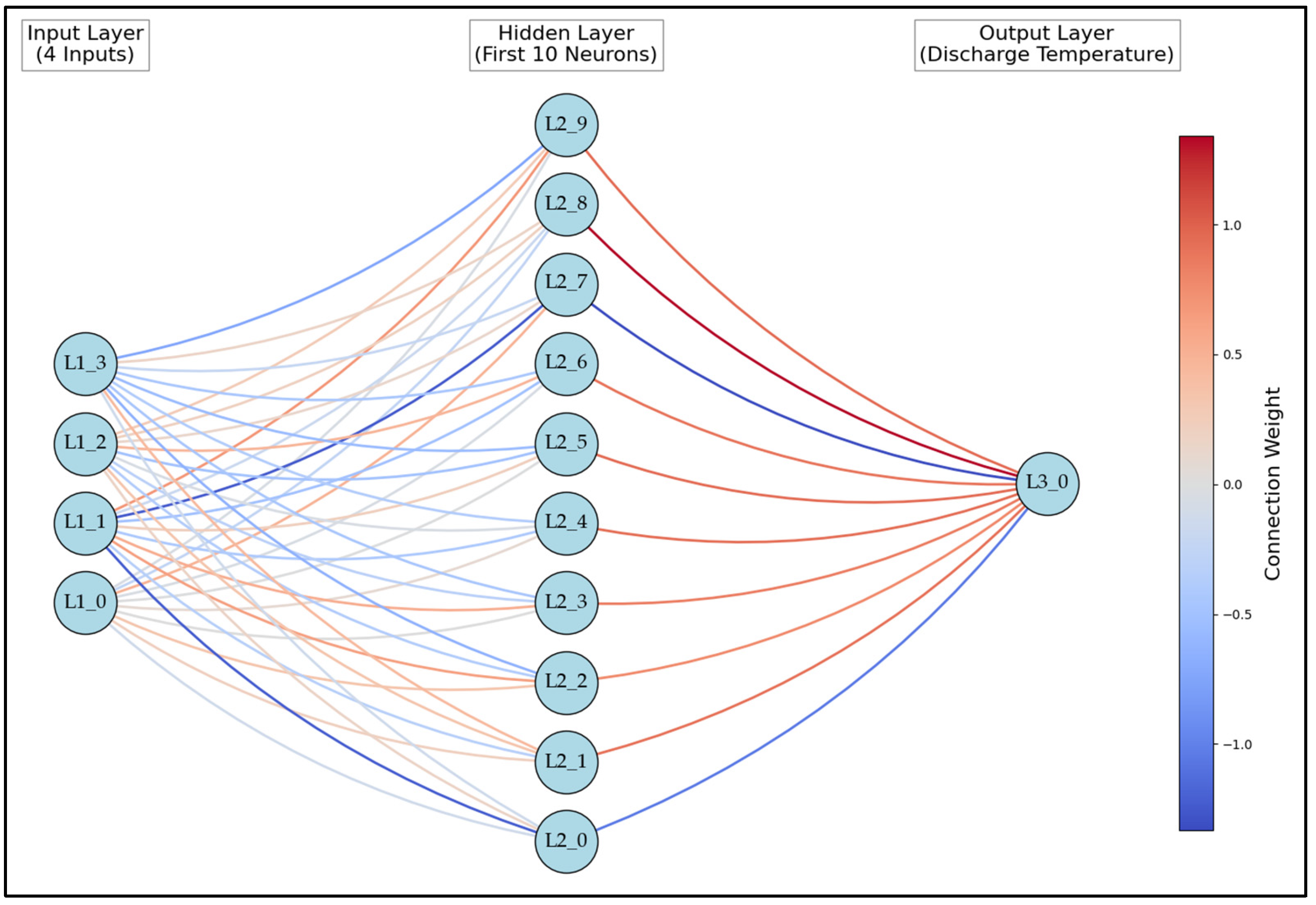
5.1.1. Model Input Weights

Each model assigned specific weights to the inputs, as illustrated in the radar chart below (Figure 18) and detailed in Table 2. The interpretation of these weights varies across models. MLR directly uses coefficients to quantify input significance, while XGBoost and bagging assess feature importance based on their contribution to predictive accuracy. Neural networks rely on connection weights between inputs and hidden layers, requiring node-level analysis for deeper insights.
A clearer comparison of how each model handles input weighting is provided in Appendix B, with specific distributions for MLR (Appendix B.1), neural networks (Appendix B.2), XGBoost (Appendix B.3), and bagging (Appendix B.4). These appendices offer a more detailed breakdown of model specific weighting approach, reinforcing these findings discussed in this section.
Despite differences in methodology, all models reached a similar conclusion regarding input significance. Hot water supply temperature was consistently identified as the least influential variable, while mixed air temperature emerged as the most critical factor.

5.1.2. Input Weight Considerations

Figure 19 and Figure 20 further examine the relationship between input variables for XGBoost and bagging. Notably, one visualization suggests that hot water temperature has subtle significance, seemingly contradicting previous assessments. This can be explained by the interaction between supply airflow rates and heating coil exposure time. When airflow decreases (i.e., fan speed is reduced), air remains in contact with the heating coil for a longer duration. As a result, lower hot water temperatures can achieve the same supply air temperatures compared to higher fan speeds.
Additionally, both models identified a negative correlation between supply airflow rate and supply air temperature. Higher airflow reduces heating time, leading to lower discharge air temperatures, while lower airflow extends exposure time, increasing heat absorption. However, in real-world applications, airflow rates cannot be freely adjusted due to ventilation and thermal comfort requirements. Excessive reductions in airflow may compromise air distribution and ventilation effectiveness, while excessive increases could cause pressure imbalances within the duct system. Understanding these constraints is crucial for applying model-driven optimizations to HVAC control strategies.

5.2. Model Applications

The developed heating coil models can be implemented in real-world building systems to monitor HVAC performance, detect anomalies, and enable proactive responses. One critical application is cybersecurity. These models can identify unauthorized control attempts or cyber-attacks on the HVAC system, ensuring that only authorized facility managers regulate building conditions. Such safeguards can help maintain a safe and healthy indoor environment for occupants.
Additionally, these models facilitate continuous monitoring of heating coil performance, allowing for real-time adjustments to optimize efficiency. By integrating them into energy management systems, facility managers can gain a comprehensive view of actual building performance, enabling data-driven decision-making. This integration supports the implementation of energy efficiency measures and helps identify operational inefficiencies, such as excessive energy use or suboptimal equipment settings.
Another key application is predictive maintenance. The models can forecast potential system failures, minimizing downtime and extending the lifespan of HVAC components by scheduling timely maintenance. During the design phase of new buildings, simulation-based models can guide the selection of appropriate system components and configurations. For existing buildings, these models support retrofit strategies aimed at enhancing performance and reducing energy consumption.
Given the broad range of applications, further refinement and expansion of these foundational models are paramount. Future research should focus on developing advanced control algorithms and extending modeling efforts to other critical HVAC components, such as reheating coils and chilled water coils, to enhance overall system performance and efficiency.

6. Conclusions

This study developed and evaluated predictive models for heating coil performance in HVAC systems, demonstrating that relatively simple models can achieve error thresholds sufficient for laboratory-scale applications. Among the tested models, bagging exhibited strong predictive accuracy, consistently performing well across analyzed error metrics, including R2, RMSE, MAE, MSE, and CV. It also demonstrated an ability to handle errors effectively and generalize patterns within the data. However, neural networks appeared to show greater potential for future advancements due to their strong performance in error metrics, capacity for developing more complex models, and ability to capture underlying patterns.
While these results highlight promising pathways for improving energy efficiency in HVAC systems, several limitations must be acknowledged. The experimental setup involved a small-scale unit operating under near-ideal conditions, which may not fully capture the complexities of real-world residential or commercial environments. Additionally, the study did not account for reheat and cooling coil loads or internal heat gains.
To enhance model robustness, future work should incorporate datasets from the entire HVAC system to find patterns all coils and operating parameters. This would enable the development of context-specific models, further optimizing energy efficiency across various implementation scenarios. Such advancements could significantly reduce global HVAC energy consumption, aligning with this study’s broader objectives of economic savings, ecological sustainability, and energy conservation.
While the current models perform well in controlled settings, their real-world applicability may be limited by unaccounted disturbances and inconsistencies in full-scale systems. Traditional machine learning models rely on mathematical formulations making them less effective at handling unstructured or illogical data without extensive human intervention for tuning and validation. In contrast, deep learning offers a transformative opportunity for HVAC predictive analytics. These models can be designed to simulate logical processes, allowing them to autonomously adapt to dynamic conditions, to identify logical inconsistencies, and to self-correct during operation. Future research should focus on optimizing deep learning parameters to develop more resilient, self-optimizing HVAC models capable of handling real-world variability with minimal manual oversight.

Author Contributions

Conceptualization, N.N. and P.D.; methodology, A.N. and P.D.; software, A.N.; validation, P.D., A.N. and N.N.; formal analysis, A.N.; investigation, A.N.; resources, A.N. and P.D.; data curation, P.D. and A.N.; writing—original draft preparation, A.N. and P.D.; writing—review and editing, P.D. and A.N.; visualization, A.N.; supervision, N.N. All authors have read and agreed to the published version of the manuscript.

Funding

This research received no external funding.

Data Availability Statement

Data used in this study are available upon request.

Conflicts of Interest

The authors declare no conflicts of interest.

Abbreviations

The following abbreviations are used in this manuscript:
AHUAir Handling Unit
HVACHeating Ventilation and Air Conditioning
BEASTBuilding Energy Assessments, Solutions, and Technologies
VAVVariable Air Volume
BASBuilding Automation System
ASHRAEAmerican Society of Heating Refrigerating and Air-Conditioning Engineers
MLRMultiple Linear Regression
XGBoostExtreme Gradient Boosting
R2Coefficient of determination
CVCoefficient of Variance
RMSERoot Mean Square Error
MSEMean Squared Error
MAEMean Absolute Error
SHAP Shapley Additive Explanations
ReLURectified Linear Unit

Appendix A. R2 and Residual Errors

Appendix A.1. R2 Values

The following graph shows the R2 values for the tested models. Blue lines represent testing R2, and orange lines shows training R2.
Figure A1. Testing vs. training R2 values of analyzed models.
Energies 18 02314 g0a1

Appendix A.2. MLR Predicted vs. Actual Data

The line plot presents a comparison between the predicted and actual values for MLR over samples 750–1250. The orange line represents the actual values, while the blue line represents the predicted values. Areas where the lines overlap indicate accurate predictions. Conversely, greater visibility of the blue line suggests a weaker model performance as it indicates a deviation between predicted and actual values.
Figure A2. MLR: actual vs. predictions.
Energies 18 02314 g0a2

Appendix A.3. Neural Network Predicted vs. Actual Data

The line plot shows a line graph connecting the values for the predicted data and actual data of the best-performing neural network for sample 750–1250.
Figure A3. Neural network: actual vs. predictions.
Energies 18 02314 g0a3

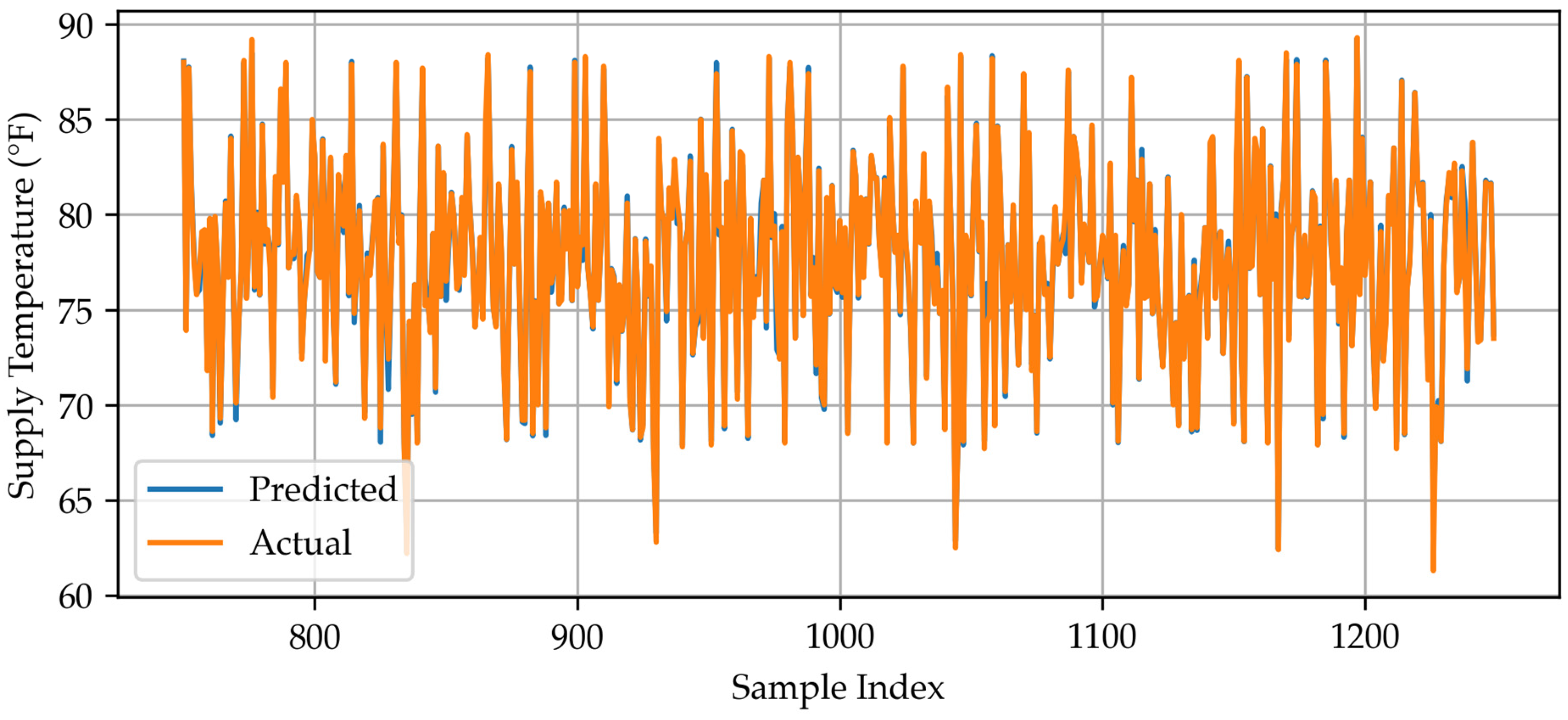
Appendix A.4. XGBoost Predicted vs. Actual Data

The line plot shows a line graph connecting the values for the predicted data and actual data of XGBoost for sample 750–1250.
Figure A4. XGBoost: actual vs. predictions.
Energies 18 02314 g0a4

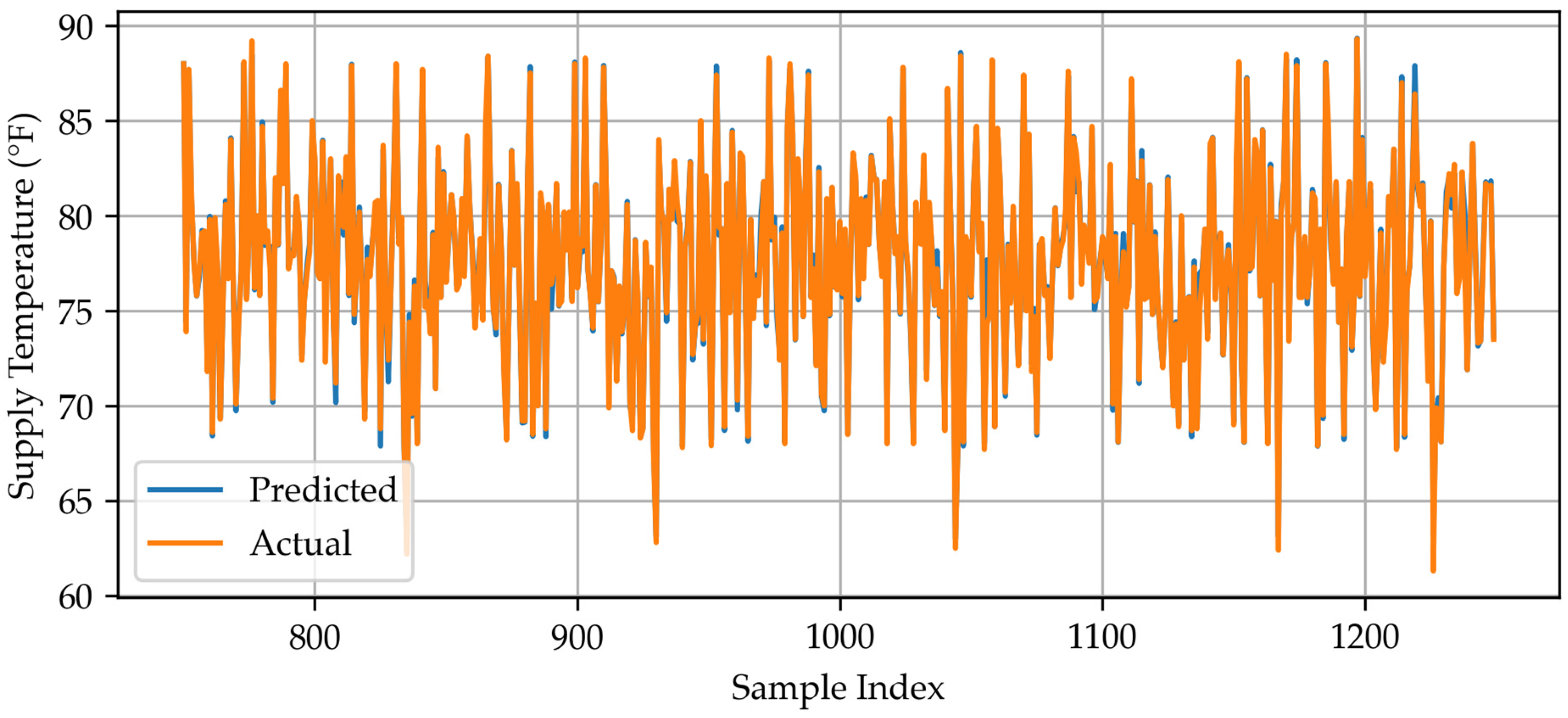
Appendix A.5. Bagging Predicted vs. Actual Data

The line plot shows a line graph connecting the values for the predicted data and actual data of bagging for sample 750–1250.
Figure A5. Bagging: actual vs. predictions.
Energies 18 02314 g0a5

Appendix B. Shapley Additive Explanations (SHAP) Values

Appendix B.1. MLR SHAP Chart

The SHAP chart for MLR visualizes the impact of each input variable on the model’s output. The y-axis represents the input features, while the x-axis shows their influence on predictions. Color gradients indicate the relative magnitude of each feature’s value across the dataset. A wider spread of data points suggests a stronger impact on the output, highlighting the most influential variables in the model.
Figure A6. MLR SHAP chart.
Energies 18 02314 g0a6

Appendix B.2. Neural Network SHAP Chart

SHAP chart for the best performing neural network.
Figure A7. Neural network SHAP chart.
Energies 18 02314 g0a7

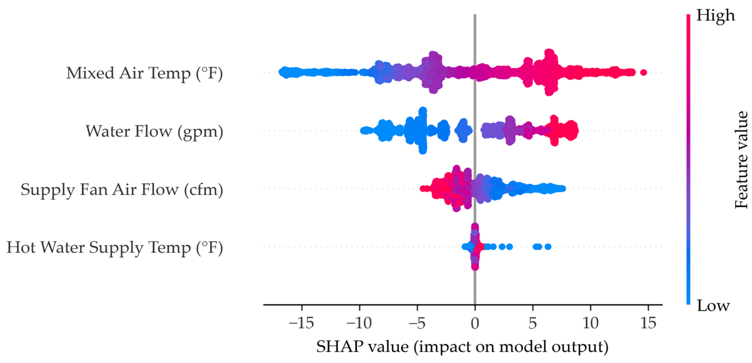
Appendix B.3. XGBoost SHAPSHAP Chart

SHAP chart for XGBoost.
Figure A8. XGBoost SHAP chart.
Energies 18 02314 g0a8

Appendix B.4. Bagging SHAP Chart

SHAP chart for bagging.
Figure A9. Bagging SHAP chart.
Energies 18 02314 g0a9

References

  1. Paul, W.L.; Taylor, P.A. A Comparison of Occupant Comfort and Satisfaction between a Green Building and a Conventional Building. Build. Environ. 2008, 43, 1858–1870. [Google Scholar] [CrossRef]
  2. Dharmasena, P.M.; Meddage, D.P.P.; Mendis, A.S.M. Investigating Applicability of Sawdust and Retro-Reflective Materials as External Wall Insulation under Tropical Climatic Conditions. Asian J. Civ. Eng. 2022, 23, 531–549. [Google Scholar] [CrossRef]
  3. Solano, J.C.; Caamaño-Martín, E.; Olivieri, L.; Almeida-Galárraga, D. HVAC Systems and Thermal Comfort in Buildings Climate Control: An Experimental Case Study. Energy Rep. 2021, 7, 269–277. [Google Scholar] [CrossRef]
  4. Dharmasena, P.; Nassif, N. Development and Optimization of a Novel Damper Control Strategy Integrating DCV and Duct Static Pressure Setpoint Reset for Energy-Efficient VAV Systems. Buildings 2025, 15, 518. [Google Scholar] [CrossRef]
  5. Westphalen, D.; Koszalinski, S. Energy Consumption Characteristics of Commercial Building HVAC Systems Volume I: Chillers, Refrigerant Compressors, and Heating Systems; Arthur D. Little, Inc.: Boston, MA, USA, 2001. [Google Scholar]
  6. American Socitey of Heating Ventilation and Air-Conditioning Systems and Equipment. 2020—ASHRAE Handbook—HVAC Systems and Equipment; ASHRAE: Peachtree Corners, GA, USA, 2020; ISBN 978-1-947192-52-2. [Google Scholar]
  7. U.S. Energy Information Administration (EIA). Use of Energy in Commercial Buildings. Available online: https://www.eia.gov/energyexplained/use-of-energy/commercial-buildings.php (accessed on 7 March 2025).
  8. Peters, G.P.; Andrew, R.M.; Canadell, J.G.; Friedlingstein, P.; Jackson, R.B.; Korsbakken, J.I.; Le Quéré, C.; Peregon, A. Carbon Dioxide Emissions Continue to Grow amidst Slowly Emerging Climate Policies. Nat. Clim. Change 2020, 10, 3–6. [Google Scholar] [CrossRef]
  9. Wang, Y.-W.; Cai, W.-J.; Soh, Y.-C.; Li, S.-J.; Lu, L.; Xie, L. A Simplified Modeling of Cooling Coils for Control and Optimization of HVAC Systems. Energy Convers. Manag. 2004, 45, 2915–2930. [Google Scholar] [CrossRef]
  10. Ebrahimi, P.; Ridwana, I.; Nassif, N. Solutions to Achieve High-Efficient and Clean Building HVAC Systems. Buildings 2023, 13, 1211. [Google Scholar] [CrossRef]
  11. Yu, B.; Kim, D.; Koh, J.; Kim, J.; Cho, H. Electrification and Decarbonization Using Heat Recovery Heat Pump Technology for Building Space and Water Heating. In Proceedings of the ASME 2023 17th International Conference on Energy Sustainability Collocated with the ASME 2023 Heat Transfer Summer Conference, Washington, DC, USA, 10–12 July 2023. [Google Scholar]
  12. Deason, J.; Borgeson, M. Electrification of Buildings: Potential, Challenges, and Outlook. Curr. Sustain. Renew. Energy Rep. 2019, 6, 131–139. [Google Scholar] [CrossRef]
  13. Yayla, A.; Świerczewska, K.S.; Kaya, M.; Karaca, B.; Arayici, Y.; Ayözen, Y.E.; Tokdemir, O.B. Artificial Intelligence (AI)-Based Occupant-Centric Heating Ventilation and Air Conditioning (HVAC) Control System for Multi-Zone Commercial Buildings. Sustainability 2022, 14, 16107. [Google Scholar] [CrossRef]
  14. Zhao, Y.; Li, T.; Zhang, X.; Zhang, C. Artificial Intelligence-Based Fault Detection and Diagnosis Methods for Building Energy Systems: Advantages, Challenges and the Future. Renew. Sustain. Energy Rev. 2019, 109, 85–101. [Google Scholar] [CrossRef]
  15. Babadi Soultanzadeh, M.; Ouf, M.M.; Nik-Bakht, M.; Paquette, P.; Lupien, S. Fault Detection and Diagnosis in Light Commercial Buildings’ HVAC Systems: A Comprehensive Framework, Application, and Performance Evaluation. Energy Build. 2024, 316, 114341. [Google Scholar] [CrossRef]
  16. ANSI/ASHRAE/IES Standard 90.1-2022; Energy Standard for Sites and Buildings Except Low-Rise Residential Buildings. American Socitey of Heating Ventilation and Air-Conditioning Systems and Equipment (ASHRAE): Peachtree Corners, GA, USA, 2022.
  17. International Code Council, Inc. (ICC). 2021 International Energy Conservation Code (IECC); ICC: Country Club Hills, IL, USA, 2021. [Google Scholar]
  18. The Paris Agreement|UNFCCC. Available online: https://unfccc.int/process-and-meetings/the-paris-agreement (accessed on 12 March 2025).
  19. Barney, G.C.; Florez, J. Temperature Prediction Models and Their Application to the Control of Heating Systems. IFAC Proc. Vol. 1985, 18, 1847–1852. [Google Scholar] [CrossRef]
  20. Asamoah, P.B.; Shittu, E. Evaluating the Performance of Machine Learning Models for Energy Load Prediction in Residential HVAC Systems. Energy Build. 2025, 334, 115517. [Google Scholar] [CrossRef]
  21. Lu, S.; Zhou, S.; Ding, Y.; Kim, M.K.; Yang, B.; Tian, Z.; Liu, J. Exploring the Comprehensive Integration of Artificial Intelligence in Optimizing HVAC System Operations: A Review and Future Outlook. Results Eng. 2025, 25, 103765. [Google Scholar] [CrossRef]
  22. Gao, Z.; Yu, J.; Zhao, A.; Hu, Q.; Yang, S. A Hybrid Method of Cooling Load Forecasting for Large Commercial Building Based on Extreme Learning Machine. Energy 2022, 238, 122073. [Google Scholar] [CrossRef]
  23. Norouzi, P.; Maalej, S.; Mora, R. Applicability of Deep Learning Algorithms for Predicting Indoor Temperatures: Towards the Development of Digital Twin HVAC Systems. Buildings 2023, 13, 1542. [Google Scholar] [CrossRef]
  24. Maddalena, E.T.; Lian, Y.; Jones, C.N. Data-Driven Methods for Building Control—A Review and Promising Future Directions. Control Eng. Pract. 2020, 95, 104211. [Google Scholar] [CrossRef]
  25. Halhoul Merabet, G.; Essaaidi, M.; Ben Haddou, M.; Qolomany, B.; Qadir, J.; Anan, M.; Al-Fuqaha, A.; Abid, M.R.; Benhaddou, D. Intelligent Building Control Systems for Thermal Comfort and Energy-Efficiency: A Systematic Review of Artificial Intelligence-Assisted Techniques. Renew. Sustain. Energy Rev. 2021, 144, 110969. [Google Scholar] [CrossRef]
  26. Platt, G.; Li, J.; Li, R.; Poulton, G.; James, G.; Wall, J. Adaptive HVAC Zone Modeling for Sustainable Buildings. Energy Build. 2010, 42, 412–421. [Google Scholar] [CrossRef]
  27. Zhang, C.; Zhao, Y.; Fan, C.; Li, T.; Zhang, X.; Li, J. A Generic Prediction Interval Estimation Method for Quantifying the Uncertainties in Ultra-Short-Term Building Cooling Load Prediction. Appl. Therm. Eng. 2020, 173, 115261. [Google Scholar] [CrossRef]
  28. Ding, Y.; Zhang, Q.; Wang, Z.; Liu, M.; He, Q. A Simplified Model of Dynamic Interior Cooling Load Evaluation for Office Buildings. Appl. Therm. Eng. 2016, 108, 1190–1199. [Google Scholar] [CrossRef]
  29. Lin, X.; Tian, Z.; Lu, Y.; Zhang, H.; Niu, J. Short-Term Forecast Model of Cooling Load Using Load Component Disaggregation. Appl. Therm. Eng. 2019, 157, 113630. [Google Scholar] [CrossRef]
  30. Dharmasena, P.; Nassif, N. Testing, Validation, and Simulation of a Novel Economizer Damper Control Strategy to Enhance HVAC System Efficiency. Buildings 2024, 14, 2937. [Google Scholar] [CrossRef]
  31. Wahba, N.; Rismanchi, B.; Pu, Y.; Aye, L. Efficient HVAC System Identification Using Koopman Operator and Machine Learning for Thermal Comfort Optimisation. Build. Environ. 2023, 242, 110567. [Google Scholar] [CrossRef]
  32. Babadi Soultanzadeh, M.; Nik-Bakht, M.; Ouf, M.M.; Paquette, P.; Lupien, S. Unsupervised Automated Fault Detection and Diagnosis for Light Commercial Buildings’ HVAC Systems. Build. Environ. 2025, 267, 112312. [Google Scholar] [CrossRef]
  33. Chen, Z.; Xu, P.; Feng, F.; Qiao, Y.; Luo, W. Data Mining Algorithm and Framework for Identifying HVAC Control Strategies in Large Commercial Buildings. Build. Simul. 2021, 14, 63–74. [Google Scholar] [CrossRef]
  34. Khanuja, A.; Webb, A.L. What We Talk about When We Talk about EEMs: Using Text Mining and Topic Modeling to Understand Building Energy Efficiency Measures (1836-RP). Sci. Technol. Built Environ. 2023, 29, 4–18. [Google Scholar] [CrossRef]
  35. Ajifowowe, I.; Chang, H.; Lee, C.S.; Chang, S. Prospects and Challenges of Reinforcement Learning-Based HVAC Control. J. Build. Eng. 2024, 98, 111080. [Google Scholar] [CrossRef]
  36. Jiang, M.L.; Wu, J.Y.; Xu, Y.X.; Wang, R.Z. Transient Characteristics and Performance Analysis of a Vapor Compression Air Conditioning System with Condensing Heat Recovery. Energy Build. 2010, 42, 2251–2257. [Google Scholar] [CrossRef]
  37. Wang, S.; Ma, Z. Supervisory and Optimal Control of Building HVAC Systems: A Review. Hvac&R Res. 2008, 14, 3–32. [Google Scholar] [CrossRef]
  38. Belany, P.; Hrabovsky, P.; Sedivy, S.; Cajova Kantova, N.; Florkova, Z. A Comparative Analysis of Polynomial Regression and Artificial Neural Networks for Prediction of Lighting Consumption. Buildings 2024, 14, 1712. [Google Scholar] [CrossRef]
  39. Fumo, N.; Rafe Biswas, M.A. Regression Analysis for Prediction of Residential Energy Consumption. Renew. Sustain. Energy Rev. 2015, 47, 332–343. [Google Scholar] [CrossRef]
  40. 6.1—MLR Model Assumptions|STAT 462. Available online: https://online.stat.psu.edu/stat462/node/145/ (accessed on 19 March 2025).
  41. Lee, C.-W.; Fu, M.-W.; Wang, C.-C.; Azis, M.I. Evaluating Machine Learning Algorithms for Financial Fraud Detection: Insights from Indonesia. Mathematics 2025, 13, 600. [Google Scholar] [CrossRef]
  42. Abiodun, O.I.; Jantan, A.; Omolara, A.E.; Dada, K.V.; Mohamed, N.A.; Arshad, H. State-of-the-Art in Artificial Neural Network Applications: A Survey. Heliyon 2018, 4, e00938. [Google Scholar] [CrossRef]
  43. Han, S.-H.; Kim, K.W.; Kim, S.; Youn, Y.C. Artificial Neural Network: Understanding the Basic Concepts Without Mathematics. Dement. Neurocogn Disord. 2018, 17, 83–89. [Google Scholar] [CrossRef]
  44. 1.17.Neural Network Models (Supervised). Available online: https://scikit-learn.org/stable/modules/neural_networks_supervised.html (accessed on 19 March 2025).
  45. Abdolrasol, M.G.M.; Hussain, S.M.S.; Ustun, T.S.; Sarker, M.R.; Hannan, M.A.; Mohamed, R.; Ali, J.A.; Mekhilef, S.; Milad, A. Artificial Neural Networks Based Optimization Techniques: A Review. Electronics 2021, 10, 2689. [Google Scholar] [CrossRef]
  46. Engelbrecht, A.P.; Cloete, I.; Zurada, J.M. Determining the Significance of Input Parameters Using Sensitivity Analysis. In Proceedings of the From Natural to Artificial Neural Computation, Torremolinos, Spain, 7–9 June 1995; Mira, J., Sandoval, F., Eds.; Springer: Berlin/Heidelberg, Germany, 1995; pp. 382–388. [Google Scholar]
  47. Breiman, L. Bagging Predictors. Mach. Learn. 1996, 24, 123–140. [Google Scholar] [CrossRef]
  48. Dietterich, T.G. Machine-Learning Research. AI Mag. 1997, 18, 97–136. [Google Scholar] [CrossRef]
  49. Friedman, J.H. Greedy Function Approximation: A Gradient Boosting Machine. Ann. Stat. 2001, 29, 1189–1232. [Google Scholar] [CrossRef]
  50. Nogales, A.G. On Consistency of the Bayes Estimator of the Density. Mathematics 2022, 10, 636. [Google Scholar] [CrossRef]
  51. Gu, M.; Kang, S.; Xu, Z.; Lin, L.; Zhang, Z. AE-XGBoost: A Novel Approach for Machine Tool Machining Size Prediction Combining XGBoost, AE and SHAP. Mathematics 2025, 13, 835. [Google Scholar] [CrossRef]
  52. Scikit-Learn: Machine Learning in Python—Scikit-Learn 1.6.1 Documentation. Available online: https://scikit-learn.org/stable/ (accessed on 12 March 2025).
  53. Pandas—Python Data Analysis Library. Available online: https://pandas.pydata.org/ (accessed on 12 March 2025).
  54. NumPy. Available online: https://numpy.org/ (accessed on 12 March 2025).
  55. Li, X.; Shen, Y.; Meng, Q.; Xing, M.; Zhang, Q.; Yang, H. Single-Model Self-Recovering Fringe Projection Profilometry Absolute Phase Recovery Method Based on Deep Learning. Sensors 2025, 25, 1532. [Google Scholar] [CrossRef]
  56. Jakubec, M.; Cingel, M.; Lieskovská, E.; Drliciak, M. Integrating Neural Networks for Automated Video Analysis of Traffic Flow Routing and Composition at Intersections. Sustainability 2025, 17, 2150. [Google Scholar] [CrossRef]
  57. James, G.; Witten, D.; Hastie, T.; Tibshirani, R. An Introduction to Statistical Learning: With Applications in R; Springer Texts in Statistics; Springer: New York, NY, USA, 2021; ISBN 978-1-0716-1417-4. [Google Scholar]
  58. Qavidelfardi, Z.; Tahsildoost, M.; Zomorodian, Z.S. Using an Ensemble Learning Framework to Predict Residential Energy Consumption in the Hot and Humid Climate of Iran. Energy Rep. 2022, 8, 12327–12347. [Google Scholar] [CrossRef]
  59. Wang, J.; Yuan, Z.; He, Z.; Zhou, F.; Wu, Z. Critical Factors Affecting Team Work Efficiency in BIM-Based Collaborative Design: An Empirical Study in China. Buildings 2021, 11, 486. [Google Scholar] [CrossRef]
  60. Neter, J.; Wasserman, W.; Kutner, M.H. Applied Linear Regression Models; Richard D. Irwin, Inc.: Homewood, IL, USA, 1983; ISBN 0-256-02547-9. [Google Scholar]
  61. Lian, J.; Jiang, J.; Dong, X.; Wang, H.; Zhou, H.; Wang, P. Coupled Motion Characteristics of Offshore Wind Turbines During the Integrated Transportation Process. Energies 2019, 12, 2023. [Google Scholar] [CrossRef]
  62. Liu, J.; Wu, Q.; Sui, X.; Chen, Q.; Gu, G.; Wang, L.; Li, S. Research Progress in Optical Neural Networks: Theory, Applications and Developments. PhotoniX 2021, 2, 5. [Google Scholar] [CrossRef]
  63. Babatunde, D.E.; Anozie, A.; Omoleye, J. Artificial Neural Network and Its Applications in the Energy Sector—An Overview. Int. J. Energy Econ. Policy 2020, 10, 250–264. [Google Scholar] [CrossRef]
  64. XGBoost Documentation—Xgboost 3.0.0 Documentation. Available online: https://xgboost.readthedocs.io/en/stable/ (accessed on 25 March 2025).
  65. Chen, T.; Guestrin, C. XGBoost: Reliable Large-Scale Tree Boosting System. In Proceedings of the 22nd SIGKDD Conference on Knowledge Discovery and Data Mining, San Francisco, CA, USA, 13–17 August 2016. [Google Scholar]
  66. Sehrawat, N.; Vashisht, S.; Singh, A. Solar Irradiance Forecasting Models Using Machine Learning Techniques and Digital Twin: A Case Study with Comparison. Int. J. Intell. Netw. 2023, 4, 90–102. [Google Scholar] [CrossRef]
Figure 1. Typical AHU and major components.
Energies 18 02314 g001
Figure 2. Common activation functions in neural networks.
Energies 18 02314 g002
Figure 3. Neural network loss function over iterations.
Energies 18 02314 g003
Figure 4. Common neural network architectural shapes.
Energies 18 02314 g004
Figure 5. Schematic of the bagging process.
Energies 18 02314 g005
Figure 6. Schematic of the gradient boosting process (color changes indicates updates at each stage).
Energies 18 02314 g006
Figure 7. Gradient descent on a 3D loss surface.
Energies 18 02314 g007
Figure 8. Overall workflow of the research.
Energies 18 02314 g008
Figure 9. BEAST laboratory facility and tested equipment.
Energies 18 02314 g009
Figure 10. Training and testing R2 for evaluated models.
Energies 18 02314 g010
Figure 11. MLR residual and scatter plots.
Energies 18 02314 g011
Figure 12. Neural network connection weights.
Energies 18 02314 g012
Figure 13. Neural network residual and scatter plots.
Energies 18 02314 g013
Figure 14. Predicted accumulation of samples for XGBoost.
Energies 18 02314 g014
Figure 15. XGBoost residual and scatter plots.
Energies 18 02314 g015aEnergies 18 02314 g015b
Figure 16. Bagging tree with max depth 3.
Energies 18 02314 g016
Figure 17. Bagging residual and scatter plots.
Energies 18 02314 g017
Figure 18. Relative input weights for the models.
Energies 18 02314 g018
Figure 19. XGBoost input relationships.
Energies 18 02314 g019
Figure 20. Bagging input relationships.
Energies 18 02314 g020
Table 1. Error values from uncleaned dataset.
Error Values
ModelsR2 TrainR2 TestRMSEMAEMSECV
Bagging0.9978540.9770270.7619060.2916030.5805000.980804
Random Forest0.9978670.9769290.7635340.2910760.5829850.982900
Voting Regressor0.9949690.9766030.7689070.3216400.5912180.989816
XGBoost0.9975640.9746970.7996100.3272230.6393761.029341
Table 2. Input weights for models.
Models
Input ValuesMLRNeural Network (100)BaggingXGBoost
Hot Water Supply Temperature (°F)0.0350.1170.0030.003
Water Flow (gpm)0.3570.3580.1970.414
Mixed Air Temperature (°F)0.4810.2150.6000.422
Supply Fan Air Flow (cfm)0.1260.3100.1990.161
Disclaimer/Publisher’s Note: The statements, opinions and data contained in all publications are solely those of the individual author(s) and contributor(s) and not of MDPI and/or the editor(s). MDPI and/or the editor(s) disclaim responsibility for any injury to people or property resulting from any ideas, methods, instructions or products referred to in the content.

