Hybrid Method for Oil Price Prediction Based on Feature Selection and XGBOOST-LSTM

Abstract

The accurate and stable prediction of crude oil prices holds significant value, providing insightful guidance for investors and decision-makers. The intricate interplay of factors influencing oil prices and the pronounced fluctuations present significant obstacles within the realm of oil price forecasting. This study introduces a novel hybrid model framework, distinct from the conventional methods, that integrates influencing factors for oil price prediction. First, using Improved Complete Ensemble Empirical Mode Decomposition with Adaptive Noise (ICEEMDAN) extract mode components from crude oil prices. Second, using the Adaptive Copula-based Feature Selection (ACBFS), rooted in Copula theory, facilitates the integration of the influencing factors; ACBFS enhances both accuracy and stability in feature selection, thereby amplifying predictive performance and interpretability. Third, low-frequency modes are predicted through an Attention Mechanism-based Long and Short-Term Memory Neural Network (AM-LSTM), optimized using Bayesian Optimization and Hyperband (BOHB). Conversely, high-frequency modes are forecasted using Extreme Gradient Boosting Models (XGboost). Finally, the error correction mechanism further enhances the predictive accuracy. The experimental results show that the Mean Absolute Error (MAE) and Root Mean Square Error (RMSE) of the proposed hybrid prediction framework are the lowest compared to the benchmark model, at 0.7333 and 1.1069, respectively, which proves that the designed prediction structure has better efficiency and higher accuracy and stability.

1. Introduction

Energy serves as the foundation and driving force behind the advancement of human civilization. Throughout the course of human development, energy has assumed a vital role as the lifeblood of industry and the cornerstone of the national economy. It is an indispensable element for facilitating rapid economic growth and ensuring the enduring stability of society. Crude oil, a non-renewable energy resource, finds extensive utility in the progress of modern industry. Referred to as the “lifeblood of industry,” it has significantly contributed to the evolution of the global economy. The BP Statistical Yearbook of World Energy [1], published in 2022, underscores crude oil’s preeminent role by accounting for a largest share of energy consumption within the global energy mix. Crude oil prices are at the centre of the crude oil market and key to ensuring stability in the energy market.

In recent years, the distinctive attributes of crude oil have significantly heightened the focus on the volatility and trajectory of international oil prices [2]. The fluctuation of international oil prices not only reflects the trajectory of global economic development, but is also closely linked to fundamental societal issues within individual countries. Therefore, accurate oil price forecasting is important for energy security, economic decision-making, and financial market stability, and is a crucial basis for the formulation of effective policies and investment strategies [3]. However, due to the complexity of and non-stationarity in the oil price series [4], the volatility of oil prices is affected by a range of external factors [5], and these challenges increase the difficulty in achieving accurate oil price predictions. Furthermore, machine learning or deep learning models have become the mainstream of oil price prediction [6], and their powerful non-linear processing ability makes them have better prediction performance compared with the traditional linear models [7]. However, there are a large number of hyperparameters in deep learning, and inappropriate parameter settings may lead to performance degradation [8]. How to obtain the appropriate parameters to improve the fitness of the model and the data is still an open problem. Based on this, this study proposes a hybrid oil price forecasting framework to address these challenges. Improved Complete Ensemble Empirical Mode Decomposition with Adaptive Noise (ICEEMDAN) is used to extract the mode components in the oil price to overcome the complexity of the series. Then, the influences of different modes are screened to determine the optimal input features and time lag steps based on an advanced feature extraction algorithm, Adaptive Copula-based Feature Selection (ACBFS). Furthermore, combining the advantages of different models, such as the Attention Mechanism-based Long and Short-Term Memory Neural Network (AM-LSTM), predicts low-frequency modes, and Extreme Gradient Boosting Models (XGBoost) can be used for the prediction of high-frequency modes. The hyperparameters in the model were tuned using Bayesian Optimization and Hyperband (BOHB). Finally, this study introduces an error correction mechanism to further enhance the prediction accuracy. The experimental results prove that the hybrid prediction framework proposed in this study can solve the current challenges being faced in oil price prediction to a certain extent, and the main contributions of this study are as follows:

(1) This study proposes an oil price prediction framework that combines ICEEMDAN decomposition and mode–feature matching modelling, introduces the XGBoost model to improve the stability of prediction for the highly fluctuating characteristics of high-frequency modes, and adopts the AM-LSTM deep learning model for the smooth trend of low-frequency modes, which effectively enhances the adaptability and robustness of the prediction model to the non-linear and non-smooth features;

(2) By introducing the ACBFS method to achieve the dynamic screening and fusion of input features, the model’s ability to handle multidimensional features is enhanced, while by combining with the attention mechanism, key feature information is effectively extracted, and the interpretability and predictive performance of the feature selection process is improved;

(3) The BOHB algorithm is used to optimize the hyperparameters to enhance the robustness of the model. Meanwhile, the residual sequences are modelled to correct the potential systematic prediction errors and overcome the shortcomings of the traditional methods that generally ignore the non-white noise characteristics of the residuals, and to further improve the prediction accuracy.

2. Literature Review

Traditional econometrics and machine learning are the main models of choice in oil price forecasting. Econometric models depend on linearity assumptions and are mainly used for volatility analyses of oil prices [9,10] and spillover effects [11]. It is highly self-explanatory, however, that the complexity and non-linearity of oil prices [12] often lead to econometric models’ poor predictive performance. Machine learning is beginning to be widely used for oil price prediction due to its powerful non-linear fitting ability. Huang and Wang (2018) used artificial neural networks (ANNs) to predict two international crude oil prices, and the experimental results proved the powerful prediction performance of ANN [13]. Cen and Wang (2019) predicted crude oil prices based on a Long Short-Term Memory neural network (LSTM), and the LSTM showed high accuracy in several datasets [7]. In addition, many other machine learning models have been shown to have excellent predictive power in oil price forecasting [14,15]. The above study validates the effectiveness of machine learning models for oil price prediction. However, the predictive ability of individual models is often limited [16]. Researchers are beginning to combine multiple models to build hybrid frameworks to further improve prediction accuracy. Common hybrid models fall into three main categories: the first category is the fusion of optimization algorithms with predictive models, involving the utilization of optimization algorithms such as Particle Swarm Optimization (PSM) [17] or Bayesian optimization [18], etc., to fine-tune the hyperparameters of predictive models or optimize the objective function, thereby enhancing model performance [19,20]; the second category involves the amalgamation of diverse prediction models to synthesize their predictive outcomes [21,22]; and the third category introduces signal decomposition algorithms, which dissect the raw data into multiple sub-models, each corresponding to distinct features or components of the data [23,24,25,26,27]. Decomposition methods better capture latent structures and features within the data, thereby elevating the model’s performance. While the initial two hybrid models may leverage their unique advantages to enhance predictive accuracy, inappropriate model selection can lead to modelling difficulties. Bayesian optimization tends to consume significant computational resources [28], and heuristic algorithms may lead to the non-convergence of optimization results [29]. In addition, they may have difficulty in modelling the characteristics of crude oil price volatility, leading to the overfitting of the model. Although the decomposition-integrated prediction model can yield favourable results, its efficacy remains subject to the influence of its constituent components. The commonly used empirical mode decomposition (EMD-based method) can lead to mode aliasing problems [30]. Consequently, the judicious selection of the predictive model assumes paramount importance in the pursuit of heightened prediction accuracy.

Furthermore, the intricate trajectory of crude oil prices is significantly impacted by a constellation of multifarious determinants, including but not limited to geopolitical intricacies, economic dynamics, and the pricing dynamics of substitute commodities [31,32]. Within the purview of energy policy formulation, the forecasting of crude oil prices anchored in a nuanced consideration of these manifold influencing factors assumes pivotal significance. Consequently, the development of a robust crude oil price forecasting model capable of accommodating these diverse influences constitutes a formidable and imperative scholarly endeavour. Zhai et al. (2025) used deep learning techniques to model the factors influencing oil price, and the experimental results showed that the prediction accuracy of oil price predictions was improved after incorporating multidimensional features [33]. Tao et al. (2025) used multivariate empirical mode decomposition (MEMD) for the multidimensional decomposition of the factors affecting oil price, and thus improved prediction accuracy [34]. However, more modelling factors increase the risk of model overfitting [35], which can negatively affect model accuracy. Therefore, some researchers have adopted feature engineering to screen important features, and the commonly used methods include correlation coefficient [36], mutual information entropy [37], and random forest [38]. However, while these methods are able to quantify the correlation information between the predicted data and each feature, there are currently no explicit quantitative criteria for determining the correct number of feature sets [39].

Based on the above literature review, there are still some challenges in oil price forecasting, including how to select complex multidimensional features and construct a more appropriate and robust hybrid prediction model. To address these issues, this study proposes a novel hybrid prediction framework that integrates signal decomposition, feature selection, and machine learning–deep learning fusion. Specifically, ICEEMDAN is used to decompose the original oil price series into intrinsic mode functions, capturing the non-linear and non-stationary characteristics of the data more accurately [40]. ACBFS is adopted to perform adaptive feature selection by dynamically filtering complementary information across modes, thus enhancing model interpretability and prediction robustness [39]. In the modelling stage, XGBoost is applied to high-frequency components with strong fluctuations, while AM-LSTM is used for low-frequency components with smoother trends [41]. The attention mechanism further improves the ability of the model to focus on key features [42]. To enhance optimization efficiency, BOHB, which has a shorter running time and faster convergence compared to Bayesian optimization, is employed for hyperparameter tuning [18]. Moreover, to account for non-white noise in prediction residuals [43], an error correction mechanism is incorporated to further improve the final forecasting performance [44].

3. Methodology

3.1. Model Framework

The hybrid model framework proposed in this study is shown in Figure 1. First, this study uses ICEEMDAN to decompose the original oil price series. ICEEMDAN can overcome the problems in EMD, EEMD, and CEEMDAN to obtain smoother and more stable modal features. Second, the optimal input features and lag steps for different IMFs are obtained via ACBFS; these features are concatenated with different modes to obtain the inputs of the model. Furthermore, AM-LSTM was used for the prediction of low-frequency modes, while XGBoost was used for the prediction of high-frequency modes, and BOHB optimized the hyperparameters in the model during the prediction modelling process. Subsequently, oil price predictions are obtained by summing the predictions of the high- and low-frequency modes. Finally, this study introduces the error correction mechanism, which improves the prediction performance of the model by predicting the residuals.

3.2. ICEEMDAN

EMD is able to adaptively analyze linear and non-linear and smooth and non-smooth models [45], and is widely used in prediction models, but when there are abrupt, disturbing signals in the signal, the EMD decomposition results may have mode aliasing [46], which will make the IMF impractical and cannot show the characteristics of the time series. While EEMD [47] adds a large amount of Gaussian white noise to EMD to solve the problem of modal aliasing, the reconstructed sequence may not be equal to the original sequence. CEEMDAN [48] solves the problem of the EEMD algorithm by generating spurious components to a certain extent. In practical engineering applications, CEEMDAN decomposition results in residual noise, leading to the contamination of the IMF. Compared to CEEMDAN, ICEEMDAN further optimizes the noise addition by adaptively adjusting the amplitude and structure of the added noise according to the current local characteristics of the signal to be decomposed, and furthermore, ICEEMDAN improves the stability and the accuracy of the IMF extraction process by extracting the local average trend of multiple noise-added samples, followed by a unified intrinsic-mode decomposition [49]. The steps of ICEEMDAN are as follows:

Step (1): Add Gaussian white noise $\tilde{\overline{X}}(t)~N\left(0,1\right)$ to the original sequence ${\tilde{\epsilon }}^{\omega }(t)$, and the original series becomes a new sequence ${\tilde{\overline{x}}}^i(t)=\tilde{\overline{x}}(t)+{\beta }_0{\tilde{\overline{\epsilon }}}^{(i)}(t)$. Subsequently, decompose the new sequence using the EMD algorithm to obtain the first remaining component ${\overline{\overline{\Omega }}}_1(t)$ after I trials:

$${\overline{\overline{\Omega }}}_1(t)=⟨Mean\left({\tilde{\overline{X}}}^{(i)}(t)\right)⟩$$

(1)

The $Mean(·)$ is the operator that computes the local mean of the sequence with $E_1\left(\tilde{\overline{X}}(t)\right)=\tilde{\overline{X}}(t)-Mean\left({\tilde{\overline{X}}}^{(i)}(t)\right)$.

Step (2): The first intrinsic modal component IMF₁(n) is computed based on the residual component ${\overline{\overline{\Omega }}}_1(t)$ obtained in the previous step:

$$IM{F}_1(n)=\tilde{\overline{X}}(t)-{\overline{\overline{\Omega }}}_1(t)$$

(2)

Step (3): Estimate the residual component ${\overline{\overline{\Omega }}}_2(t)={\overline{\overline{\Omega }}}_1(t)+{\beta }_1{E}_2\left({\tilde{\overline{\epsilon }}}^{(i)}(t)\right)$ from ${\overline{\overline{\Omega }}}_1(t)$ and operator $E(·)$, from which the next intrinsic modal component IMF2(n) is calculated:

$$IM{F}_2(n)={\overline{\overline{\Omega }}}_1(t)-⟨Mean\left({\overline{\overline{\Omega }}}_1(t)+{\beta }_1{E}_2\left({\tilde{\overline{\epsilon }}}^{(i)}(t)\right)\right)⟩$$

(3)

Step (4): Computing the kth residual component ${\overline{\overline{\Omega }}}_k(t)$, where k = 3, 4, …, K:

$${\overline{\overline{\Omega }}}_k\left(t\right)=⟨Mean\left({\overline{\overline{\Omega }}}_{k-1}(t)+{\beta }_{k-1}{E}_k\left({\tilde{\overline{\epsilon }}}^{(i)}(t)\right)\right)⟩$$

(4)

Step (5): Calculating the kth intrinsic modal component IMFk(n):

$$IM{F}_k(n)={\overline{\overline{\Omega }}}_{k-1}(t)-{\overline{\overline{\Omega }}}_k(t)$$

(5)

Step (6): Repeating the above steps until the termination condition is satisfied, obtaining K intrinsic modal components as well as $\overline{\overline{\Omega }}(t)$. At this point, the original time series $\tilde{\overline{X}}(t)$ is decomposed into the following:

$$\tilde{\overline{X}}(t)={\sum }_{k=1}^{K}IM{F}_k(t)+\overline{\Omega }(t)$$

(6)

3.3. ACBFS

ACBFS is a Copula-based adaptive feature selection method for data analysis and feature engineering. The goal of ACBFS is to select the most relevant and predictive features from the original set of features to improve the performance of the model and reduce the redundant information.

The Copula function, also known as the connectivity function, was first proposed by Sklar’s theorem [50]: assuming that X₁, X₂, …, X_n are n random variables with their respective marginal distribution functions F₁(x₁), F₂(x₂), …, F_n(x_n), and the joint distribution function F(x₁, x₂,…, x_n), then there is a Copula function C (·) such that

$$F(x_1,x_2,\dots ,x_n)=C\left(F_1\left(x_1\right),F_2\left(x_2\right),\dots ,F_n\left(x_n\right)\right)$$

(7)

Let C denote the Copula density function, and the nth order partial derivative of this joint distribution function gives the following expression:

$$f(x_1, x_2, \dots ,x_n)=c\left(F_1(x_1), F_2(x_2), \dots , F_n(x_n)\right)\prod _i{f}_i(x_i)$$

(8)

Both mutual information and information entropy are important concepts in information theory. The discrete random variable X, with its possible values as {x₁, x₂, …, x_n}, has an information entropy expression:

$$H(X)=-{\sum }_{i=1}^{n}p(x_i)lo{g}_{2}p(x_i)$$

(9)

The mutual information expression for the random variables X, Y is as follows:

$$I\left(X,Y\right)=\iint f\left(x,y\right)\log {\displaystyle \frac{f\left(x,y\right)}{f\left(x\right)f\left(y\right)}}dxdy$$

(10)

After substituting $f(x_1,x_2,\dots ,x_n)$ into $I(X,Y)$, the Copula-based mutual information expression for the random variables X, Y is obtained as follows:

$$I\left(X,Y\right)=\iint c\left(u,v\right)logc\left(u,v\right)dudv=-H\left(C\left(u,v\right)\right)$$

(11)

where u, v represent the marginal distribution functions F(x), F(y), respectively. From $I(X,Y)$, it can be seen that the joint distribution of random variables is similar to the negative entropy of their corresponding Copula distributions.

The criterion for selecting features in the CBFS algorithm is to select the feature with maximum relevance to the class variable and minimize the mutual information between the selected features and unselected features, so that the expression for the subset of selected features is as follows:

$$S=\mathit{arg}\underset{S}{\max }I\left(S,Y_{label}\right)=\mathit{arg}\underset{f_S\in F-S}{\max }I\left(f_S,Y_{label}\mid S\right)$$

(12)

When features f₁, f₂, …, f_s are selected, the s + 1th feature is selected subject to the following conditions:

$$f_{s+1}=\underset{f_i\in (F-S)}{arg}\underset{f_i\in (F-S)}{\mathrm{m}\mathrm{a}\mathrm{x}}\left[I_c\left(f_i;Y_{label}\right)-I_c\left(f_i;f_1;f_2;\dots ;f_s\right)\right]$$

(13)

where f_s+1 is the newly selected features, F is the set of all candidate features, S is the set of selected features, and Y_label is the class label. The CBFS algorithm has a very powerful feature selection function. However, in practice, it is necessary to set the number of selected features k. Although the k features selected using CBFS are guaranteed to be the best k-feature set, it is possible that there is redundant information in the selection of the k − i features, or that k + i features also contain information related to class labels. In other words, there may be cases where the k − i or k + i feature set is better than the k feature set. This undoubtedly limits its development in the field of time series forecasting.

To address this shortcoming of CBFS, an adaptive CBFS algorithm is proposed by introducing conditional mutual information (CMI) [51]. Whether to continue to select the next feature is decided by calculating the CMI of the latest feature f_s+1 selected by CBFS, and the selected feature set S with respect to Y_label, which is calculated as follows:

$$I\left(Y_{label};f_s\left|S\right|\right)=H\left(Y_{label},S\right)+H\left(f_s,S\right)-H\left(S\right)-H\left(Y_{label},f_s,S\right)$$

(14)

Compare the size of $I\left(Y_{label};f_{s+1}\left|S_{s+1}\right.\right)$ and $I\left(Y_{label};f_s\left|S_s\right.\right)$. If $I\left(Y_{label};f_{s+1}\left|S_{s+1}\right)\le I\left(Y_{label};f_s\left|S_s\right.\right)\right.$, then the selected $f_{s+1}$ does not carry information about Y_label, or the information has been captured by the selected feature set S. The selected feature set S(t) is the best feature set. That is, the termination condition of CBFS has been met and the selected feature set S(t) is the best feature set. The modified CBFS algorithm gives CBFS adaptability and does not change its original nonparametric estimation method, which is a generalized feature selection method.

3.4. Attention Mechanisms

The attention mechanism is a resource allocation mechanism that mimics the attention of the human brain. At a certain point in time, the human brain will focus on a certain area, reducing or even ignoring the attention paid to other areas, so as to obtain more detailed information that requires attention, ignoring irrelevant information [52]. Attention mechanisms are an important aspect of deep learning theory that can significantly improve the fitting ability of predictive models.

Assuming that the input is m feature vectors h_i = (1, 2, …, k), the model can compute the environment vector c_i using the weighted average of the feature vectors h_i:

$$c_i={\sum }_{i=1}^k{a}_i{h}_i$$

(15)

where a_i is the weight of attention.

To solve for the weight coefficients a_i, the score s_i for each hidden layer can be computed by training a fully connected network that takes the output of the hidden layers of the LSTM as the input to the fully connected network:

$$s_i=\tanh (w^T{h}_i+b_i)$$

(16)

where s_i denotes the degree of correlation between h_i and c_i. The normalization of s_i yields the final weight coefficient a_i:

$$a_i=\mathit{soft}\max (s_i)={\displaystyle \frac{e^{s_i}}{\sum j{e}^{s_j}}}$$

(17)

3.5. BOHB

The main idea of sampling-based search algorithms is to find the best-performing hyperparameter combinations by taking sample points through various techniques. The representative algorithms are lattice search [53], random search [54], the Hyperband search algorithm (HB) [55], and BOHB search algorithm [18]. Grid search is to arrange the candidate values of multidimensional hyperparameters to generate a candidate set by sampling uniformly in the sample space according to a set number of testable times, and subsequently evaluate the hyperparameter combinations in the candidate set and return the best performing hyperparameter combination on the validation dataset as the output. The randomized search proposed on this basis replaces the form of artificially selected candidate sets with random selection. HB, on the other hand, applies the principle of multi-armed gaming machines in the field of hyperparameter searches, and extends the random search by adaptively allocating resources to promising hyperparameter combinations for the purpose of improving the search efficiency. BOHB replaces the intrinsic random search with the Bayesian search on the basis of Hyperband. First, the hyperparametric black-box optimization problem can be defined as follows:

$$x^{*}=\mathit{arg}\underset{x\in X}{\mathit{min}}f(x)$$

(18)

where x is a set of hyperparameter values, X is the hyperparameter configuration space, and f(x) is the optimization objective.

Due to the inherent randomness of machine learning algorithms, it is impossible to observe f(x) directly, so it is necessary to define a function y(x):

$$y(x)=f(x)+\epsilon$$

(19)

where $\epsilon ~N(0,{\sigma }_{noise}^2)$.

BOHB combines the advantages of BO and HB to optimize the hyperparameters. BO maximizes the acquisition function a(x) by optimizing x:

$$a(x)=\int \max (0,\alpha -f(x))dp\left(f|D\right)$$

(20)

where $\alpha =\left\{\begin{array}{l}{y}_0,\dots ,y_n\end{array}\right\}$, $D=\left\{\left(x_0,y_0\right), \dots ,\left(x_{n-1},y_{n-1}\right)\right\}$ is an already observed data point. Subsequently, produce a new $y(x)=f(x)+\epsilon$. D is updated $D\leftarrow D\cup (x_{new},y_{new})$ and the model is recomputed until the convergence criterion is reached.

HB uses the successive halving algorithm to optimize the hyperparameters and determine the best configuration for n random samples at different budgets. When performing hyperparameter optimization, the successive halving algorithm can run multiple configurations simultaneously. These configurations are assigned the same budget. After the operation is complete, the performance of each configuration is ranked. Configurations with poor performance are discarded in half sequentially. Then, the optimization of hyperparameter configurations continues and the halving strategy is repeated until only the last configuration remains. However, the successive halving algorithm does not handle the relationship between budget and configuration well. This may cause it to terminate some good configurations prematurely or waste a lot of time on poorly performing configurations. To solve the above problem, HB performs a grid search over the budgets B of configurations in the feasible range n and assigns the minimum budget to a large number of configurations. The worst performing configurations are discarded and only a few configurations are run at the maximum budget. The BOHB method replaces the grid search method at the beginning of HB with Bayesian Optimization constructed on the basis of the data, which performs the standard successive halving as soon as the parameters generated by Bayesian Optimization reach the number of configurations required for the subsequent iterations. The disadvantage of BO is that it runs too slowly. When the time budget is small or moderate, the performance of the overclocking segment is much better than that of BO and random search. However, its convergence rate slows down when the time budget is large. BOHB addresses all the above drawbacks. It follows the continuous halving strategy of HB and uses Bayesian optimization to guide the search. This allows HB to move away from random sampling configurations. This means that it can also utilize previously run configurations to bring it to the optimal hyperparameter configuration. The BO part of the BOHB uses a method similar to that of the Tree Parzen Estimator (TPE) [56], which uses the Kernel Density Estimator (KDE) instead of p(f|D) to model the density of the input configuration. The mathematical formulation is as follows:

$$l(x)=p(y<\alpha |x,D),g(x)=p(y>\alpha |x,D)$$

(21)

The new candidate x_new is selected for evaluation by maximizing the ratio ${\displaystyle \frac{l(x)}{g(x)}}$. However, BOHB replaces the one-dimensional KDE in TPE with a multidimensional KDE, which can better handle the interaction effects in the input space. In BOHB, in order to obtain a useful KDE, the minimum number of data points, N_min, needs to be evaluated D + 1 times, where D is the number of hyperparameters. After the initialization of N_min + 2 random configurations, the best and worst two configurations are selected according to the following equation:

$$N_{\mathrm{B},\mathrm{b}\mathrm{e}\mathrm{s}\mathrm{t}}=\max (N_{\mathrm{m}\mathrm{i}\mathrm{n}},q·N_{\mathrm{b}}),N_{\mathrm{B},\mathrm{w}\mathrm{o}\mathrm{r}\mathrm{s}\mathrm{t}}=\max (N_{\mathrm{m}\mathrm{i}\mathrm{n}},N_{\mathrm{b}}-N_{\mathrm{b},\mathrm{l}})$$

(22)

where N_b is the number of data points and q is the percentile of N_b.

3.6. LSTM

The Long Short-Term Memory Neural Network (LSTM) is improved from the Recurrent Neural Network (RNN). Since the RNN has the problem of the existence of gradient vanishing and also cannot capture the long time dependency of sequences, LSTM introduces the gating mechanism, which can solve the problem of gradient vanishing and at the same time is more skillful in dealing with the time series problem [57]. The unit structure of LSTM is shown in Figure 2.

LSTM decides which information needs to be discarded by using the forgetting gate. The sum of h_t−1 and x_t is used as the input of the forgetting gate, and the output of the gate is a number in the interval of [0, 1]. The output of 1 represents “completely retained”, the output of 0 represents “completely forgotten”, and then the output is multiplied with the corresponding element of C_t−1 in order to forget some long time-dependent information.

$$f_t=\sigma (W_f·[h_{t-1},x_t]+b_f)$$

(23)

The input gate is used to decide what new information is to be stored in the cell state, and the activation function tanh completes the update by creating a new vector of candidate values that are added to the cell state after being filtered through an input gate.

$$i_t=\sigma (W_i·[h_{t-1},x_t]+b)$$

(24)

$${\tilde{C}}_t=\mathit{tanh}(W_C·[h_{t-1},x_t]+b_C)$$

(25)

The final output is determined by the output gate o_t. The updated cell state values are converted to the [−1, 1] interval through the tanh function. Finally, the converted cell state is multiplied with the output of o_t to give the final output h_t.

$$o_t=\sigma (W_o·[h_{t-1},x_t]+b_o)$$

(26)

$$h_t=o_t·\mathit{tanh}(C_t)$$

(27)

3.7. XGBoost

XGBoost (eXtreme Gradient Boost) is a Boosting algorithm that improves on the traditional Gradient Boosting algorithm (GBDT) [58]. XGBoost makes use of information about the first and second order derivatives of the loss function and introduces a regularization term, which makes the model more generalizable and robust.

XGBoost is an additive model consisting of k base models:

$${\widehat{y}}_i={\sum }_{k=1}^K{f}_k(x_i)$$

(28)

where k is the number of trees. ${\widehat{y}}_i$ is the predicted value for the i-th sample and $f_k$ is the predicted value for the k-th tree for the sample x_i, as shown in Figure 3.

Constructing the objective function is as follows:

$$obj={\sum }_{i=1}^{n}l(y_i,{\widehat{y}}_i)+{\sum }_{k=1}^K\Omega (f_k)$$

(29)

where $\Omega (f)=\gamma T+{\displaystyle \frac{1}{2}}\lambda ||\omega |{|}^2$ is the regular term in XGBoost, T is the number of leaf nodes, and ω is the fraction corresponding to each leaf node. The traditional GBDT will only control the complexity of the tree by adding regular terms to the number of leaves of the tree in order to control the complexity of the tree, which improves XGBoost compared to GBDT at the algorithmic level.

Assuming that ${\widehat{y}}_i^{(0)}=0$,

$$\begin{array}{ll}& {\widehat{y}}_i^{(1)}=f_1(x_i)+{\widehat{y}}_i^{(0)}=f_1(x_i)+0\\ & {\widehat{y}}_i^{(2)}=f_2(x_i)+{\widehat{y}}_i^{(1)}=f_2(x_i)+f_1(x_i)\\ & {\widehat{y}}_i^{(k)}=f_1(x_i)+f_2(x_i)+\dots +f_k(x_i)={\widehat{y}}_i^{(k-1)}+f_k(x_i)\end{array}$$

(30)

That is, ${\widehat{y}}_i^{(k)}={\widehat{y}}_i^{(k-1)}+f_k(x_i)$. Assuming a total of k trees, the objective function can be rewritten as the prediction result ${\widehat{y}}_i={\widehat{y}}_i^{(k)}$ for sample x_i:

$$abj={\sum }_{i=1}^{n}l(y_i,{\widehat{y}}_i^{(k-1)}+f_k(x_i)+{\sum }_{j=1}^{K-1}\Omega (f_j)+\Omega (f_K)$$

(31)

The other improvement in XGBoost over GBDT at the algorithmic level is the introduction of a second-order Taylor expansion, which reduces the objective function to the following form:

$$\min i mize:{\sum }_{i=1}^n[g_i·f_k(x_i)+{\displaystyle \frac{1}{2}}{h}_i·f_k^2(x_i)]+\Omega (f_K)$$

(32)

where $g_i={\partial }_{{\widehat{y}}_i^{(k-1)}}l\left(y_i,{\widehat{y}}_i^{(k-1)}\right),h_i={\partial }_{{\widehat{y}}_i^{(k-1)}}l\left(y_i,{\widehat{y}}_i^{(k-1)}\right)$ are the first-order and second-order derivatives of the loss function with respect to ${\widehat{y}}_i^{(k-1)}$, respectively, and thus $\left\{h_i,g_i\right\}$ is known at the time of training the kth tree.

By changing the traversal object from a sample to a leaf node, the sample xi falls on the leaf node q(x_i), Wq (x_i) is the value of that leaf node, and I_j is the set of samples from that leaf node. The objective function can be reduced to the following:

$${\sum }_{i=1}^n\left[g_i{W}_{q(x_i)}+{\displaystyle \frac{1}{2}}{h}_i{W}_{q(x_i)}^2\right]+\gamma T+{\displaystyle \frac{1}{2}}\lambda {\sum }_{i=1}^T(w_i{)}^2={\sum }_{j=1}^T\left[{\sum }_{i\in I_j}{g}_i\partial w_j+{\displaystyle \frac{1}{2}}\left({\sum }_{i\in I_j}{h}_i+\lambda \right)(w_j{)}^2\right]+\lambda T$$

(33)

Let $H_j=\sum _{i\in I_j}{h}_i$. When the structure of the tree is fixed, the optimal weight w_j^* of the leaf nodes as well as the optimal objective function can be found, respectively, to be the following:

$$w_j^{*}=-{\displaystyle \frac{G_t}{H_t+\lambda }}$$

(34)

$$obj=-{\displaystyle \frac{1}{2}}{\sum }_{j=1}^T{\displaystyle \frac{G^2}{H_j+\lambda }}+\gamma T$$

(35)

After determining the objective function, for each feature, the training samples are sorted by eigenvalue and split points are selected, and the objective function before disaggregation is denoted as follows:

$$ob{j}_1=-{\displaystyle \frac{1}{2}}{\displaystyle \frac{{\left(G_L+G_R\right)}^2}{H_L+H_R+\lambda }}+\gamma$$

(36)

The objective function after splitting is as follows:

$$ob{j}_2=-{\displaystyle \frac{1}{2}}\left[{\displaystyle \frac{G_L^2}{H_L+\lambda }}+{\displaystyle \frac{G_R^2}{H_R+\lambda }}\right]+2\gamma$$

(37)

Calculate the gain from splitting as follows:

$$Gain={\displaystyle \frac{1}{2}}\left[{\displaystyle \frac{G_L^2}{H_L+\lambda }}+{\displaystyle \frac{G_R^2}{H_R+\lambda }}-{\displaystyle \frac{(G_L+G_R{)}^2}{H_L+H_R+\lambda }}\right]-\gamma$$

(38)

Selecting the splitting feature and splitting point with the greatest gain.

4. Data Preprocessing

4.1. Data Selection

4.1.1. Crude Oil Price

Brent crude oil represents one of the most significant benchmarks in the global oil market, accounting for over two-thirds of international crude oil trading volume. In this study, the spot price of Brent crude oil on the Intercontinental Exchange (ICE) is adopted as a proxy for international crude oil prices. A total of 2633 daily closing prices of Brent futures, spanning from 2 January 2013 to 13 March 2023, are employed as the sample dataset. Of these, 70% are allocated to model training, 10% are used as a validation set for hyperparameter tuning, and the remaining 20% are designated as the test set. All data are sourced from the U.S. Energy Information Administration (EIA) (https://www.eia.gov/, accessed on 21 March 2023).

For the influencing factors, four categories are chosen based on existing studies: commodity properties [59], macroeconomic factors [60], geopolitical events [61], and alternative energy sources [62].

4.1.2. Commodity Properties: Oil Futures’ Trading Volume

Crude oil futures’ trading volume serves as an indicator of market activity and investor sentiment within the crude oil sector. An increase in volume may suggest greater market participation or an escalation in the trading positions of existing participants, often reflecting shifts in market expectations or trading strategies. Trading volume is also closely linked to market supply and demand conditions. Fluctuations in supply or demand can trigger corresponding changes in trading volume; for instance, supply shortages or heightened demand may lead to increased volume, while the opposite may result in contraction. As such, trading volume may act as a proxy for variations in supply and demand, indirectly signalling potential price movements. Furthermore, changes in trading volume may reflect the dissemination and assimilation of information among market participants, with higher volumes often implying intensified information exchange and revised market expectations.

4.1.3. Macroeconomic Factors: United States Dollar Index

As international oil prices are denominated in United States dollars, fluctuations in the U.S. dollar exchange rate exert a direct influence on oil prices. Oil is closely linked to the U.S. dollar through various channels, including the petrodollar repatriation mechanism. Moreover, numerous global commodities are priced in U.S. dollars, and many international institutions adopt the U.S. dollar as a standard settlement currency. Consequently, beyond the intrinsic dynamics of oil supply and demand, the exchange rate movements of the U.S. dollar can significantly affect oil price levels. In this study, the daily closing value of the U.S. Dollar Index (USDX) (https://www.investing.com/currencies/us-dollar-index, accessed on 25 March 2023) is employed to represent exchange rate fluctuations.

4.1.4. Geopolitical Risks

To assess the aggregate impact of geopolitical risks on crude oil price volatility, the Geopolitical Risk Index (GPRD) (https://www.matteoiacoviello.com/gpr.htm, accessed on 8 April 2023), developed by Caldara and Iacoviello (2022) [63], is employed. This index is constructed through automated text analysis of electronic archives from ten major newspapers, including The Chicago Tribune, The Daily Telegraph, The Financial Times, The Globe and Mail, The Guardian, The Los Angeles Times, The New York Times, USA Today, The Wall Street Journal, and The Washington Post.

The GPRD comprises two sub-indices: the Geopolitical Threat Index (GPRT) and the Geopolitical Actions Index (GPRA). These are derived by calculating the proportion of articles reporting adverse geopolitical events relative to the total number of news articles within each source. The search results are categorized into eight themes: threats of war, threats to peace, military build-up, nuclear threats, terrorist threats, outbreak of war, escalation of war, and terrorist acts. The GPRT reflects the frequency of the first five categories, whereas the GPRA captures the latter three.

4.1.5. Alternative Energy

As an alternative energy source, natural gas plays a significant role in influencing crude oil prices. The U.S. natural gas market is widely regarded as one of the most mature globally, and the Henry Hub natural gas price in Louisiana is recognized as a global benchmark, serving as a reference for international natural gas pricing. The Henry Hub natural gas futures contract is the third-largest physical commodity futures contract in the world. Accordingly, the Henry Hub natural gas spot price is adopted in this study to examine the influence of natural gas prices on crude oil prices.

Fuel oil is also considered a key factor. Widely used in shipping, power generation, and industrial production, fluctuations in fuel oil prices can affect the crude oil market. As fuel oil is one of the main refined products of crude oil, its price is typically closely linked to crude oil prices. Therefore, analyzing fuel oil price volatility can offer valuable insights into the underlying supply–demand dynamics and price trends in the crude oil market. The data are obtained from the U.S. Energy Information Administration (EIA).

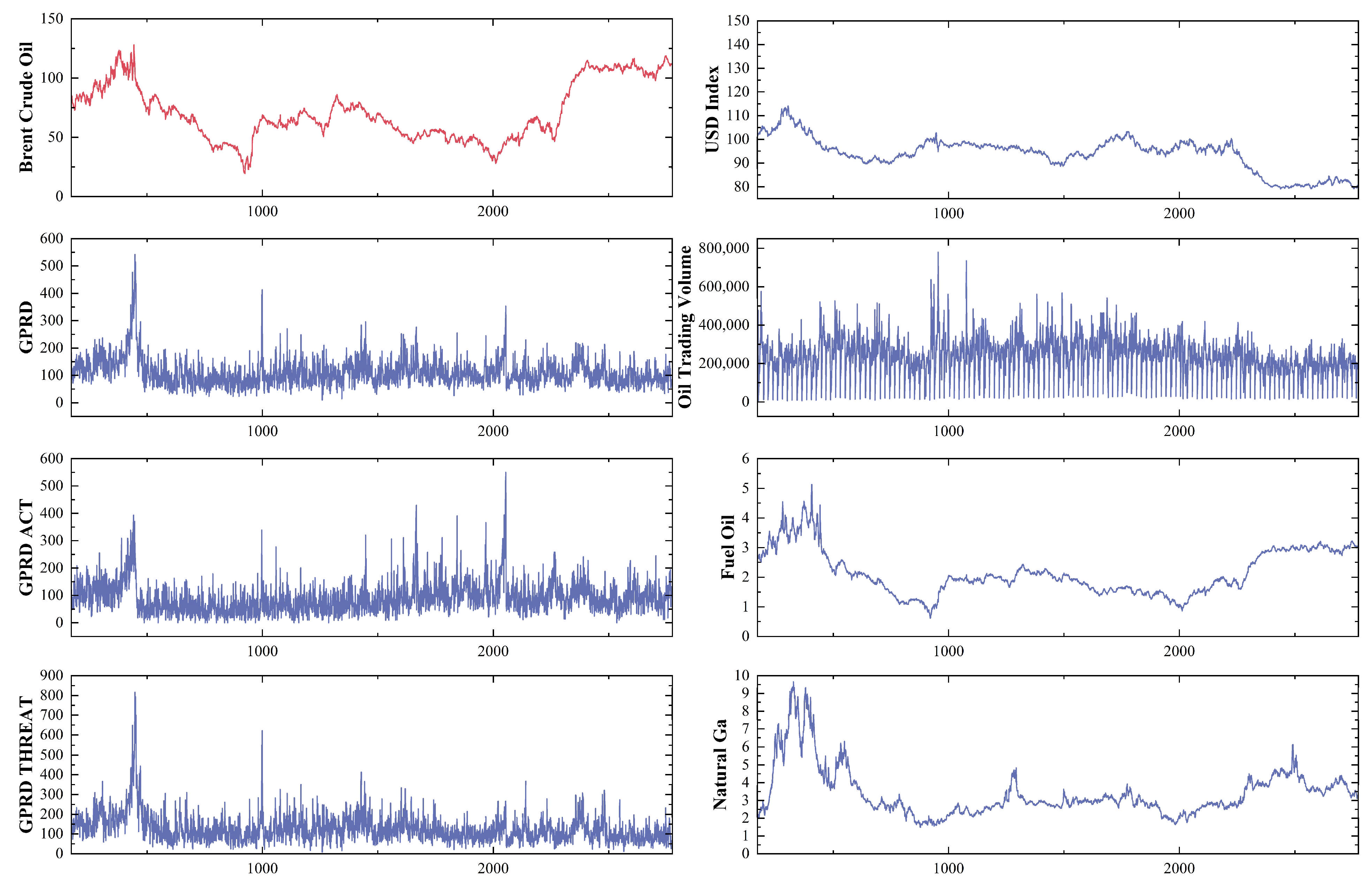
All of the above influences are chosen to coincide with the time period of the oil price, as shown in Figure 4.

4.2. Evaluation Principles

To measure the prediction performance of the prediction model, four evaluation indicators, including the Mean Absolute Error (MAE), Root Mean Square Error (RMSE), Mean Absolute Percentage Error (MAPE), coefficient of determination (R²), index of agreement (IA), and Theil U statistic 1 (U1), are selected in this study to verify the prediction accuracy of the proposed model. The equations are as follows:

$$MAE=T^{-1}{\sum }_{t=1}^T\left|Y_{(t)}-{\widehat{Y}}_{(t)}\right|$$

(39)

$$RMSE=(T^{-1}{\sum }_{t=1}^T(Y_{(t)}-{\widehat{Y}}_{(t)}{)}^2{)}^2$$

(40)

$$MAPE=T^{-1}{\sum }_{t=1}^T{\displaystyle \frac{\mid {\mathit{Y}}_{(t)}-{\widehat{\mathit{Y}}}_{(t)}\mid }{{\mathit{Y}}_{(t)}}}$$

(41)

$$R^2={\displaystyle \frac{{\sum }_{t=1}^T({\widehat{Y}}_{(t)}-\overline{Y}{)}^2}{{\sum }_{t=1}^T(Y_{(t)}-\overline{Y}{)}^2}}$$

(42)

$$IA=1-{\displaystyle \frac{{{\sum }_{t=1}^T\left(Y_{(t)}-{\widehat{Y}}_{(t)}\right)}^2}{{{\sum }_{t=1}^T\left(\left|{\widehat{Y}}_{(t)}-\hat{Y}\right|+\left|Y_{(t)}-\hat{Y}\right|\right)}^2}}$$

(43)

$$U1=(T^{-1}{\displaystyle \frac{{\sum }_{t=1}^T(Y_{(t)}-{\widehat{Y}}_{(t)}{)}^2}{\sqrt{T^{-1}{\sum }_{t=1}^T{Y}_{(t)}^2}+\sqrt{T^{-1}{{\sum }_{t=1}^T\widehat{Y}}_{(t)}^2}}}{)}^{{\displaystyle \frac{1}{2}}}$$

(44)

where $Y_{(t)}$ is the true value at time t, ${\widehat{Y}}_{(t)}$ is the predicted value at time t, $\overline{Y}$ is the mean of the predicted values, $\hat{Y}$ is the mean of the true values, and $T$ is the sample size. The MAE, RMSE, and MAPE reveal the differences between the true and predicted values, and R² reflects the proportion of the total variation in the dependent variable that can be explained based on the independent variable through a regression relationship. The IA value is used to reflect the generalization ability of the model, and the U1 is used to evaluate the prediction ability. The closer its value is to 0, the better the prediction ability of the prediction model.

4.3. Parameter Description

In this study, ICEEMDAN is used to decompose the oil price. BOHB is also employed to optimize the LSTM model.

The model parameters are selected as indicated in

Table 1. Model parameter settings.

Model	Parameters
ICEEMDAN	Noise standard deviation 0.2 Number of realizations 500 Maximum number of sifting iterations 5000

. The ICEEMDAN parameters are set as follows: the signal-to-noise ratio of the added white noise is 0.2, the number of noise additions is 500, and the maximum iteration number is 5000.

The hyperparameters in LSTM are optimized using BOHB. The hyperparameters chosen for this study included batch size, number of hidden layers, learning rate, and optimization range, as shown in

Table 2. Optimized settings for hyperparameters.

Hyperparameters	Range
Batch size	[32, 1024]
Number of hidden layers	[50, 200]
Learning rate	[0.001, 0.0005]

.

4.4. Benchmarking Model

The benchmark comparison models used in this study are XGboost, XGBOOST (with influencing factors), LSTM, LSTM (with influencing factors), Attention-LSTM, BOHB-Attention-LSTM, ACBFS-BOHB-Attention-LSTM, ACBFS-BOHB-EEMD-Attention-LSTM, ACBFS-BOHB-CEEMDAN-Attention-LSTM, ACBFS-BOHB-ICEEMDAN-Attention-LSTM, and ACBFS-BOHB-ICEEMDAN-Attention-(XGBoost-LSTM), which are the 11 benchmark comparison models. Experiment 1: The XGBoost and LSTM models, as the benchmark models, are selected as comparison models for their wide application and good performance in the field of machine learning, and this experiment is comnducted in order to validate the effects on the prediction model of the introduction of the influencing factors. Experiment 2: Attention mechanisms are used as comparative models to explore their effects on the prediction model. Experiment 3: Further comparison of different decomposition algorithms, including EEMD, CEEMDAN, ICEEMDAN. These decomposition algorithms help to better capture the trend and periodicity of the price. Experiment 4: Based on Experiment 3, LSTM and XGBoost are combined to form a hybrid LSTM-XGBoost model. The purpose of this model is to take full advantage of LSTM’s strength in capturing smooth features and XGBoost’s strong performance in integrating high-frequency features. Experiment 5: Based on Experiment 4, error correction is introduced by using the XGBoost model to predict the error sequence and correct the predictions of the previous model.

The relative performance and advantages of the proposed models in crude oil price forecasting can be evaluated by comparing them with benchmark models. The comparison of these models can assist in understanding the applicability and limitations of different methods and provide guidance for further research and application. The experimental results are detailed in Section 5.

5. Empirical Results

5.1. Comparison I

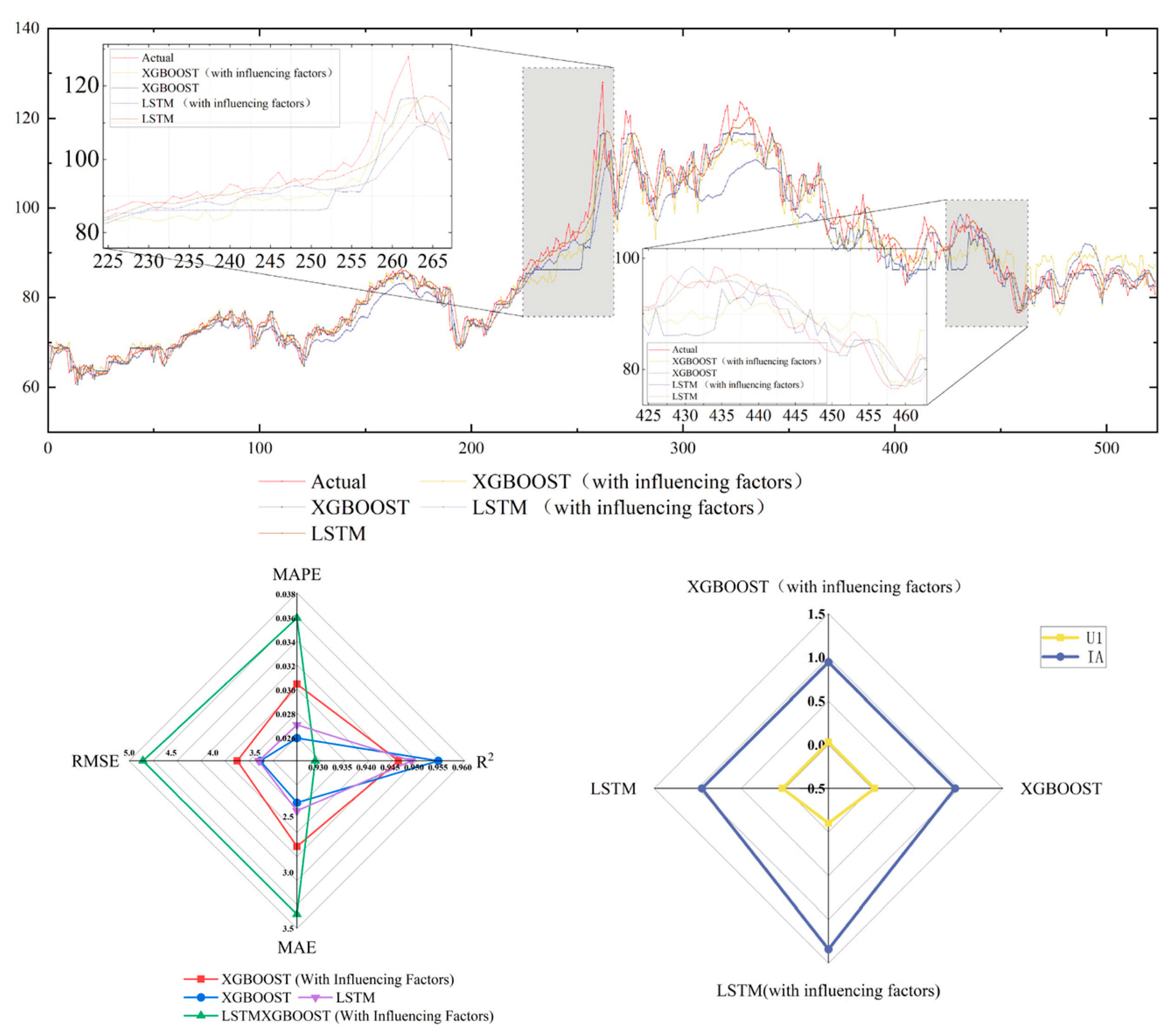
As shown in Figure 5, notable differences are observed in the performance of the various oil price prediction models. Contrary to expectations, the XGBoost model incorporating influential variables does not yield superior accuracy. Instead, the model excluding these variables consistently outperforms its counterpart across most evaluation metrics, including the MAE, RMSE, R², and MAPE. A similar pattern is evident in the LSTM models, where the exclusion of influential variables also results in improved predictive accuracy. These findings suggest that the inclusion of such factors does not necessarily enhance model performance in this context, and may, in fact, introduce unnecessary noise.

As shown in

Table 3. Comparison II model evaluation indicator results.

Evaluation Indicators	XGBOOST (With Influencing Factors)	XGBOOST	LSTM (With Influencing Factors)	LSTM
MAE	2.7679	2.3740	3.3734	2.4492
RMSE	3.7108	3.4370	4.8361	3.4531
R2	94.62%	95.45%	92.88%	94.89%
MAPE	3.04%	2.59%	3.59%	2.70%
IA	0.9436	0.9517	0.9042	0.9514
U1	0.0299	0.0277	0.0393	0.0277

, the XGBoost model exhibits strong performance in terms of the IA and U1, with values of 0.9517 and 0.0277, respectively. These results indicate a close alignment between the model’s predictions and actual observations, alongside minimal forecasting error.

In summary, a careful re-evaluation of the results reveals a key finding: contrary to initial expectations, the inclusion of influential factors did not enhance model accuracy. Instead, both the XGBoost and LSTM models excluding these variables consistently outperformed their counterparts across all evaluation metrics, including the MAE, RMSE, R², MAPE, IA, and U1. This suggests that, in the context of this specific oil price prediction task, the incorporation of such factors may introduce noise, thereby reducing predictive performance. Further investigation is therefore warranted to better understand this outcome and to identify more suitable modelling approaches for improving forecast accuracy.

5.2. Comparison II

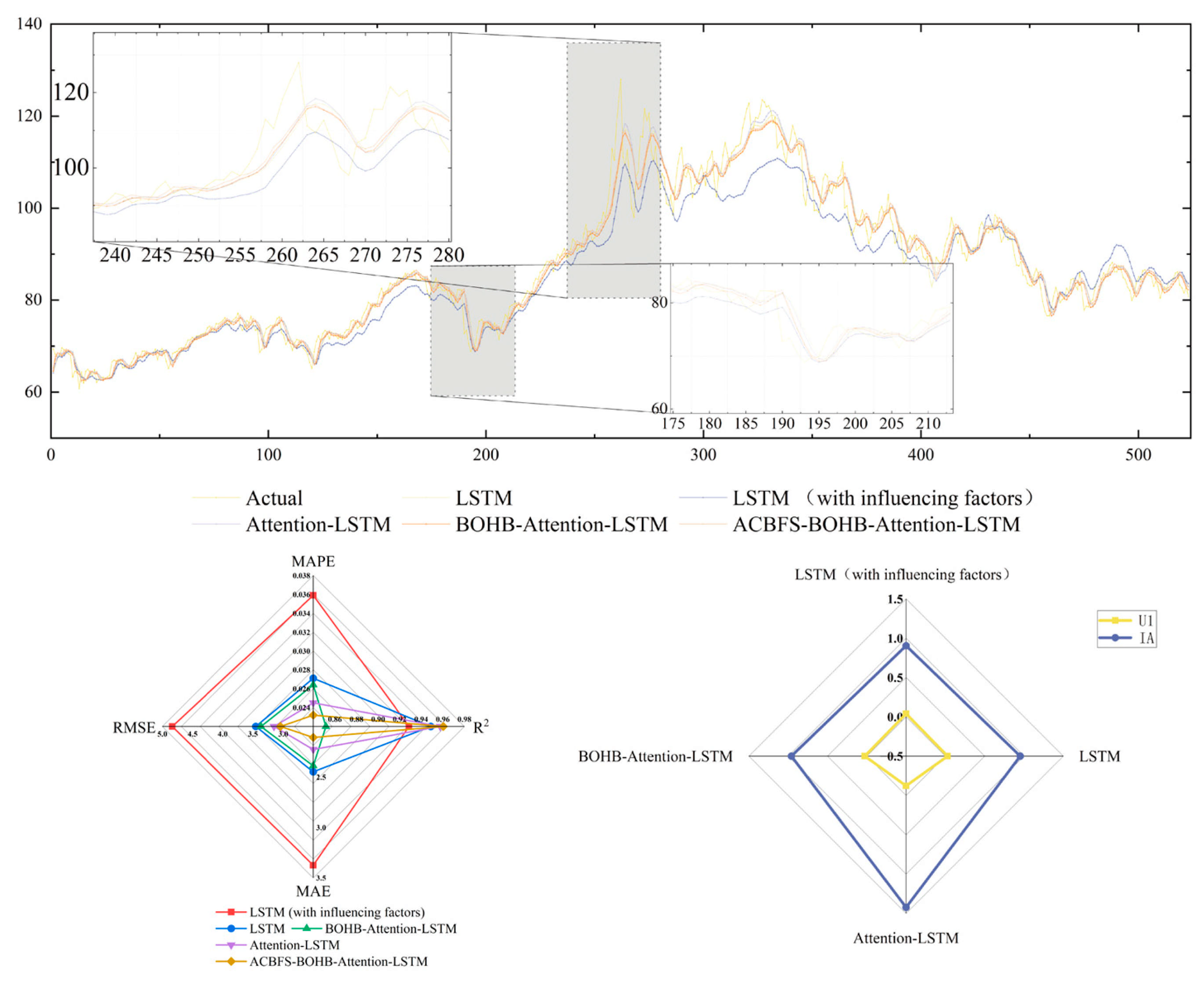
In light of the trajectory delineated by Comparison I, it is evident that although the LSTM model slightly underperforms compared to the XGBoost model on certain metrics, its predictive trend aligns more closely with the actual values. This suggests that the LSTM model may be better suited to capturing long-term patterns and the inherent volatility of oil price dynamics. Accordingly, Comparison II focuses on the LSTM model as a baseline, incorporating an attention mechanism and optimization algorithm to evaluate its forecasting performance. The models examined include LSTM (with influential factors), LSTM, Attention-LSTM, BOHB-Attention-LSTM, and ACBFS-BOHB-Attention-LSTM. As shown in Figure 6, the predictive results of these models are compared.

An initial comparative evaluation is conducted of the LSTM models with and without influential factors. The results indicate that the LSTM model without influential factors performs better across several evaluation metrics, exhibiting the MAE and RMSE, along with a higher R².

Subsequently, LSTM models enhanced by the incorporation of the attention mechanism were evaluated. The results clearly demonstrate that the Attention-LSTM model outperforms its counterparts across multiple metrics, with a lower MAE, RMSE, and MAPE, and a higher IA. This highlights the attention mechanism’s ability to improve the model’s focus on critical elements within the input sequence, thereby enhancing predictive accuracy. By dynamically adjusting the weights assigned to different segments of the sequence, the mechanism enables the model to prioritize the inputs most relevant to the prediction target, reducing the impact of irrelevant or noisy data. When applied to LSTM models that include influential factors, the attention mechanism further strengthens the model’s ability to identify and utilize variables with greater predictive relevance, thereby improving forecasting performance.

Moreover, the performance of the Attention-LSTM model is further enhanced through the integration of optimization algorithms, namely BOHB and ACBFS. The empirical results indicate that the BOHB-Attention-LSTM model achieves incremental improvements across multiple metrics, including reductions in the MAE, RMSE, and MAPE, along with an increase in the IA. Ultimately, the ACBFS-BOHB-Attention-LSTM model demonstrates the strongest overall performance, yielding the lowest MAE, RMSE, MAPE, and U1 values, and the highest R² and IA scores, as detailed in

Table 4. Comparison II evaluation indicator results.

Evaluation Indicators	LSTM (With Influencing Factors)	LSTM	Attention-LSTM	BOHB-Attention-LSTM	ACBFS-BOHB-Attention-LSTM
MAE	3.3734	2.4492	2.3904	2.2277	2.1082
RMSE	4.8361	3.4531	3.3681	3.1534	3.0459
R2	92.88%	94.89%	85.17%	95.76%	96.05%
MAPE	3.59%	2.71%	2.64%	2.45%	2.32%
IA	0.9042	0.9514	0.9538	0.9595	0.9622
U1	0.0393	0.0277	0.0270	0.0253	0.0244

. These findings clearly highlight the superiority of the ACBFS-BOHB-Attention-LSTM model in terms of predictive accuracy and the effective mitigation of error propagation in oil price forecasting.

Finally, a progressive enhancement trajectory is observed with the refinement of the Attention-LSTM model through the integration of optimization algorithms such as BOHB and ACBFS. The empirical results confirm the incremental improvements achieved by the BOHB-Attention-LSTM model, reflected by the lower MAE, RMSE, and MAPE values, as well as an increase in the IA. The optimal performance is ultimately attained by the ACBFS-BOHB-Attention-LSTM model, which records the lowest MAE, RMSE, MAPE, and U1, along with the highest R² and IA, thereby reaffirming its superiority in predictive accuracy and error reduction within the context of oil price forecasting.

5.3. Comparison III

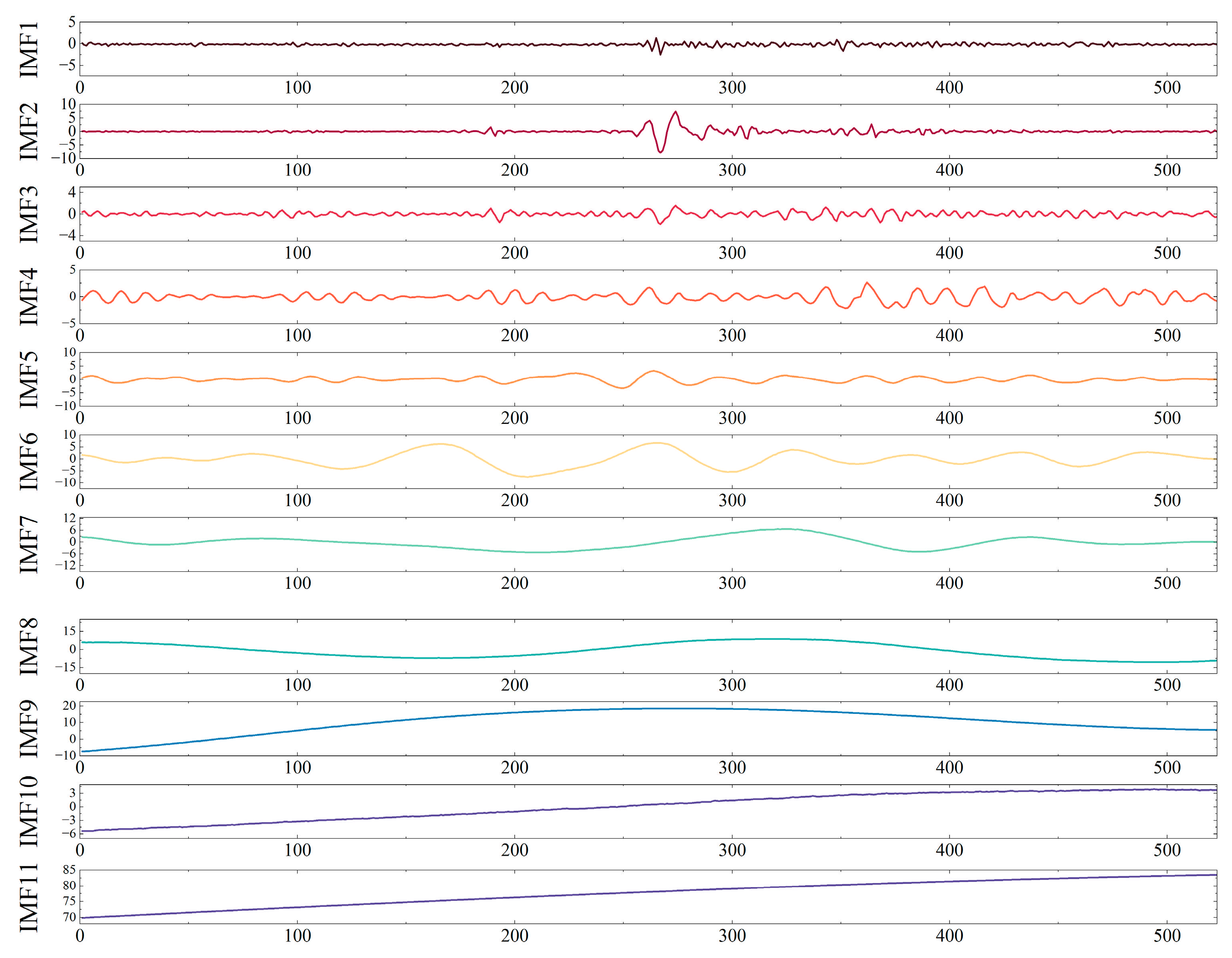
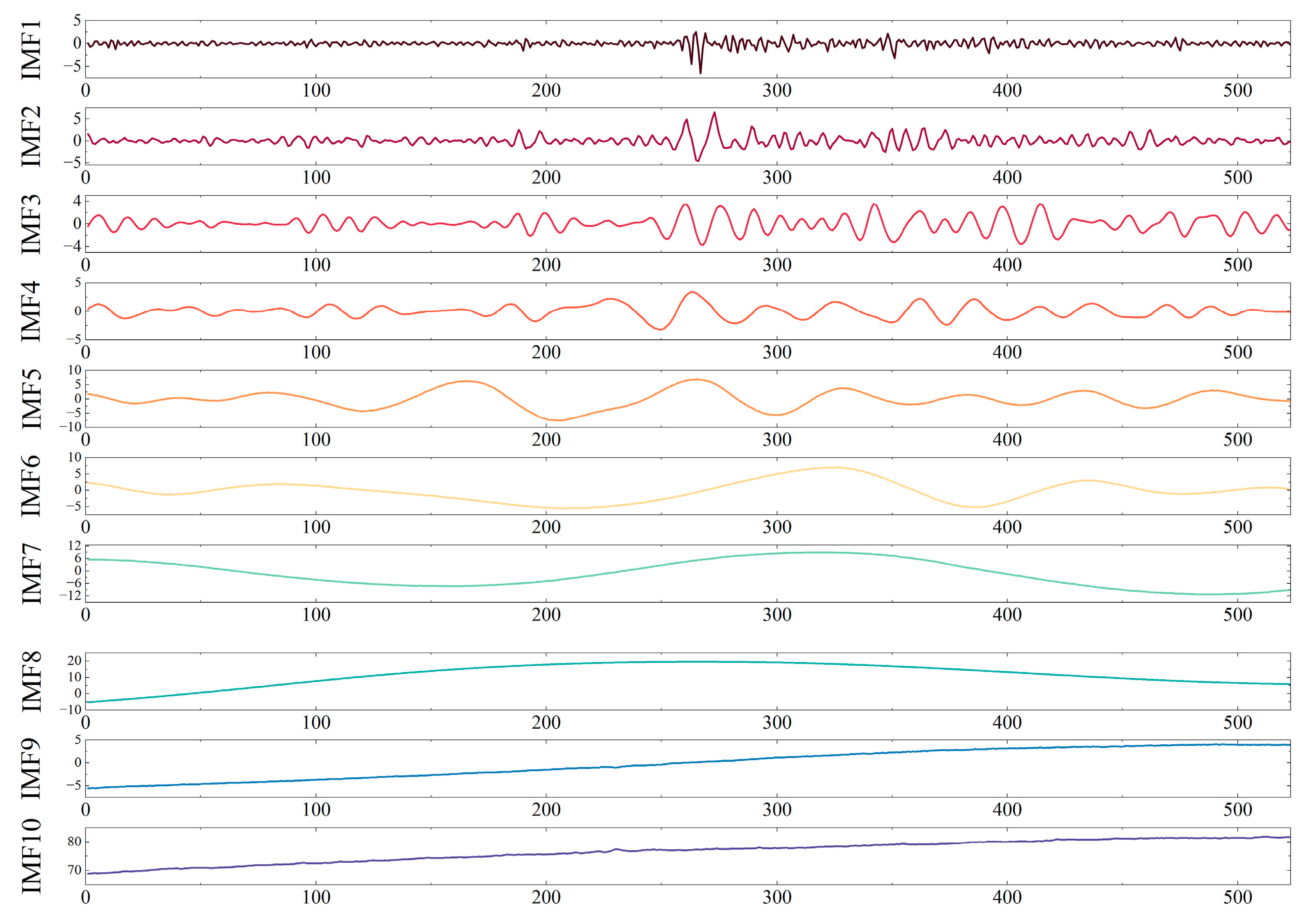
To improve the extraction and utilization of latent patterns and trends, Comparison III introduces a signal decomposition algorithm into the ACBFS-BOHB-Attention-LSTM model. The raw data are decomposed into multiple subsequences, each representing distinct patterns across various temporal scales. By modelling each timescale individually, predictive accuracy is enhanced. This integration increases the model’s adaptability and robustness, enabling the more effective capture of dynamic fluctuations within the data. The decomposition results of different decomposition methods are shown in Figure 7, Figure 8 and Figure 9.

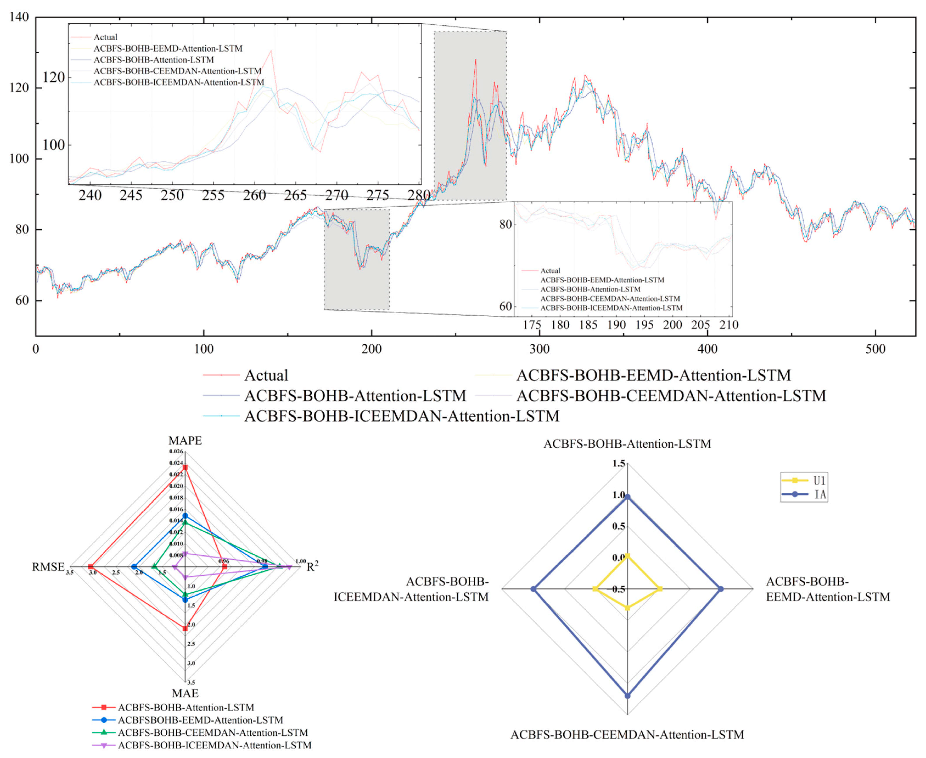
By observing Figure 6, it becomes apparent that the ACBFS-BOHB-Attention-LSTM model demonstrates commendable performance in the prediction of oil price. Nonetheless, the predictive prowess of the model experiences a significant enhancement upon the integration of diverse decomposition algorithms, as depicted in Figure 10.

Primarily, with respect to accuracy and precision metrics, the inclusion of the decomposition algorithm significantly enhances model performance. For the MAPE, all models in Comparison Ⅲ exhibit minimal error percentages, indicating their effectiveness in accurately predicting oil price trends. Notably, the ACBFS-BOHB-ICEEMDAN-Attention-LSTM model achieves a MAPE of 0.83%, reflecting a substantial reduction in error compared to alternative models. Similarly, in terms of the RMSE and MAE, this model attains the lowest error values of 1.2258 and 0.7699, respectively. In addition, the R² metric assesses the models’ ability to explain variability in the target variable. As shown in

Table 5. Comparison III evaluation indicator results.

Evaluation Indicators	ACBFS-BOHB-Attention-LSTM	ACBFSBOHB-EEMD-Attention-LSTM	ACBFS-BOHB-CEEMDAN-Attention-LSTM	ACBFS-BOHB-ICEEMDAN-Attention-LSTM
MAE	2.1082	1.3567	1.2256	0.7699
RMSE	3.0459	2.1057	1.6666	1.2258
R2	96.05%	98.16%	98.91%	99.41%
MAPE	2.32%	1.48%	1.36%	0.83%
IA	0.9622	0.9819	0.9887	0.9939
U1	0.0244	0.0169	0.0134	0.0098

, all models demonstrate strong R² scores, indicating their proficiency in capturing fluctuations in oil prices. The ACBFS-BOHB-ICEEMDAN-Attention-LSTM model achieves an R² of 99.41%, highlighting its superior performance in fitting training data and making precise predictions. Regarding the U1 metric, the ACBFS-BOHB-ICEEMDAN-Attention-LSTM model outperforms others with a score of 0.0098, representing a reduction of approximately 0.0146 compared to the ACBFS-BOHB-Attention-LSTM model’s score of 0.0244. Furthermore, the ACBFS-BOHB-ICEEMDAN-Attention-LSTM model achieves an IA score of 0.9939, marking an improvement of roughly 0.0317 compared the ACBFS-BOHB-Attention-LSTM model’s score of 0.9622. This underscores that the integration of the decomposition model enhances the model’s ability to adapt to predictive error distributions, improving its stability and reliability.

In conclusion, this section focuses on the enhancement of the ACBFS-BOHB-Attention-LSTM model through the integration of various decomposition algorithms, resulting in significant performance improvements. The ACBFS-BOHB-ICEEMDAN-Attention-LSTM model demonstrates strong performance across multiple evaluation metrics, including the MAPE, RMSE, MAE, R², U1, and IA. This highlights that the incorporation of a decomposition algorithm improves the accuracy, stability, and reliability of the oil price forecasting model, enabling a better explanation of the target variable variability and refinement of predictive error distributions.

5.4. Comparison IV

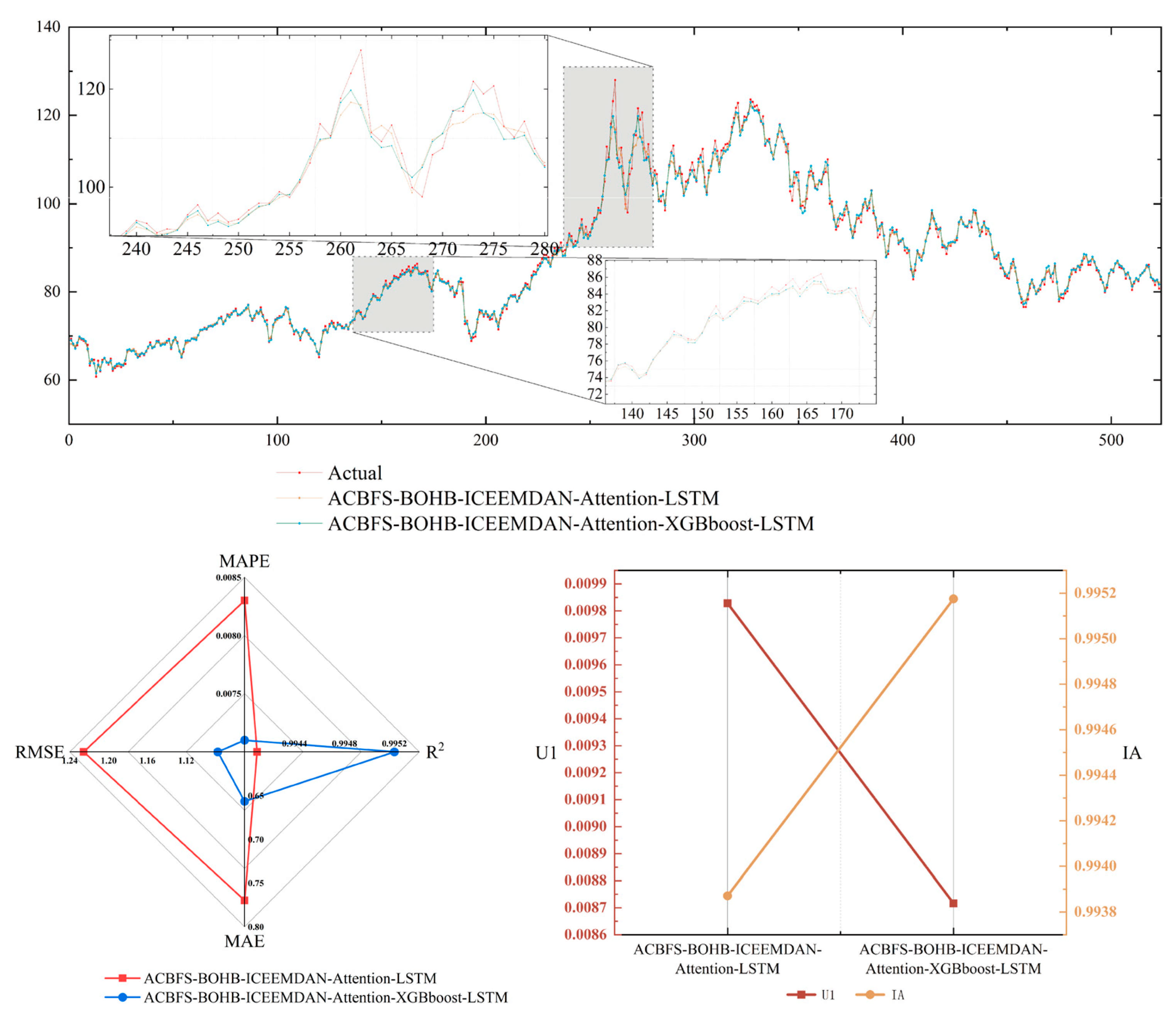
The findings from Comparison I highlight the exceptional accuracy and robust performance of the XGBoost model in oil price prediction. Building on these promising results, Comparison IV is conducted with the aim of leveraging the strengths of both the LSTM and XGBoost models through their integration into a hybrid LSTM-XGBoost model. In this framework, the LSTM model is used to predict the low-frequency component, while the XGBoost model handled the high-frequency component. Comparison IV is designed to explore the inherent advantages of the ACBFS-BOHB-ICEEMDAN-Attention-LSTM-XGBoost hybrid model and assess its effectiveness in oil price forecasting.

Table 6. ACBFS calculates lag step results.

imf1	imf2	imf3	imf4	imf5	imf6	imf7	imf8	imf9	imf10
1	1	1	1	1	1	1	1	1	1
2	2	2	2	2	2	2	2	2	2
	3	3	3	3	3	3
	4	7	6	5	4	4
	8		15	7	7	14
				11	10	18
				17	14
					20

presents the results of the lag step calculation for IMFs obtained through the ACBFS. According to Figure 11, the predictive results of the ACBFS-BOHB-ICEEMDAN-Attention-XGBoost-LSTM model demonstrate a thorough understanding of the oil price trend, especially during periods of significant price fluctuations. A detailed examination of the graphical representation in Figure 11, alongside the results in

Table 7. Comparison IV evaluation indicator results.

Evaluation Indicators	ACBFS-BOHB-ICEEMDAN-Attention-LSTM	ACBFS-BOHB-ICEEMDAN-Attention-XGBboost-LSTM
MAE	0.7699	0.6566
RMSE	1.2258	1.0876
R2	99.41%	99.52%
MAPE	0.83%	0.71%
IA	0.9939	0.9952
U1	0.0098	0.0087

, reveals that the ACBFS-BOHB-ICEEMDAN-Attention-XGBoost-LSTM hybrid model consistently outperforms all the other models across all evaluation metrics. Specifically, the hybrid model achieves lower values for the MAE, RMSE, and MAPE, indicating reduced prediction discrepancies. Additionally, improvements in the R² value, along with enhanced IA and U1 metrics, collectively demonstrate the model’s superior accuracy and predictive performance.

5.5. Comparison V

In Comparison V, building upon the previously established model (ACBFS-ICEEMDAN-BOHB-(XGBoost-LSTM)), an error correction mechanism is introduced to enhance oil price prediction accuracy. The rationale for incorporating this mechanism lies in its ability to capture and correct deviations and discrepancies in the model’s predictions. This approach aims to improve model stability and precision, thereby increasing its adaptability to complex fluctuations in oil price dynamics and providing more reliable forecasts.

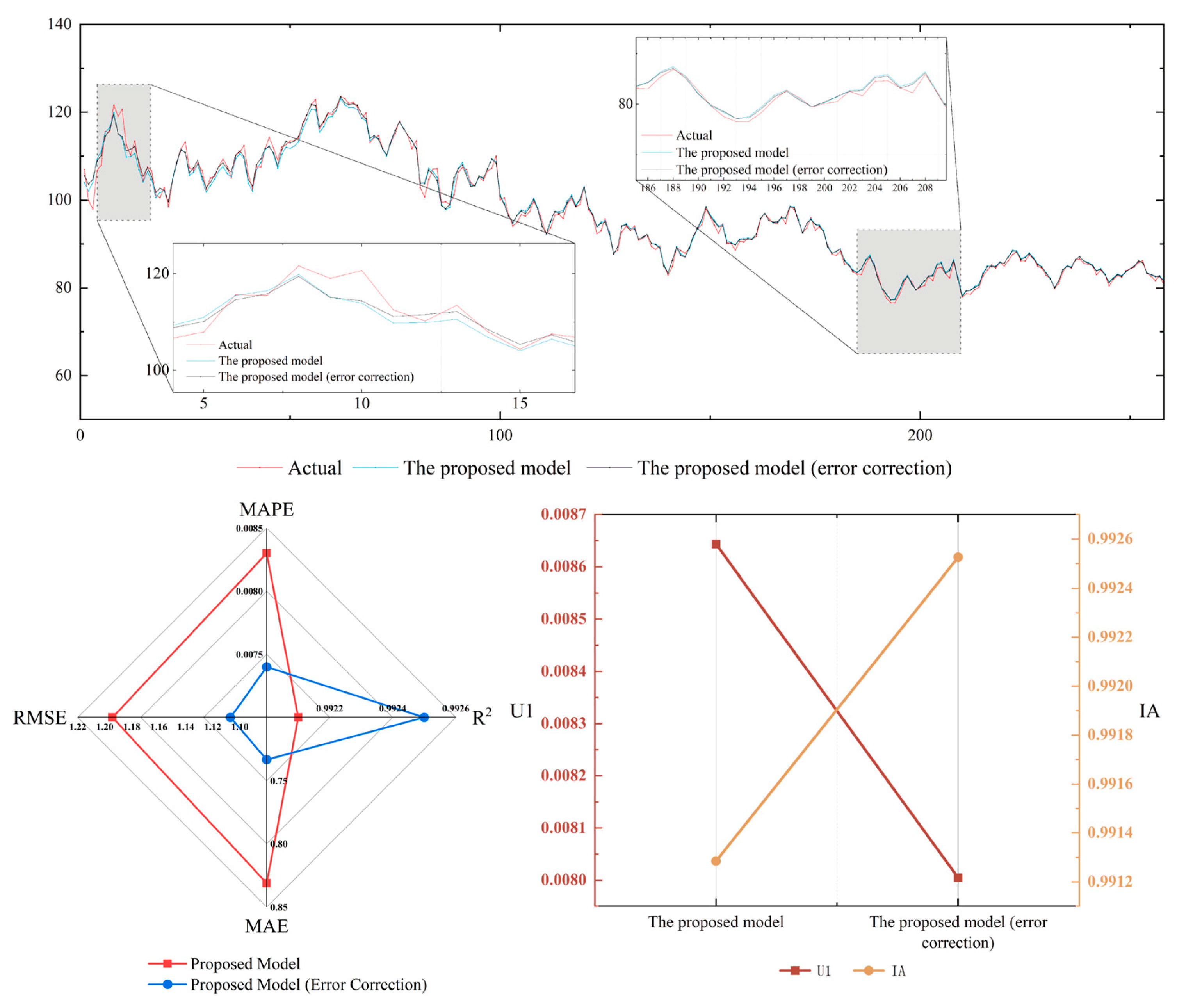
The core function of this mechanism is to rectify the model’s predictions through error sequence forecasting, thereby enhancing prediction accuracy. Specifically, the initial ACBFS-ICEEMDAN-BOHB-(XGBoost-LSTM) model is used to predict oil prices, generating preliminary forecasts. These forecasts are then compared with actual observations, enabling the computation of an error series. The XGBoost model is subsequently employed to predict the error sequence, providing forecasts for the errors. These predicted errors are then used to adjust the initial model’s predictions by incorporating or subtracting the error values. Through this iterative process, the predicted errors are effectively used to reduce model deviations, resulting in improved prediction accuracy.

As shown in Figure 12 and

Table 8. Comparison V evaluation indicator results.

Evaluation Indicators	Proposed Model	Proposed Model (Error Correction)
MAE	0.8311	0.7333
RMSE	1.1944	1.1069
R2	99.21%	99.25%
MAPE	0.83%	0.74%
IA	0.9913	0.9925
U1	0.0086	0.0080

, the model incorporating the error correction mechanism outperforms the original model across multiple metrics. Specifically, the error-corrected model achieves MAE, RMSE, and MAPE values of 0.7333, 1.1069, and 0.7413%, respectively, demonstrating a significant improvement on the results obtained using the standalone model. Furthermore, the R² coefficient shows notable enhancement, reaching 99.25%, indicating the error-corrected model’s improved ability to explain variance in the target variable.

In terms of the IA and U1 metrics, the error-corrected model also performs favourably. The IA value of 0.9925 reflects enhanced model consistency, while the U1 value decreases to 0.0080, suggesting an improved capacity to accommodate anomalies and outliers. In conclusion, the integration of the error correction mechanism leads to a substantial improvement in the oil price prediction model’s effectiveness. By leveraging the error series predictions, this mechanism refines the model’s forecasts, resulting in increased precision and reliability in the final predictions.

6. Conclusions

The primary objective of this research is to develop an innovative framework for forecasting crude oil prices, addressing the complex forecasting challenges inherent to the crude oil market. The framework combines multidimensional feature selection algorithms, signal decomposition techniques, and hybrid models, and the validity of the proposed framework is confirmed by comparing several benchmark models. The main conclusions obtained from this study are as follows:

(1) The incorporation of multidimensional influences is uncertain in terms of improvement in prediction accuracy. The experimental results of this study verified that simply incorporating all the influencing factors into XGBoost or LSTM does not improve the prediction accuracy, but rather leads to a loss of accuracy due to overfitting. The introduction of ACBFS to select key features can significantly improve the prediction accuracy, which fully demonstrates that feature engineering is essential to avoid the inclusion of redundant information;

(2) Efficacy of Signal Decomposition Techniques: In the data preprocessing stage, the application of signal decomposition techniques introduces an essential enhancement to the proposed forecasting framework. Methods such as EEMD, CEEMDAN, and ICEEMDAN enable the separation of high- and low-frequency components from raw data, yielding a more precise representation of underlying trends and periodic patterns. ICEEMDAN has the best decomposition, with 42.35% and 37.18% improvements in the MAE compared to EEMD and CEEMDAN;

(3) Benefits of Hybrid Models: The framework proposed in this study combines the Attention Mechanism, LSTM, and XGBoost, exploiting the advantages of each of these methods for modelling different volatility characteristics. The empirical results demonstrate the ability of the hybrid model to capture complex patterns of price fluctuations and substantially improve forecasting accuracy. Compared to AM-LSTM alone, the combination of XGBoost improved the MAE, RMSE, R², MAPE, IA, and U1 by 14.72%, 11.27%, 0.11%, 14.46%, 0.13%, and 11.22%, respectively. This emphasizes the value of hybrid models and maps out possible prospects for future research efforts addressing similar challenges;

(4) Efficacy of Error Correction Mechanism: This study introduces an error correction mechanism into the framework, which aims to predict the residual sequences and correct the predictions using the XGBoost model. The empirical assessment shows that the mechanism performs satisfactorily, which strengthens the robustness and reliability of the framework; the MAE decreased from 0.8311 to 0.7333. The error correction mechanism not only improves the prediction accuracy, but also enables the model to adaptively adapt to market fluctuations.

Overall, the hybrid framework proposed in this study demonstrates strong competitiveness in oil price forecasting. However, there is still room for improvement in feature engineering and decomposition method improvement. First, this study incorporates many structured features; however, unstructured features such as investor sentiment can be further considered in future research. Second, although the decomposition method substantially improves the model accuracy, there are still challenges in real-time decomposition and prediction, and how to build a real-time prediction system is still a research priority in the future.

References

1. Statistical Review of World Energy 2022. 2022. Available online: https://www.bp.com/content/dam/bp/business-sites/en/global/corporate/pdfs/energy-economics/statistical-review/bp-stats-review-2022-full-report.pdf (accessed on 7 May 2020).
2. Xie, H.; Khurshid, A.; Rauf, A.; Khan, K.; Calin, A.C. Is Geopolitical Turmoil Driving Petroleum Prices and Financial Liquidity Relationship? Wavelet-Based Evidence from Middle-East. Def. Peace Econ. 2022, 34, 810–826. [Google Scholar] [CrossRef]
3. Wu, C.; Wang, J.; Hao, Y. Deterministic and Uncertainty Crude Oil Price Forecasting Based on Outlier Detection and Modified Multi-Objective Optimization Algorithm. Resour. Policy 2022, 77, 102780. [Google Scholar] [CrossRef]
4. Kisswani, K.M.; Nusair, S.A. Non-Linearities in the Dynamics of Oil Prices. Energy Econ. 2013, 36, 341–353. [Google Scholar] [CrossRef]
5. Adekoya, O.B.; Asl, M.G.; Oliyide, J.A.; Izadi, P. Multifractality and Cross-Correlation between the Crude Oil and the European and Non-European Stock Markets during the Russia-Ukraine War. Resour. Policy 2023, 80, 103134. [Google Scholar] [CrossRef]
6. Ahmed, S.; Alshater, M.M.; Ammari, A.E.; Hammami, H. Artificial Intelligence and Machine Learning in Finance: A Bibliometric Review. Res. Int. Bus. Financ. 2022, 61, 101646. [Google Scholar] [CrossRef]
7. Jammazi, R.; Aloui, C. Crude Oil Price Forecasting: Experimental Evidence from Wavelet Decomposition and Neural Network Modeling. Energy Econ. 2012, 34, 828–841. [Google Scholar] [CrossRef]
8. Henderson, P.; Islam, R.; Bachman, P.; Pineau, J.; Precup, D.; Meger, D. Deep Reinforcement Learning That Matters; Springer: Singapore, 2019. [Google Scholar]
9. Yahya, M.; Kanjilal, K.; Dutta, A.; Uddin, G.S.; Ghosh, S. Can Clean Energy Stock Price Rule Oil Price? New Evidences from a Regime-Switching Model at First and Second Moments. Energy Econ. 2021, 95, 105116. [Google Scholar] [CrossRef]
10. Nomikos, N.; Andriosopoulos, K. Modelling Energy Spot Prices: Empirical Evidence from NYMEX. Energy Econ. 2012, 34, 1153–1169. [Google Scholar] [CrossRef]
11. Dash, D.P.; Sethi, N.; Bal, D.P. Is the Demand for Crude Oil Inelastic for India? Evidence from Structural VAR Analysis. Energy Policy 2018, 118, 552–558. [Google Scholar] [CrossRef]
12. Niu, X.; Wang, J.; Zhang, L. Carbon Price Forecasting System Based on Error Correction and Divide-Conquer Strategies. Appl. Soft Comput. 2022, 118, 107935. [Google Scholar] [CrossRef]
13. Huang, L.; Wang, J. Global Crude Oil Price Prediction and Synchronization Based Accuracy Evaluation Using Random Wavelet Neural Network. Energy 2018, 151, 875–888. [Google Scholar] [CrossRef]
14. Fan, L.; Pan, S.; Li, Z.; Li, H. An ICA-Based Support Vector Regression Scheme for Forecasting Crude Oil Prices. Technol. Forecast. Soc. Change 2016, 112, 245–253. [Google Scholar] [CrossRef]
15. Chen, Y.; He, K.; Tso, G.K.F. Forecasting Crude Oil Prices: A Deep Learning Based Model. Procedia Comput. Sci. 2017, 122, 300–307. [Google Scholar] [CrossRef]
16. Niu, X.; Wang, J. A Combined Model Based on Data Preprocessing Strategy and Multi-Objective Optimization Algorithm for Short-Term Wind Speed Forecasting. Appl. Energy 2019, 241, 519–539. [Google Scholar] [CrossRef]
17. Askarzadeh, A. Comparison of Particle Swarm Optimization and Other Metaheuristics on Electricity Demand Estimation: A Case Study of Iran. Energy 2014, 72, 484–491. [Google Scholar] [CrossRef]
18. Falkner, S.; Klein, A.; Hutter, F. BOHB: Robust and Efficient Hyperparameter Optimization at Scale. In Proceedings of the International Conference on Machine Learning PMLR, Stockholm, Sweden, 10–15 July 2018; pp. 1437–1446. [Google Scholar]
19. Zhang, Y.; Liu, X.; Bao, F.; Chi, J.; Zhang, C.; Liu, P. Particle Swarm Optimization with Adaptive Learning Strategy. Knowl.-Based Syst. 2020, 196, 105789. [Google Scholar] [CrossRef]
20. Soleimanzade, M.A.; Sadrzadeh, M. Deep Learning-Based Energy Management of a Hybrid Photovoltaic-Reverse Osmosis-Pressure Retarded Osmosis System. Appl. Energy 2021, 293, 116959. [Google Scholar] [CrossRef]
21. Alameer, Z.; Fathalla, A.; Li, K.; Ye, H.; Jianhua, Z. Multistep-Ahead Forecasting of Coal Prices Using a Hybrid Deep Learning Model. Resour. Policy 2020, 65, 101588. [Google Scholar] [CrossRef]
22. Xie, Y.; Hu, P.; Zhu, N.; Lei, F.; Xing, L.; Xu, L.; Sun, Q. A Hybrid Short-Term Load Forecasting Model and Its Application in Ground Source Heat Pump with Cooling Storage System. Renew. Energy 2020, 161, 1244–1259. [Google Scholar] [CrossRef]
23. Ahmad, W.; Aamir, M.; Khalil, U.; Ishaq, M.; Iqbal, N.; Khan, M. A New Approach for Forecasting Crude Oil Prices Using Median Ensemble Empirical Mode Decomposition and Group Method of Data Handling. Math. Probl. Eng. 2021, 2021, e5589717. [Google Scholar] [CrossRef]
24. Jiang, H.; Hu, W.; Xiao, L.; Dong, Y. A Decomposition Ensemble Based Deep Learning Approach for Crude Oil Price Forecasting. Resour. Policy 2022, 78, 102855. [Google Scholar] [CrossRef]
25. Zhou, F.; Huang, Z.; Zhang, C. Carbon Price Forecasting Based on CEEMDAN and LSTM. Appl. Energy 2022, 311, 118601. [Google Scholar] [CrossRef]
26. Bedi, J.; Toshniwal, D. Empirical Mode Decomposition Based Deep Learning for Electricity Demand Forecasting. IEEE Access 2018, 6, 49144–49156. [Google Scholar] [CrossRef]
27. Wu, Y.-X.; Wu, Q.-B.; Zhu, J.-Q. Improved EEMD-Based Crude Oil Price Forecasting Using LSTM Networks. Phys. A Stat. Mech. Its Appl. 2019, 516, 114–124. [Google Scholar] [CrossRef]
28. Dolatnia, N.; Fern, A.; Fern, X. Bayesian Optimization with Resource Constraints and Production. Int. Conf. Autom. Plan. Sched. ICAPS 2016, 26, 115–123. [Google Scholar] [CrossRef]
29. Rardin, R.L.; Uzsoy, R. Experimental Evaluation of Heuristic Optimization Algorithms: A Tutorial. J. Heuristics 2001, 7, 261–304. [Google Scholar] [CrossRef]
30. Feng, S.-W.; Chai, K. An Improved Method for EMD Modal Aliasing Effect. Vibroeng. Proced. 2020, 35, 76–81. [Google Scholar] [CrossRef]
31. Wen, J.; Zhao, X.-X.; Chang, C.-P. The Impact of Extreme Events on Energy Price Risk. Energy Econ. 2021, 99, 105308. [Google Scholar] [CrossRef]
32. Zhao, D.; Sibt e-Ali, M.; Omer Chaudhry, M.; Ayub, B.; Waqas, M.; Ullah, I. Modeling the Nexus between Geopolitical Risk, Oil Price Volatility and Renewable Energy Investment; Evidence from Chinese Listed Firms. Renew. Energy 2024, 225, 120309. [Google Scholar] [CrossRef]
33. Zhai, D.; Zhang, T.; Liang, G.; Liu, B. Research on Crude Oil Futures Price Prediction Methods: A Perspective Based on Quantum Deep Learning. Energy 2025, 320, 135080. [Google Scholar] [CrossRef]
34. Tao, Z.; Wang, M.; Liu, J.; Wang, P. A Functional Data Analysis Framework Incorporating Derivative Information and Mixed-Frequency Data for Predictive Modeling of Crude Oil Price. IEEE Trans. Ind. Inf. 2025, 21, 3226–3235. [Google Scholar] [CrossRef]
35. Montesinos López, O.A.; Montesinos López, A.; Crossa, J. Overfitting, Model Tuning, and Evaluation of Prediction Performance. In Multivariate Statistical Machine Learning Methods for Genomic Prediction; Springer International Publishing: Cham, Switzerland, 2022; pp. 109–139. ISBN 978-3-030-89009-4. [Google Scholar]
36. Benesty, J.; Chen, J.; Huang, Y.; Cohen, I. Pearson Correlation Coefficient. In Noise Reduction in Speech Processing; Springer Topics in Signal Processing; Springer: Berlin/Heidelberg, Germany, 2009; Volume 2, pp. 1–4. ISBN 978-3-642-00295-3. [Google Scholar]
37. Gierlichs, B.; Batina, L.; Tuyls, P.; Preneel, B. Mutual Information Analysis. In Cryptographic Hardware and Embedded Systems—CHES 2008; Oswald, E., Rohatgi, P., Eds.; Lecture Notes in Computer Science; Springer: Berlin/Heidelberg, Germany, 2008; Volume 5154, pp. 426–442. ISBN 978-3-540-85052-6. [Google Scholar]
38. Wang, Y.; Wang, Z.; Kang, X.; Luo, Y. A Novel Interpretable Model Ensemble Multivariate Fast Iterative Filtering and Temporal Fusion Transform for Carbon Price Forecasting. Energy Sci. Eng. 2023, 11, 1148–1179. [Google Scholar] [CrossRef]
39. Xiong, X.; Qing, G. A Hybrid Day-Ahead Electricity Price Forecasting Framework Based on Time Series. Energy 2023, 264, 126099. [Google Scholar] [CrossRef]
40. Xu, W.; Wang, Z.; Wang, W.; Zhao, J.; Wang, M.; Wang, Q. Short-Term Photovoltaic Output Prediction Based on Decomposition and Reconstruction and XGBoost under Two Base Learners. Energies 2024, 17, 906. [Google Scholar] [CrossRef]
41. Grinsztajn, L.; Oyallon, E.; Varoquaux, G. Why Do Tree-Based Models Still Outperform Deep Learning on Tabular Data? arXiv 2022, arXiv:2207.08815v1. [Google Scholar]
42. Vaswani, A.; Shazeer, N.; Parmar, N.; Uszkoreit, J.; Jones, L.; Gomez, A.N.; Kaiser, L.; Polosukhin, I. Attention Is All You Need. arXiv 2017, arXiv:1706.03762. [Google Scholar]
43. Zhang, G.P. Time Series Forecasting Using a Hybrid ARIMA and Neural Network Model. Neurocomputing 2003, 50, 159–175. [Google Scholar] [CrossRef]
44. Zheng, G.; Li, Y.; Xia, Y. Crude Oil Price Forecasting Model Based on Neural Networks and Error Correction. Appl. Sci. 2025, 15, 1055. [Google Scholar] [CrossRef]
45. Wang, Y.-H.; Yeh, C.-H.; Young, H.-W.V.; Hu, K.; Lo, M.-T. On the Computational Complexity of the Empirical Mode Decomposition Algorithm. Phys. A Stat. Mech. Its Appl. 2014, 400, 159–167. [Google Scholar] [CrossRef]
46. Wang, T.; Zhang, M.; Yu, Q.; Zhang, H. Comparing the Applications of EMD and EEMD on Time–Frequency Analysis of Seismic Signal. J. Appl. Geophys. 2012, 83, 29–34. [Google Scholar] [CrossRef]
47. Qin, Q.; He, H.; Li, L.; He, L.-Y. A Novel Decomposition-Ensemble Based Carbon Price Forecasting Model Integrated with Local Polynomial Prediction. Comput. Econ. 2020, 55, 1249–1273. [Google Scholar] [CrossRef]
48. Liu, H.; Mi, X.; Li, Y. Comparison of Two New Intelligent Wind Speed Forecasting Approaches Based on Wavelet Packet Decomposition, Complete Ensemble Empirical Mode Decomposition with Adaptive Noise and Artificial Neural Networks. Energy Convers. Manag. 2018, 155, 188–200. [Google Scholar] [CrossRef]
49. Ghimire, S.; Deo, R.C.; Casillas-Pérez, D.; Salcedo-Sanz, S. Improved Complete Ensemble Empirical Mode Decomposition with Adaptive Noise Deep Residual Model for Short-Term Multi-Step Solar Radiation Prediction. Renew. Energy 2022, 190, 408–424. [Google Scholar] [CrossRef]
50. Sklar, M. Fonctions de Répartition à n Dimensions et Leurs Marges. Ann. l’ISUP 1959, 8, 229–231. [Google Scholar]
51. Fleuret, F. Fast Binary Feature Selection with Conditional Mutual Information. J. Mach. Learn. Res. 2004, 5, 1531–1555. [Google Scholar]
52. Peng, L.; Wang, L.; Xia, D.; Dao, Q. Effective Energy Consumption Forecasting Using Empirical Wavelet Transform and Long Short-Term Memory. Energy 2022, 238, 121756. [Google Scholar] [CrossRef]
53. Florea, A.-C.; Andonie, R. Weighted Random Search for Hyperparameter Optimization. arXiv 2020, arXiv:2004.01628. [Google Scholar] [CrossRef]
54. Jiang, Z.; Zhao, L.; Li, S.; Jia, Y. Real-Time Object Detection Method Based on Improved YOLOv4-Tiny. arXiv 2020, arXiv:2011.04244. [Google Scholar]
55. Li, L.; Jamieson, K.; DeSalvo, G.; Rostamizadeh, A.; Talwalkar, A. Hyperband: A Novel Bandit-Based Approach to Hyperparameter Optimization. J. Mach. Learn. Res. 2017, 18, 6765–6816. [Google Scholar]
56. Bergstra, J.; Bardenet, R.; Bengio, Y.; Kégl, B. Algorithms for Hyper-Parameter Optimization. Adv. Neural Inf. Process. Syst. 2011, 24, 2546–2554. [Google Scholar]
57. Akhter, M.N.; Mekhilef, S.; Mokhlis, H.; Ali, R.; Usama, M.; Muhammad, M.A.; Khairuddin, A.S.M. A Hybrid Deep Learning Method for an Hour Ahead Power Output Forecasting of Three Different Photovoltaic Systems. Appl. Energy 2022, 307, 118185. [Google Scholar] [CrossRef]
58. Guliyev, H.; Mustafayev, E. Predicting the Changes in the WTI Crude Oil Price Dynamics Using Machine Learning Models. Resour. Policy 2022, 77, 102664. [Google Scholar] [CrossRef]
59. Abba Abdullahi, S.; Kouhy, R.; Muhammad, Z. Trading Volume and Return Relationship in the Crude Oil Futures Markets. Stud. Econ. Financ. 2014, 31, 426–438. [Google Scholar] [CrossRef]
60. Abiad, A.; Qureshi, I.A. The Macroeconomic Effects of Oil Price Uncertainty. Energy Econ. 2023, 125, 106839. [Google Scholar] [CrossRef]
61. Zhang, Z.; He, M.; Zhang, Y.; Wang, Y. Geopolitical Risk Trends and Crude Oil Price Predictability. Energy 2022, 258, 124824. [Google Scholar] [CrossRef]
62. Mensi, W.; Rehman, M.U.; Vo, X.V. Dynamic Frequency Relationships and Volatility Spillovers in Natural Gas, Crude Oil, Gas Oil, Gasoline, and Heating Oil Markets: Implications for Portfolio Management. Resour. Policy 2021, 73, 102172. [Google Scholar] [CrossRef]
63. Caldara, D.; Iacoviello, M. Measuring Geopolitical Risk. Am. Econ. Rev. 2022, 112, 1194–1225. [Google Scholar] [CrossRef]
Figure 1. The proposed hybrid model framework in this study.
Energies 18 02246 g001
Figure 2. LSTM cell structure.
Energies 18 02246 g002
Figure 3. Stacked learning.
Energies 18 02246 g003
Figure 4. Historical data on impact factors.
Energies 18 02246 g004
Figure 5. Comparison I forecast results.
Energies 18 02246 g005
Figure 6. Comparison II prediction results.
Energies 18 02246 g006
Figure 7. EEMD decomposition results.
Energies 18 02246 g007
Figure 8. CEEMDAN decomposition results.
Energies 18 02246 g008
Figure 9. ICEEMDAN decomposition results.
Energies 18 02246 g009
Figure 10. Comparison III prediction results.
Energies 18 02246 g010
Figure 11. Comparison IV prediction results.
Energies 18 02246 g011
Figure 12. Comparison V comparison chart of model prediction results.
Energies 18 02246 g012