Fault Diagnosis and Tolerant Control of Current Sensors Zero-Offset Fault in Multiphase Brushless DC Motors Utilizing Current Signals

Abstract

To address the issue of control inaccuracy caused by the zero-offset fault in current sensors within the multiphase brushless DC motor (BLDCM) drive system, this paper proposes a fault diagnosis and fault-tolerant control method based on current signals. Different from traditional solutions that rely on hardware redundancy or precise modeling, this method constructs a dual-channel fault diagnosis framework by integrating the steady-state amplitude offset of the phase current after the fault and the abnormal characteristics of dynamic sector switching. Firstly, sliding time window monitoring is used to identify steady-state amplitude anomalies and locate faulty sectors. Subsequently, an algorithm for detecting the difference in current changes during sector switching is designed, and a logic interlocking verification mechanism is combined to eliminate false triggering and accurately locate single or multiple fault phases. Furthermore, based on the diagnostic information, a repeated iterative online correction method is adopted to restore the accuracy of the current measurement. This method only relies on phase current signals and rotor position information, does not require additional hardware support or accurate system models, and is not affected by the nonlinear characteristics of the motor. Finally, the experimental verification was carried out on a nine-phase BLDCM drive system. Experimental results indicate that the torque fluctuation of the system can be controlled within 5% through the fault-tolerant control strategy.

1. Introduction

Multiphase motor drive systems have shown great potential in high-reliability application scenarios in the field of electric propulsion systems, such as aerospace systems, ship propulsion systems, electric vehicles, and high-power equipment due to their higher power density, lower torque fluctuation, and better fault tolerance [1,2,3,4,5]. Among them, multiphase BLDCM adopts a square wave drive strategy, and its control algorithm has certain advantages in torque fluctuation control and motor parameter accuracy to a certain extent [6]. Compared with systems that partially rely on sine wave control, its torque fluctuation rate after fault tolerance can be reduced to 3%, which is better than the 4.5% of the twelve-phase PMSM [7]. Secondly, BLDCM adopts a six-step or multi-step square wave control strategy, which does not rely on the analytical solution of the sinusoidal voltage trajectory, so the dependence on motor parameters such as stator inductance and phase resistance is significantly reduced, so it is suitable for scenarios with high performance output requirements [6,7].

However, the high-performance control of multiphase BLDCM relies on the accurate sampling of phase current by current sensors. However, in practical applications, current sensors are affected by working environments such as elevated temperature and moisture levels, which may cause sensor failure, thus causing misjudgment of the working status of the drive system [8,9]. In addition, owing to the expansion in phase count within multiphase motors, the demand for current sensors proportionally increases, which significantly increases the risk of failure and contributes to greater complexity in the system. Therefore, research on fault diagnosis and compensation strategy for multiphase BLDCM current sensors is of great significance.

Typical fault types in current sensors are wire break faults, gain faults, and zero-offset faults [10]. Among them, the zero-offset fault mode shows gradual changes and is difficult to detect immediately. Among them, the zero-offset fault mode shows gradual changes and is difficult to detect immediately. Compared with other fault modes, zero-offset faults are more likely to gradually appear under the influence of external factors such as long-term use or temperature changes, thus posing a huge challenge to accurate diagnosis [11,12]. Therefore, this paper will focus on in-depth research on the fault characteristics of current sensor zero-offset faults and propose effective fault diagnosis strategies.

Recent years have seen significant scholarly attention devoted to diagnosing zero-offset faults in current sensors used within motors, but existing research mainly focuses on permanent magnet synchronous motors (PMSMs) and induction motors (IMs), while there are relatively few related studies on BLDCMs. Currently, fault diagnosis methods are generally classified into two groups: model-based methods [13,14,15] and signal-based methods [16,17,18,19,20,21,22,23]. In most model-dependent fault diagnosis methods, the reference current value is usually estimated with the help of the model, and the fault is judged by analyzing the deviation between the expected value and measured value. For example, reference [13] uses the residual of the maximum amplitude between the actual signal and the predicted signal and obtains predicted current through an extended Kalman filter. Reference [14] proposed a method to observe the motor current using a full-order observer and detect faults by comparing it with the measured current. Reference [16] proposed a model approach to detect and identify faults by analyzing the steady-state analytical solution of PMSM. Reference [17] also adopts the idea of the model method, but it diagnoses the gain and zero-bias faults of current sensors by solving an overdetermined set of equations. Model-based approaches rely on highly accurate system models and accurate motor parameters. However, due to the obvious nonlinear characteristics of the inductance and back EMF of the BLDCM, obtaining high-precision motor parameters in practical applications is challenging. Thus, the application of this type of method in BLDCM is greatly limited.

In contrast, signal-based methods usually utilize electrical signal characteristics during motor operation to diagnose current sensor faults. Reference [18] uses the coupling characteristics of the PMSM three-phase current and combines it with the normalized average value idea to diagnose current sensor faults. Reference [19] uses the measured values of the DC bus and phase current to perform mutual error calibration. Reference [20] designs a diagnosis method rooted in the sinusoidal characteristics of the current variation with rotor position, utilizing reasonable estimation of the current amplitude. Reference [21] uses axis transformation to convert the measured and estimated current signals into a coordinate system and then uses the current error in the coordinate system to detect faults. This method has been applied in many studies [22,23]. Reference [24] uses the residual obtained from the above axis transformation for fault detection and uses the second-order difference operator to location. Reference [25] proposes a signal injection fault diagnosis method to detect and identify zero-bias faults by using the basic components of dq currents and the amplitude and phase angle changes after the injection signal. Although the above methods are all based on fault characteristic signals for diagnosis, most of them depend on the operating principle and mechanism in sinusoidal AC motors. However, BLDCM uses square wave drive, and its control logic and working mode are significantly different from sinusoidal AC, which limits the direct applicability of these diagnostic methods in BLDCM. Based on this, some scholars have conducted relevant research on the doubly salient electromagnetic motor (DSEM) similar to BLDCM control in recent years, but the overall research remains relatively limited. Reference [26] enables the diagnosis of current sensor gain and zero-bias faults in DESM by reconfiguring the current sensor to simultaneously monitor both the armature and excitation windings. Reference [27] makes a judgment based on the changing characteristics of the three-phase current in different working sectors and further utilizes the estimated coefficient to implement fault-tolerant control. However, such methods rely on the specific operating environment of the three-phase system and are difficult to generalize to multiphase BLDCM systems with multiple sectors.

Based on the literature, this paper presents fault diagnosis and tolerant control method in multiphase BLDCM drive system. Firstly, by analyzing the sampling current change characteristics under the zero-offset fault mode and combining the current amplitude change law, a theoretical framework for current sensor fault detection and fault sector judgment was constructed. On this basis, a zero-offset fault detection and location method is proposed by further utilizing the transient change characteristics of the nine-phase current after the commutation. Then, a fault-tolerant control strategy based on repeated iterative compensation is designed to gradually compensate for the deviation caused by the sensor failure. The proposed method only relies on nine-phase current and rotor position signals, is robust to speed and load changes, and is simple to implement. Furthermore, the method has strong generalization ability and is applicable to other square wave drive motor systems with similar control principles.

The rest of the paper is arranged as follows: Section 2 provides a detailed explanation of the operating principle and fault mode analysis of the multiphase BLDCM. Section 3 introduces the proposed method. Next, Section 4 provides experiments and simulations to verify the performance of the method described in Section 3. Finally, Section 5 is the conclusion.

2. Operating Principle and Fault Mode Analysis of Multiphase BLDCM Drive Systems

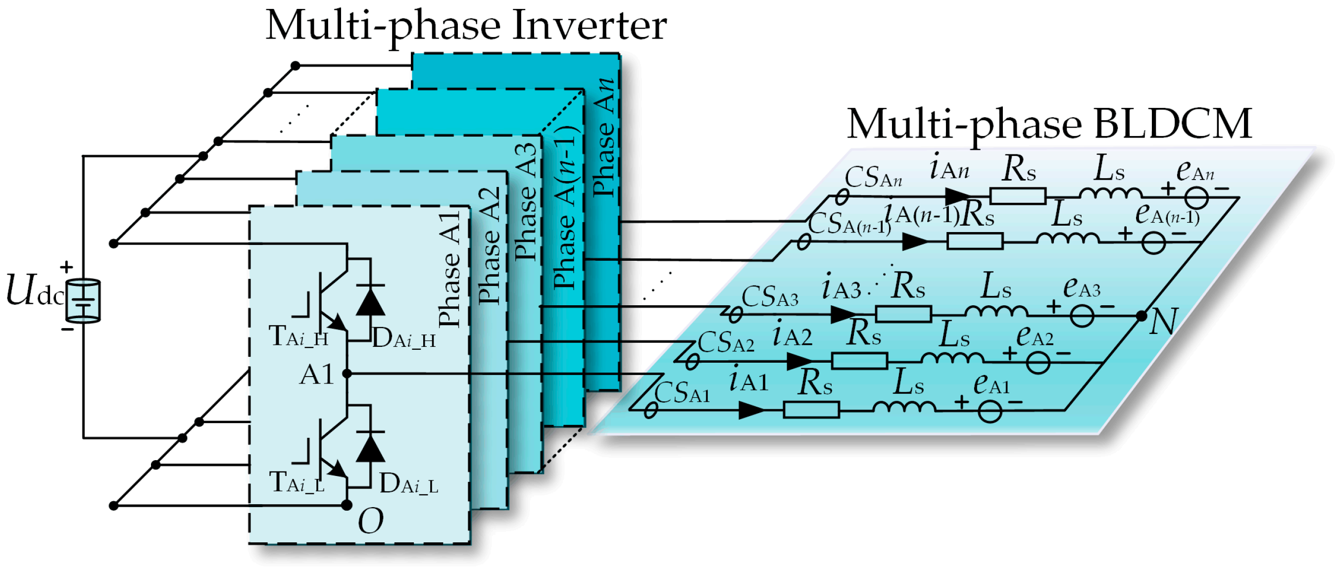
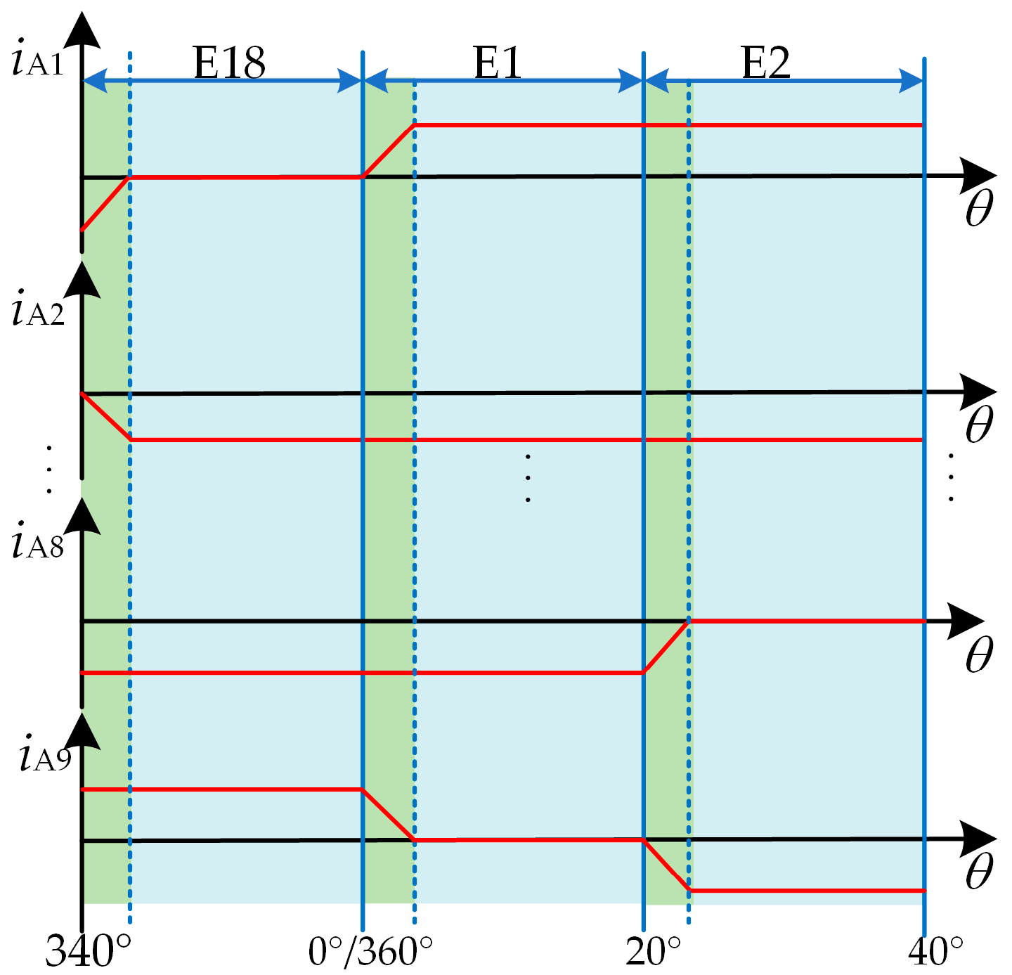
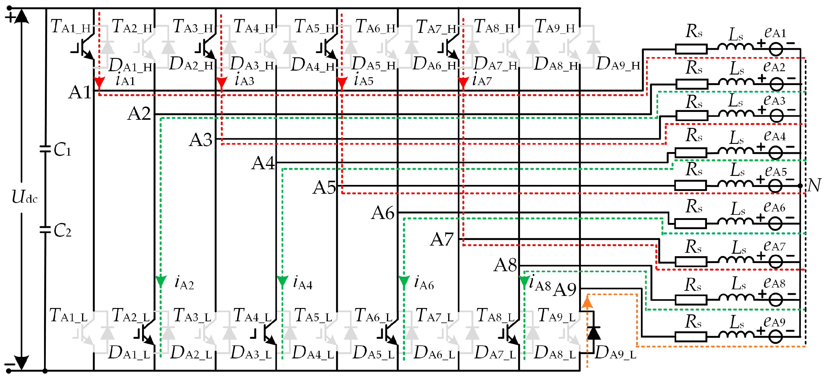
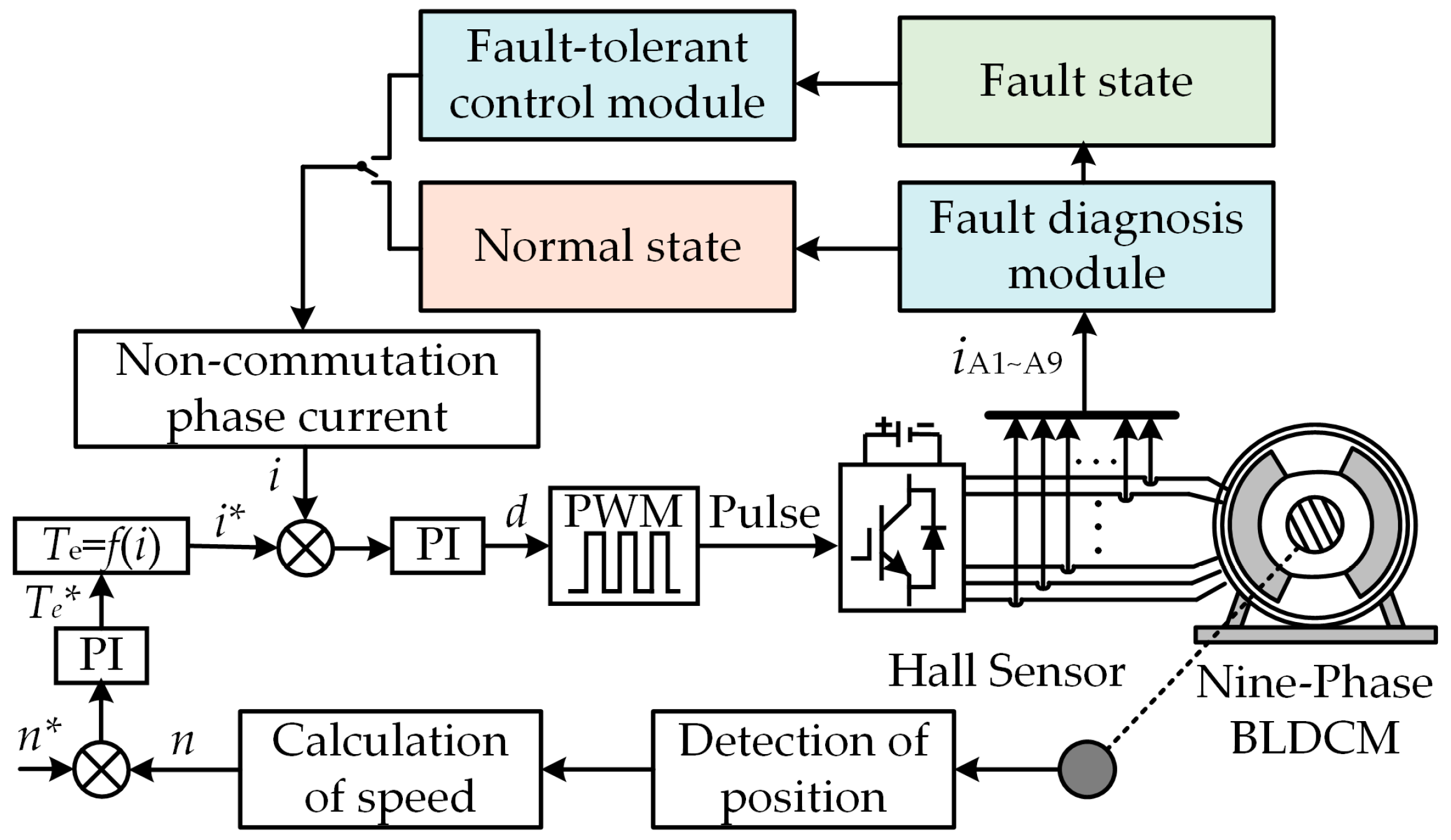
2.1. Operating Principle of Multiphase BLDCM Drive System

The equivalent circuit diagram of the symmetrical multiphase BLDCM drive system is displayed in Figure 1, where U_dc is the DC link voltage. The direction of the current flowing into the winding is defined as positive, and i_x (x = A1, A2, A3, …, An) is the x-phase current; CSx is a current sensor wrapped around the armature winding, directly measuring the nine-phase stator current; T_Ai__H and T_Ai__L (I = 1, 2, 3, …, n) represent the upper arm switch and lower arm switch of the voltage source inverter (VSI), respectively; D_Ai__H and D_Ai__L represent the upper arm and lower arm anti-parallel diodes of VSI, respectively. A1~An are phase windings, e_x is the reverse electromotive force of the motor, R_s is the resistance, L_s denote the self-inductance of armature winding, and N indicates the neutral point.

As shown in Figure 1, the voltage equation of the multiphase BLDCM is [6]:

$$\left\{\begin{array}{c}{u}_{\mathrm{A}1N}=R_s{i}_{\mathrm{A}1}+L_s{\displaystyle \frac{d{i}_{\mathrm{A}1}}{dt}}+e_{\mathrm{A}1}\\ u_{\mathrm{A}2N}=R_s{i}_{\mathrm{A}2}+L_s{\displaystyle \frac{d{i}_{\mathrm{A}2}}{dt}}+e_{\mathrm{A}2}\\ u_{\mathrm{A}3N}=R_s{i}_{\mathrm{A}3}+L_s{\displaystyle \frac{d{i}_{\mathrm{A}3}}{dt}}+e_{\mathrm{A}3}\\ ⋮\\ u_{\mathrm{A}(n-1)N}=R_s{i}_{\mathrm{A}(n-1)}+L_s{\displaystyle \frac{d{i}_{\mathrm{A}(n-1)}}{dt}}+e_{\mathrm{A}(n-1)}\\ u_{\mathrm{A}nN}=R_s{i}_{\mathrm{A}n}+L_s{\displaystyle \frac{d{i}_{\mathrm{A}n}}{dt}}+e_{\mathrm{A}n}\end{array}\right.$$

(1)

where i_A1~i_An are the motor phase currents; u_A1N~u_AnN are the motor phase voltages; n is the number of phases of the motor; and n > 3.

The armature windings are connected in a star configuration. Based on Kirchhoff’s current law, the phase currents satisfy the following relationship:

$$i_{\mathrm{A}1}+i_{\mathrm{A}2}+i_{\mathrm{A}3}+\cdots +i_{\mathrm{A}n}=0$$

(2)

The converted electromagnetic power acts on the load in the form of torque. Under ideal conditions, the electromagnetic torque can be expressed by the following equation:

$$P_e=T_e\omega$$

(3)

$$T_e={\displaystyle \frac{e_{\mathrm{A}1}{i}_{\mathrm{A}1}+e_{\mathrm{A}2}{i}_{\mathrm{A}2}+e_{\mathrm{A}3}{i}_{\mathrm{A}3}+\cdots +e_{\mathrm{A}n}{i}_{\mathrm{A}n}}{\omega }}$$

(4)

where ω represents the mechanical angular velocity.

However, as the number of phases in the symmetrical multiphase BLDCM increases, a larger back-EMF plateau width is required. For the sake of readability, this paper takes the nine-phase BLDCM as the analysis object. In order to achieve the best balance between torque output and system efficiency, the flat-top width is usually designed to be 160°, corresponding to an eight-phase conduction mode [6], as shown in Figure 2. In the nine-phase BLDCM, the back EMF of each phase presents a flat top width of 160°, ensuring the continuity of torque output when eight phases are turned on, where the flat top area corresponds to the winding conduction stage and the ramp area corresponds to the commutation transition. The current amplitude of the conducting phase is constant, and the floating phase current returns to zero after the commutation is completed. The current waveform is synchronized with the back EMF flat top area to optimize the electromagnetic torque. In addition, the jump edge (rising edge/falling edge) of the Hall signal accurately marks the commutation point, and the commutation is performed every 20° electrical angle. Therefore, the complete electrical cycle can be separated into 18 sectors according to the energized phase sequence. In each sector, four upper switches and four lower switches are simultaneously activated.

At the same time, the principle of dividing the Hall state into six sectors using binary combinations of Hall signals is similar to that in three-phase BLDCM [28]. The binary combination of the nine-phase BLDCM Hall signals is used to represent the Hall state, and it is divided into 18 working sectors within the 360° electrical angle, which are specifically defined as follows:

$$\begin{array}{l}{S}_{hall}=256\cdot H_1+128\cdot H_2+64\cdot H_3+32\cdot H_4\\ +16\cdot H_5+8\cdot H_6+4\cdot H_7+2\cdot H_8+1\cdot H_9\end{array}$$

(5)

where S_hall represents the current flow state of the motor. If it is in a healthy state, assuming clockwise direction, S_hall will repeat in the sequence shown in Figure 2 during the 360° electrical cycle. Among them, the Hall states 341 to 85 correspond to 18 sectors of the motor when it rotates clockwise. The conduction phase and the suspended phase corresponding to different Hall states are shown in

Table 1. The conduction phase and the suspended phase corresponding to different Hall states.

Hall State	Sector	Conduction Phase	Suspended Phase
341	E1	p = {A1,A3,A5,A7}; n = {A2,A4,A6,A8}	A9
340	E2	p = {A1,A3,A5,A7}; n = {A2,A4,A6,A9}	A8
342	E3	p = {A1,A3,A5,A8}; n = {A2,A4,A6,A9}	A7
338	E4	p = {A1,A3,A5,A8}; n = {A2,A4,A7,A9}	A6
346	E5	p = {A1,A3,A6,A8}; n = {A2,A4,A7,A9}	A5
330	E6	p = {A1,A3,A6,A8}; n = {A2,A5,A7,A9}	A4
362	E7	p = {A1,A4,A6,A8}; n = {A2,A5,A7,A9}	A3
298	E8	p = {A1,A4,A6,A8}; n = {A3,A5,A7,A9}	A2
426	E9	p = {A2,A4,A6,A8}; n = {A3,A5,A7,A9}	A1
170	E10	p = {A2,A4,A6,A8}; n = {A1,A3,A5,A7}	A9
171	E11	p = {A2,A4,A6,A9}; n = {A1,A3,A5,A7}	A8
169	E12	p = {A2,A4,A6,A9}; n = {A1,A3,A5,A8}	A7
173	E13	p = {A2,A4,A7,A9}; n = {A1,A3,A5,A7}	A6
165	E14	p = {A2,A4,A7,A9}; n = {A1,A3,A6,A8}	A5
181	E15	p = {A2,A5,A7,A9}; n = {A1,A3,A6,A8}	A4
149	E16	p = {A2,A5,A7,A9}; n = {A1,A4,A6,A8}	A3
213	E17	p = {A3,A5,A7,A9}; n = {A1,A4,A6,A8}	A2
85	E18	p = {A3,A5,A7,A9}; n = {A2,A4,A6,A8}	A1

, where p is the positive conduction phase and n is the negative conduction phase. It can be seen from Table 1 that during this entire electrical cycle, each phase armature winding is forward-conducted for 160° and reverse-conducted for 160°. Each commutation is performed between two phases, and the states of the other seven phase armature windings remain unchanged.

Taking the E18 sector switching to the E1 sector as an example for analysis, the two sectors can be obtained through (Table 1) the conducting phase and the suspended phase. Figure 3 shows the commutation area and non-commutation area of the nine-phase BLDCM at this stage.

In order to more clearly and intuitively show the difference between commutation and non-commutation, the E1 sector is divided into two parts: (1) The first part is the commutation area (green area), which is the E18 sector transition E1 sector stage. The A1 phase current gradually rises, and the A9 phase current continues to zero through the diode. The current path in this area is shown in Figure 4. At the beginning of commutation, the upper bridge arm T_{A1_H} of the A1 phase is turned on, and the current flows from the DC bus through the A1 phase to the neutral point; the A9 phase continues to flow through the lower bridge arm diode D_{A9_L}, and the current gradually decays to zero. Since the motor winding is inductive, the current on the winding cannot change suddenly during commutation, so that there is current in the nine-phase winding in the commutation interval. (2) The second part is the non-commutation area (blue area). In this stage, the positive conduction phase is turned on, and the negative conduction phase is turned on to form a closed loop. No current flows through the suspended phase A9. The current path in this area is shown in Figure 5. The above analysis shows that there are obvious differences in the current characteristics after sector switching. Therefore, a diagnostic method for current sensor zero-offset fault can be proposed based on the current change characteristics during sector switching.

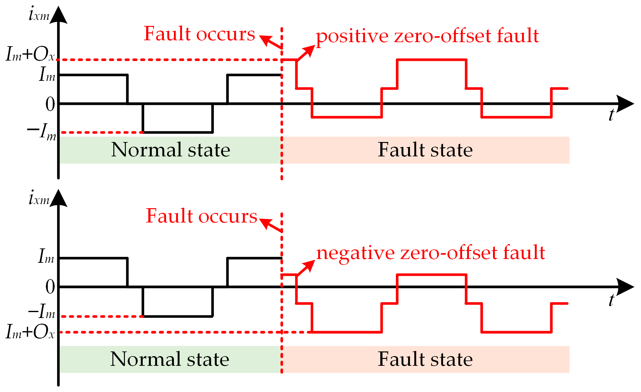
2.2. Analysis of Current Sensors Under Normal and Zero-Offset Fault Conditions

According to characteristics of the output signal of the current sensor zero-offset fault, the fault type can be divided into positive zero-offset fault and negative zero-offset fault. The schematic diagram of the two types of current states is shown in Figure 6, where I_m is the current amplitude. Under normal circumstances, the relationship between the phase current measured by the current sensor and the actual phase current satisfies:

$$i_{xm}=i_{xr}+O_{xf}$$

(6)

where i_xm is the phase current measured by the current sensor, i_xr is the actual phase current, and x represents each phase winding, that is, x∈{A1, A2, …, An}; O_xf is the zero-offset coefficient of the current sensor. When O_xf = 0, it indicates healthy state. When O_xf > 0, it indicates a positive zero-offset fault; when O_xf < 0, it indicates a negative zero-offset fault. As shown in Figure 6, whenever a zero-offset fault occurs, the current amplitude will change significantly compared to the normal state.

3. The Proposed Method

The proposed method is primarily composed of three parts: current sensor fault detection, zero-offset fault detection and location, and fault-tolerant control. Fault detection firstly detects whether a current sensor fault occurs in the corresponding stage. Subsequently, in the zero-offset fault detection and location stage, the detected fault type is identified and located. Fault-tolerant control is initiated when the diagnostic process is completed. These three parts are described in Section 3.1, Section 3.2 and Section 3.3, respectively.

3.1. Current Sensor Fault Detection

Firstly, the nine-phase currents are normalized to ensure that the current signal-based diagnostics are insensitive to load transients and are not affected by load level [16]. The maximum value of the nine-phase current amplitude is given by Equation (7); therefore, the normalized nine-phase current can be expressed as follows [18]:

$$i_{\max }=\max (\left|i_{\mathrm{A}1m}\right|,\left|i_{\mathrm{A}2m}\right|,\left|i_{\mathrm{A}3m}\right|,\cdots ,\left|i_{\mathrm{A}9m}\right|)$$

(7)

$$i_{xn}=i_{xm}/i_{\max }$$

(8)

Define the variable W in Equation (9) as the flag for current sensor fault detection:

$$W={\displaystyle \frac{1}{T_{\delta }}}{\displaystyle {\int }_{t_0}^{t_0+T_{\delta }}\left|i_{\mathrm{A}1n}+i_{\mathrm{A}2n}+i_{\mathrm{A}3n}+\cdots +i_{\mathrm{A}9n}\right|}dt$$

(9)

where T_δ is the sliding average period:

$$T_{\delta }=\delta T_f$$

(10)

Among them, T_f represents the fundamental period, which can be calculated by the real-time speed, and the parameter δ ∈ (0,1) defines the fundamental period part of the sliding average. In addition, due to the relatively high sampling frequency, even when the motor is running at maximum speed, enough sampling points can be collected within one fundamental wave cycle. Based on this, the influence of motor speed changes can be effectively eliminated through sliding average calculation.

In a Y-connected nine-phase BLDCM, the normal value of W should be equal to 0; otherwise, a ground fault or current sensor failure will occur. When a ground fault occurs, the differential protection device will force the drive system to shut down [18]. Therefore, W ≠ 0 can be used as a feature for fault detection. In order to avoid the influence of interference and measurement errors in the actual system, the threshold i_th1 is introduced, and the fault detection equation can be defined as follows:

$$F_d=\left\{\begin{array}{l}0,\left|W\right|\le i_{th1}\\ 1,\left|W\right|>i_{th1}\end{array}\right.$$

(11)

where F_d is the sign of fault occurrence; if F_d = 1, it indicates that there is a current sensor fault.

3.2. Zero-Offset Fault Detection and Localization

When a fault is detected, the subsequent normalized current change and the current change characteristics during the BLDCM sector switching process can be used to locate the zero-offset fault current sensor. The entire zero-offset fault detection and localization implementation process is divided into two parts: faulty sector judgment and fault location grounded in current change characteristics during sector switching.

(1) Determination of faulty sectors: To enable the online positioning of zero-offset fault, current amplitude detection variable R_x, rotor position angle θ, and Hall state S_hall are first introduced to judge the fault sector. Figure 7 shows the influence of zero-offset fault of the A1 phase current sensor on the absolute value of R_x under the normal operation of the A2~A9 phase current sensors, wherein the expression of R_x is as follows [15]:

$$R_x=\langle i_{xn}\rangle ={\displaystyle \frac{1}{T_{\delta }}}{\displaystyle {\int }_{t_0}^{t_0+T_{\delta }}{i}_{xn}dt}$$

(12)

In order to more clearly and intuitively judge the sector where each phase current sensor fault occurs, the sector judgment index S_x is defined, and its expression is as follows:

$$S_x=\left\{\begin{array}{l}1,\left|R_x\right|>\eta \cdot i_{\max \_avg}\\ 0,\left|R_x\right|\le \eta \cdot i_{\max \_avg}\end{array}\right.$$

(13)

where i_{max_avg} is the average value of the maximum absolute value of the nine-phase current within the unit fundamental wave period, as follows:

$$i_{max\_avg}={\displaystyle \frac{1}{T_{\delta }}}{\displaystyle {\int }_{t_0}^{t_0+T_{\delta }}\max (\left|i_{\mathrm{A}1m}\right|,\left|i_{\mathrm{A}2m}\right|,\cdots ,\left|i_{\mathrm{A}9m}\right|)dt}$$

(14)

where η is a constant preset value greater than zero; the range of η will be set to 0.01 to 0.02 as demonstrated by simulation and experiment.

Since the rotor position angle and Hall state corresponding to each sector in a multiphase BLDCM are fixedly allocated. Therefore, the sector in which the fault occurs can be determined by obtaining rotor position θ_f and the Hall state S_hall corresponding to when S_x = 1. Specifically, as shown in Figure 8, when the sector judgment index S_A1 = 1, the corresponding rotor position angle θ_f is between 80° and 100°, and the corresponding Hall state is 346, it can be determined that the fault occurs in the E5 sector.

To further obtain the offset value of the zero-offset fault, it can be expressed by defining the offset index K, as shown in Equation (15):

$$K={\displaystyle \frac{1}{T_{\delta }}}{\displaystyle {\int }_{t_0}^{t_0+T_{\delta }}(i_{\mathrm{A}1m}+i_{\mathrm{A}2m}+\cdots +i_{\mathrm{A}9m})dt=\delta }$$

(15)

where δ is the offset value of the faulty sensor. If the value of K stabilizes at a constant value that is not zero, it is determined that sensor occurs zero-offset fault. In addition, if fault occurs in a single-phase current sensor, the value of K is the phase offset value, that is, O_xf. If fault occurs simultaneously in multiphase current sensors, the value of K is the sum of the multiphase offset values.

In particular, the phase change control of the multiphase BLDCM is realized by the position signal collected by the Hall sensor. However, since the position signal is inherently discrete, rotor position information is provided only at the jump edge. Therefore, to obtain a continuous rotor position θ_t, the signal can be interpolated. Usually, the calculation is performed based on the jump edge and time information of the position signal. The expression is as follows:

$${\theta }_t={\theta }_{t-1}+\Delta \theta$$

(16)

where θ_t is the rotor position at moment t, and θ_t−1 is the corresponding rotor position angle along the last Hall signal jump adjacent to moment t; Δθ is the rotor angle position increment between two Hall signal jump edges, and its expression is as follows:

$$\Delta \theta ={\displaystyle \frac{2\pi }{N}}·{\displaystyle \frac{t_n-t_{n-1}}{T}}$$

(17)

where t_n denotes the current time of the system, and t_n−1 represents the time when the adjacent Hall signal transition edges occur; N is the total number of Hall signal state changes in one mechanical cycle, which depends on the configuration of the Hall signal and the number of pole pairs. In the nine-phase BLDCM, N = 18; T is the Hall jump cycle time.

(2) Zero-offset fault detection and localization based on current variation characteristics during sector switching: As analyzed in Section 2.1, each phase experiences a suspended state within one fundamental period.

Table 2. The rotor position angle corresponding to the suspended state of each phase winding within a unit fundamental wave period.

Fault Phase	Rotor Position Angle θc in Suspended State
A1	160° < θc < 180°; 340° < θc < 360°
A2	140° < θc < 160°; 320° < θc < 340°
A3	120° < θc < 140°; 300° < θc < 320°
A4	100° < θc < 120°; 280° < θc < 300°
A5	80° < θc < 100°; 260° < θc < 280°
A6	60° < θc < 80°; 240° < θc < 260°
A7	40° < θc < 60°; 220° < θc < 240°
A8	20° < θc < 40°; 200° < θc < 220°
A9	0° < θc < 20°; 180° < θc < 200°

illustrates the correspondence between the suspended state of each phase winding and the rotor position angle within one fundamental period. Taking phase A1 as an example, during sectors E9 and E18, phase A1 transitions into the suspended state following commutation. Normally, i_A1m will flow to zero after the commutation is completed, but if a zero-offset fault occurs in CS_A1, i_A1m will produce an offset O_A1f as shown in Figure 8 compared with the normal situation.

Taking CS_A1 as an example, when a zero-offset fault occurs, if it is detected that the faulty sector is between sectors E1 and E9, that is, after the commutation of sector E9 is completed, it is determined whether i_A1m is equal to zero for diagnosis. If it is detected that the faulty sector is between sectors E10 and E18, that is, after the commutation of sector E18 is completed, it is determined whether i_A1m is equal to zero to perform diagnosis.

Specifically, if the fault is detected to occur in sector E5, the phase change judgment can be performed in sector E9, as depicted in Figure 8. When operating normally, the current waveform of the E9 sector is shown in Figure 9a, and as analyzed above, the E9 sector is divided into a commutative region shown in the green area and a non-commutative region shown in the blue area according to whether it conducts or not. When fault occurs in CS_A1, the corresponding phase current does not decay to zero during sector E9; instead, it remains constant at a fixed offset value, denoted as O_A1f, as depicted in Figure 9b. Therefore, the end of commutation flag H_A1 and the zero-offset flag I_OA1 can be defined for the diagnosis of zero-offset faults. The expressions are as follows:

$$H_{\mathrm{A}1}=\left\{\begin{array}{l}0,\left|i_{\mathrm{A}1m}(n)-i_{\mathrm{A}1m}(n-1)\right|\le i_{th1}\\ 1,\left|i_{\mathrm{A}1m}(n)-i_{\mathrm{A}1m}(n-1)\right|>i_{th1}\end{array}\right.$$

(18)

$$I_{O\mathrm{A}1}=\left\{\begin{array}{l}1,\left|i_{\mathrm{A}1m}\right|>i_{th1}\\ 0,\left|i_{\mathrm{A}1m}\right|\le i_{th1}\end{array}\right.$$

(19)

where n and (n − 1) represent the current and previous sampling points, respectively; i_th1 is the threshold used to determine whether the current commutation has completed and to detect if the measured current exhibits an offset from zero after commutation completion. Normally, the value of |i_A1m| will not exceed 0.01A. Therefore, to ensure a certain safety margin, i_th1 is set to 0.05A to guarantee the reliability of the proposed method.

Based on the above analysis, the zero-offset fault diagnosis equation of CS_A1 is given as follows:

$$F_{O\mathrm{A}1}=F_d\wedge S_x\wedge H_{\mathrm{A}1}\wedge I_{O\mathrm{A}1}$$

(20)

where F_OA1 is the identification and localization flag of the CS_A1 zero-offset fault. If F_OA1 = 1, it signifies that CS_A1 occurs fault; if F_OA1 = 0, it signifies that CS_A1 is in a healthy state. Other phases can be analyzed in the same way. From Equation (21), the general equation for zero-offset fault diagnosis of each phase current sensor can be obtained:

$$F_{Ox}=F_d\wedge S_x\wedge H_x\wedge I_{Ox}$$

(21)

where F_Ox is the identification and localization flag of the CS_x zero-offset fault. Figure 10 presents the flowchart of the proposed method.

3.3. Fault-Tolerant Control

When the current sensor faults, if an effective fault-tolerant control strategy is not adopted in time, the strongly coupled motor system will be affected and the feedback signal will be distorted, thereby interfering with the motor operation state and even causing the motor system to crash. To address this issue, this section proposes a fault-tolerant control method based on current signal compensation for the zero-bias fault problem in the nine-phase current sensor.

For single-signal zero-bias faults, the zero-bias value can be estimated by the K value. However, for multi-signal faults, the zero-bias value cannot be estimated directly, so the repeated iteration method is used to gradually compensate for the fault. The compensation value is updated once per electrical cycle. First, diagnosis is performed according to Equation (21). If a fault is detected, R_x is calculated; then, the estimated compensation value of the faulty sensor is readjusted according to the following equation:

$$i_{\mathrm{A}x\_ft}=i_{\mathrm{A}xm}-O_{\mathrm{A}x\_est}^{k+1}$$

(22)

$$O_{\mathrm{A}x\_est}^{k+1}=O_{\mathrm{A}x\_est}^k+\mathrm{sign}(R_x)\times C_z$$

(23)

where i_{A1_ft} is the current after fault compensation; $O_{Ax\_est}^{k+1}$ indicates k + 1 compensation value; $O_{Ax\_est}^k$ indicates k compensation value; k is the number of iterations; C_z is a constant (C_z = 0.05A) used to determine the update rate of the compensation value $O_{Ax\_est}^{k+1}$; sign(R_x) indicates the direction of the offset (positive or negative). If the convergence condition |R_x| < i_th1 is met, the iteration is stopped. The fault-tolerant control of the zero-offset fault phase is achieved by compensating the offset value of the fault phase.

In order to conduct a sensitivity analysis of C_z, we set the range of C_z to 0.02~0.1 through experiments and simulations for verification and analyzed it from two dimensions, fault tolerance performance convergence time and steady-state error, and obtained a three-dimensional graph. As depicted in Figure 11, when C_z is too small, its convergence time becomes longer and longer, but the steady-state error will become smaller. However, if C_z is too large, the steady-state error will be too large and may even cause oscillation. This article sets it to 0.05 A, taking into account both response speed and stability.

The current sensor fault diagnosis and fault-tolerant control methods proposed are developed grounded in the operating principles of the nine-phase BLDCM. The method utilizes characteristics of normalized current averages and characteristics of current changes during sector switching to achieve fault diagnosis. Therefore, it is not only applicable to BLDCM but also to multiphase motors with other square wave control methods.

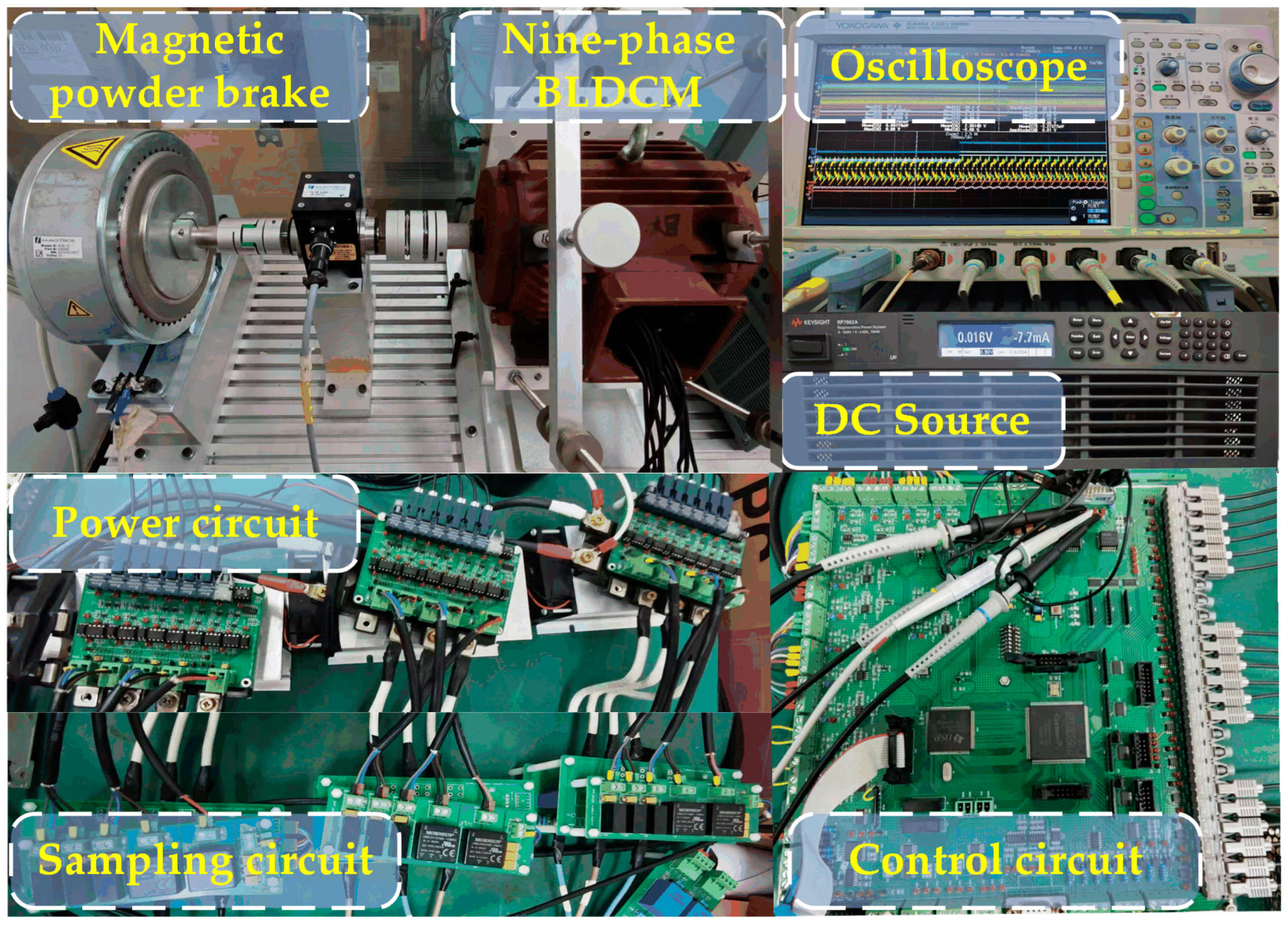
4. Experimental and Simulation Results Analysis

To validate the theoretical analysis, an experimental platform for the nine-phase BLDCM drive system was constructed, as illustrated in Figure 12. The control circuit uses DSP (TMS320F28335) and FPGA (EP1C6Q240C8) as the central control unit. The motor is loaded using a hysteresis brake, and the actual motor torque is measured using a torque sensor. The study subject is a 2 kW nine-phase BLDCM with symmetrical windings, and its parameters are presented in

Table 3. The parameters of a new symmetrical nine-phase brushless DC motor

Parameter	Symbol	Value
Rated voltage	UN	42.5 V
Rated power	PN	2 kW
Rated current	IN	23 A
Rated load	TN	8 N⋅m
Rated speed	nN	2500 r/min
Phase resistance	Rs	3.2 Ω
Phase inductance	Ls	0.064 mH
Phase back-EMF coefficient	Ke	0.06 V/(rad/s)
Pairs of poles	Pn	2

. To simulate the actual phenomena occurring when current sensor faults arise under various operating conditions, the output values of current sensors were artificially modified through software. All experiments were conducted under conditions of a DC bus voltage U_dc of 42 V, with both the sampling frequency and the switching frequency of the voltage source inverter set at 10 kHz.

The overall control block diagram of the proposed method is presented in Figure 13. The sampled current and rotor position angle are used for fault diagnosis. If the fault is detected and located, the system switches to the fault-tolerant control and uses fault-tolerant phase current as the system feedback current. Otherwise, the sampled current is used to implement closed-loop control.

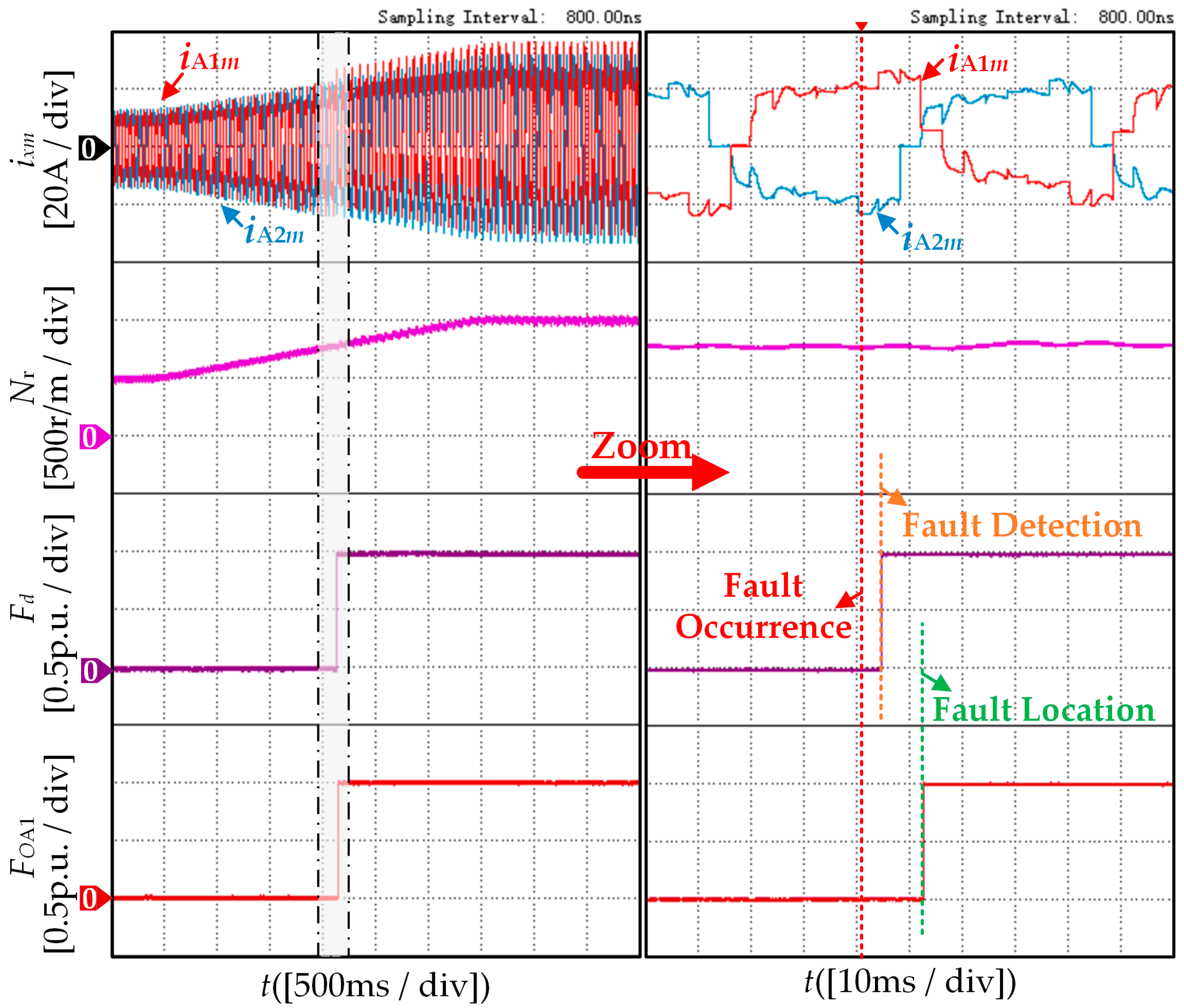
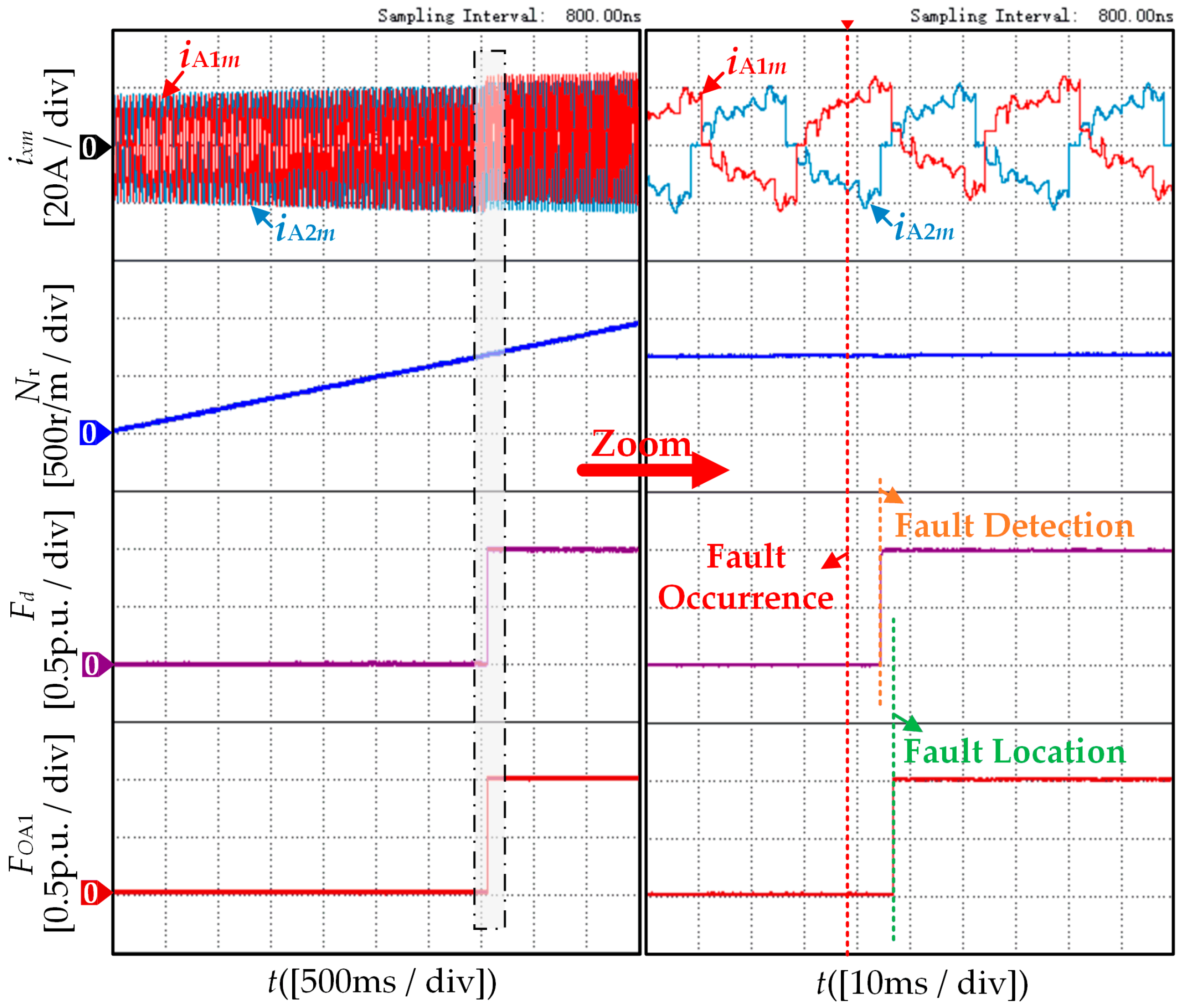
4.1. Validation of Robustness Results

To verify the robustness of the method, Experiments under different operating conditions were designed, and the results are depicted in Figure 14 and Figure 15, verifying the effectiveness of the method under load and speed variations. As depicted in Figure 14, under transient operating conditions, when the motor runs at a constant reference speed of 500 rpm and the load torque increases from 3 Nm to 8 Nm, the sampling current gradually increases. During this process, when a zero-offset fault occurs in CS_A1, the detection index F_d and the localization index F_Ox sequentially set to 1, indicating that the proposed method can achieve real-time detection and accurate localization of faults.

If the load torque is set to 4 N·m, the speed increases from 500 rpm to 1000 rpm; during this change process, CS_A1 also has a zero-offset fault, and the detection index F_d and the localization index F_Ox are set to 1 in turn, as shown in Figure 15. In summary, the experimental results verify that the proposed method can effectively avoid misdiagnosis under sudden change conditions and has good robustness.

4.2. Validation of Effectiveness Results

To verify whether this method is effective, this study carried out current sensor zero-offset fault diagnosis and fault tolerance experiments under steady-state operating conditions. The experimental setting is that the steady-state reference speed is 500 rpm, and the load torque is 4 Nm. Meanwhile specific offset is artificially applied to the sensor measurement value through software. The offset values selected in this experiment are 5 and −5, respectively.

Firstly, taking the zero-offset fault of CS_A1 as an example, Figure 16 illustrates diagnostic results for a zero-offset fault occurring in CS_A1 with an offset value of 5. As shown in Figure 16, when CS_A1 faults, the i_A1m exhibits a constant offset value greater than zero. Consequently, it can be concluded that a positive zero-offset fault has occurred. Among them, the detection index F_d changes from 0 to 1, the localization index F_OA1 changes from 0 to 1, and the detection variable K changes from 0 to 5, that is, the offset value of phase A1. It can be observed from the above results that the method can effectively diagnose the zero-offset fault of CS_A1 via the characteristic of whether i_A1m is zero at the end of the sector phase change as judged by the fault detection.

Figure 17 gives the diagnostic results of a zero-offset fault with an offset value of −5 occurring in CS_A1. As shown in Figure 17, the offset value K changes from 0 to −5, the detection indicator F_d changes from 0 to 1, and the localization indicator F_OA1 changes from 0 to 1, accurately locating the phase where the fault is located.

For the verification of the diagnostic effect of zero-offset faults occurring in multiple current sensors, this paper designs a positive zero-offset fault with an offset value of 5 occurring in CS_A1 and CS_A2 at the same time, and the diagnostic results are shown in Figure 18. It can be seen that when CS_A1 and CS_A2 faults occur, measured currents i_A1m as well as i_A2m in phases A1 and A2 have constant offset values. At this time, the detection index F_d changes from 0 to 1, and the detection variable K changes from 0 to 10, which is the sum of the offset values of all current sensors. The localization indicators F_OA1 and F_OA2 change from 0 to 1. In summary, the above analysis demonstrates that the proposed method effectively diagnoses both single-signal and multi-signal zero-offset faults.

In order to verify the influence of the minimum offset value, we conducted a zero-offset amplitude experiment in the range of 0-1A and found that the minimum zero-offset amplitude is about 1A. The diagnostic results of CS_A1 and CS_A2 for the minimum zero-offset amplitude are given below. As can be seen from Figure 19, when a fault occurs, the measured current of both is slightly offset and the torque fluctuation has little effect. However, the fault location indicators of both are triggered, which shows that the proposed method can have a certain diagnostic effect on the minimum offset amplitude.

In addition, to verify the performance of the proposed fault-tolerant method, the zero-offset fault of the A1 phase current sensor is taken as an example. In particular, to more clearly and intuitively reflect effect of fault-tolerant control after a fault, the experiment is set to start the fault-tolerant control strategy about 1~1.5 s after the fault diagnosis is completed. Figure 20 shows the effect of fault-tolerant control of CS_A1 under steady state operation. As can be seen, the current amplitude as well as the torque after the fault-tolerant control is consistent with the normal condition. Figure 21 demonstrates the fault-tolerant control effect of CS_A1 and CS_A2 after simultaneous zero-offset faults under steady state operation, the analysis is the same as the above and will not be elaborated here.

In order to demonstrate the fault-tolerant effect under other offset values, Figure 22 shows the fault-tolerant effect of CS_A1 with an offset value of 10. When the offset value is 10, the torque fluctuation is large, but the method can effectively reduce the torque fluctuation and maintain the stable operation of the system. In order to more comprehensively demonstrate the torque fluctuation performance after fault-tolerant control,

Table 4. Fault tolerance performance under different working conditions.

Fault Phase	Offset Value	Tef	Teft	Reduction
A1	5A	14.5%	11.8%	2.7%
A1	10A	27.2%	21%	6.2%
A1 and A2	5A	20.25%	18%	2.25%

summarizes the torque fluctuation comparisons under fault conditions and fault-tolerant control under different working conditions. Among them, Te_f represents the torque fluctuation rate under fault conditions, and Te_ft represents the torque fluctuation rate under fault-tolerant conditions, which is calculated by the percentage of torque ripple ΔT_e under each working condition to the operating torque. As can be seen from Table 4, through fault-tolerant control, the torque fluctuation of the system has been significantly improved, and the torque fluctuation rate under fault-tolerant conditions is generally controlled at about 5% of the fault condition, indicating that our fault-tolerant control method can effectively reduce torque fluctuations under different working conditions.

4.3. Simulation Results Analysis

To better understand the feasibility of the proposed method in a practical environment, this paper takes the influence of winding fault, multiphase fault, and Hall position signal deviation interference as examples to analyze. Figure 23 shows the distinguishing between zero-offset faults and winding open-circuit faults. The currents of zero-offset faults and open-circuit faults have obvious changes. The difference is that the current amplitude of zero-bias faults increases or decreases, while the current of open-circuit faults gradually approaches zero. As shown in Figure 23a, after the zero-bias fault, the detection index W jumps from zero, while after the open-circuit fault, W remains unchanged, as shown in Figure 23b. Therefore, it can be shown that the fault detection index can effectively distinguish between winding faults and current sensor faults. Figure 24 shows the diagnostic effect of multiple phase faults. The current amplitudes of multiple phases change at the same time, but the fault characteristics of each phase can still be identified.

In addition, to better verify the robustness of the method to the Hall signal deviation, a simulation test was carried out by introducing the Hall signal error model. Figure 25 shows the fault diagnosis results of the Hall deviation of phase A1. It can be seen from the figure that when the Hall deviation is 5°, the rotor position angle has a significant offset; under this condition, when CS_A1 has a zero-bias fault, the fault indicator can be effectively triggered. By means of simulation analysis, it can determined that the proposed method can provide better robustness and stability and can effectively avoid misjudgment caused by noise or other interference factors when relying only on a single-phase current indicator.

5. Conclusions

In this paper, an effective method for zero-offset fault diagnosis and tolerant control of current sensors is proposed for multiphase BLDCM drive systems. Firstly, based on the measured current variations under zero-offset fault conditions in current sensors, this method establishes an integrated fault diagnosis framework, which exhibits consistent fault detection and localization performance in zero-offset fault mode. Subsequently, a tolerant control method is designed by analyzing the current trend under the zero-offset fault scenario. The proposed method operates without the need for any additional hardware components or utilization of motor parameters, making it suitable for rapid integration into mature motor drives. Finally, this paper conducts experiments on a symmetrical nine-phase BLDCM drive system platform. The experimental results show that the average diagnosis time of the proposed method is 0.2 fundamental wave cycles. Compared with previous research methods [24,26], it has a faster diagnosis speed. The torque fluctuation after fault tolerance is reduced by less than 5%, thereby confirming the reliability and performance of the proposed approach. The main contributions of this paper are as follows:

(1)

The proposed method is based on the current variation characteristics, so it has strong robustness and simple implementation.

(2)

The method accurately estimates the fault coefficients under current sensor faults and compensates for faulty current sensors, realizing fault-tolerant operation of the system.

(3)

The proposed method has been experimentally proven to be effective in a nine-phase BLDCM system and possesses scalability for application in systems with analogous square-wave driving structures. However, in practical applications, it still needs to be combined with specific structural adaptability design.

References

1. Barrero, F.; Duran, M.J. Recent advances in the design, modeling, and control of multiphase machines—Part I. IEEE Trans. Ind. Electron. 2015, 63, 449–458. [Google Scholar] [CrossRef]
2. Duran, M.J.; Barrero, F. Recent advances in the design, modeling, and control of multiphase machines—Part II. IEEE Trans. Ind. Electron. 2015, 63, 459–468. [Google Scholar] [CrossRef]
3. Bodo, N.; Levi, E.; Subotic, I.; Espina, J.; Empringham, L.; Johnson, C.M. Efficiency evaluation of fully integrated on-board EV battery chargers with nine-phase machines. IEEE Trans. Energy Convers. 2016, 32, 257–266. [Google Scholar] [CrossRef]
4. Salem, A.; Narimani, M. A review on multiphase drives for automotive traction applications. IEEE Trans. Transp. Electrific. 2019, 5, 1329–1348. [Google Scholar] [CrossRef]
5. Frikha, M.A.; Croonen, J.; Deepak, K.; Benômar, Y.; El Baghdadi, M.; Hegazy, O.J.E. Multiphase motors and drive systems for electric vehicle powertrains: State of the art analysis and future trends. Energies 2023, 16, 768. [Google Scholar] [CrossRef]
6. Chen, W.; Zhu, L.; Li, X.; Shi, T.; Xia, C. Comparing the performance of parallel multi-phase brushless dc motors: A comprehensive analysis. IEEE Trans. Power Electron. 2023, 38, 11290–11303. [Google Scholar] [CrossRef]
7. Park, H.; Kim, T.; Suh, Y. Fault-tolerant control methods for reduced torque ripple of multiphase BLDC motor drive system under open-circuit faults. IEEE Trans. Ind. Electron. 2022, 58, 7275–7285. [Google Scholar] [CrossRef]
8. Choi, K.; Kim, Y.; Kim, S.-K.; Kim, K.-S. Current and position sensor fault diagnosis algorithm for PMSM drives based on robust state observer. IEEE Trans. Ind. Electron. 2020, 68, 5227–5236. [Google Scholar] [CrossRef]
9. Zhang, G.; Wang, G.; Wang, G.; Huo, J.; Zhu, L.; Xu, D. Fault diagnosis method of current sensor for permanent magnet synchronous motor drives. In Proceedings of the 2018 International Power Electronics Conference (IPEC-Niigata 2018—ECCE Asia), Niigata, Japan, 20–24 May 2018; pp. 1206–1211. [Google Scholar] [CrossRef]
10. Attaianese, C.; D’Arpino, M.; Di Monaco, M.; Di Noia, L.P. Current signature modeling of surface-mounted PMSM drives with current sensors faults. IEEE Trans. Energy Convers. 2023, 38, 2695–2705. [Google Scholar] [CrossRef]
11. Chung, D.-W.; Sul, S.-K. Analysis and compensation of current measurement error in vector-controlled AC motor drives. IEEE Trans. Ind. Appl. 1998, 34, 340–345. [Google Scholar] [CrossRef]
12. Lee, K.-W.; Kim, S.-I.J. Dynamic performance improvement of a current offset error compensator in current vector-controlled SPMSM drives. IEEE Trans. Ind. Electron. 2018, 66, 6727–6736. [Google Scholar] [CrossRef]
13. Foo, G.H.B.; Zhang, X.; Vilathgamuwa, D.M. A sensor fault detection and isolation method in interior permanent-magnet synchronous motor drives based on an extended Kalman filter. IEEE Trans. Ind. Electron. 2013, 60, 3485–3495. [Google Scholar] [CrossRef]
14. Yu, Y.; Zhao, Y.; Wang, B.; Huang, X.; Xu, D. Current sensor fault diagnosis and tolerant control for VSI-based induction motor drives. IEEE Trans. Power Electron. 2017, 33, 4238–4248. [Google Scholar] [CrossRef]
15. Huang, P.; Liu, J.; Wang, J. Fault Diagnosis for Current Sensors in Charging Modules Based on an Adaptive Sliding Mode Observer. Sensors 2025, 25, 1413. [Google Scholar] [CrossRef]
16. Attaianese, C.; D’Arpino, M.; Di Monaco, M.; Di Noia, L.P. Model-based detection and estimation of dc offset of phase current sensors for field oriented PMSM drives. IEEE Trans. Ind. Electron. 2023, 70, 6316–6325. [Google Scholar] [CrossRef]
17. Attaianese, C.; D’Arpino, M.; Di Monaco, M.; Di Noia, L.P. Isolation, Detection and Estimation of Current Sensors Faults in PMSM Drives Based on Current Signature Modeling. IEEE Trans. Energy Convers. 2024, 40, 653–664. [Google Scholar] [CrossRef]
18. El Khil, S.K.; Jlassi, I.; Cardoso, A.J.M.; Estima, J.O.; Mrabet-Bellaaj, N. Diagnosis of open-switch and current sensor faults in PMSM drives through stator current analysis. IEEE Trans. Ind. Appl. 2019, 55, 5925–5937. [Google Scholar] [CrossRef]
19. Lu, J.; Hu, Y.; Chen, G.; Wang, Z.; Liu, J. Mutual calibration of multiple current sensors with accuracy uncertainties in IPMSM drives for electric vehicles. IEEE Trans. Ind. Electron. 2020, 67, 69–79. [Google Scholar] [CrossRef]
20. Wu, C.; Guo, C.; Xie, Z.; Ni, F.; Liu, H. A signal-based fault detection and tolerance control method of current sensor for PMSM drive. IEEE Trans. Ind. Electron. 2018, 65, 9646–9657. [Google Scholar] [CrossRef]
21. Chakraborty, C.; Verma, V. Speed and current sensor fault detection and isolation technique for induction motor drive using axes transformation. IEEE Trans. Ind. Electron. 2014, 62, 1943–1954. [Google Scholar] [CrossRef]
22. Wang, G.; Hao, X.; Zhao, N.; Zhang, G.; Xu, D. Current sensor fault-tolerant control strategy for encoderless PMSM drives based on single sliding mode observer. IEEE Trans. Transport. Electrific. 2020, 6, 679–689. [Google Scholar] [CrossRef]
23. Zhang, G.; Zhou, H.; Wang, G.; Li, C.; Xu, D. Current sensor fault-tolerant control for encoderless IPMSM drives based on current space vector error reconstruction. IEEE J. Emerg. Sel. Topics Power Electron. 2019, 8, 3658–3668. [Google Scholar] [CrossRef]
24. Ma, G.; Zhang, H.; Sun, Z.; Yao, C.; Ren, G.; Xu, S. Current sensor fault localization and identification of PMSM drives using difference operator. IEEE J. Emerg. Sel. Topics Power Electron. 2023, 11, 1097–1110. [Google Scholar] [CrossRef]
25. Feng, X.; Wang, B.; Wang, Z.; Hua, W. Investigation and Diagnosis of Current Sensor Fault in Permanent Magnet Machine Drives. IEEE Trans. Ind. Electron. 2024, 72, 1261–1270. [Google Scholar] [CrossRef]
26. Zhang, Y.; Zhou, B.; Fang, W.; Chen, W. A fault diagnosis method for current sensor of doubly salient electromagnetic motor. IEEE Trans. Ind. Electron. 2023, 71, 4419–4428. [Google Scholar] [CrossRef]
27. Fang, W.; Zhou, B.; Zhang, Y.; Yu, X.; Jiang, S.; Wei, J. A Fault Diagnosis and Fault-Tolerant Control Method for Current Sensors in Doubly Salient Electromagnetic Motor Drive Systems. IEEE J. Emerg. Sel. Topics Power Electron. 2024, 12, 2234–2248. [Google Scholar] [CrossRef]
28. Dong, L.; Jatskevich, J.; Huang, Y.; Chapariha, M.; Liu, J. Fault diagnosis and signal reconstruction of hall sensors in brushless permanent magnet motor drives. IEEE Trans. Energy Convers. 2015, 31, 118–131. [Google Scholar] [CrossRef]
Figure 1. Equivalent circuit diagram of multiphase BLDCM drive system.
Energies 18 02243 g001
Figure 2. The nine-phase BLDCM uses the eight-phase conduction method to show the phase relationship between the back electromotive force, phase current, and Hall signal.
Energies 18 02243 g002
Figure 3. Schematic diagram of the commutation and non-commutation regions of a nine-phase BLDCM.
Energies 18 02243 g003
Figure 4. Schematic diagram of the current path in the commutation area of sector E1 (Red indicates positively conducting phase current paths, green indicates negatively conducting phase current paths, and orange indicates suspended phase current paths).
Energies 18 02243 g004
Figure 5. Schematic diagram of current path in non-commutation area of sector E1 (Red indicates positively conducting phase current paths, green indicates negatively conducting phase current paths).
Energies 18 02243 g005
Figure 6. Current sensor zero-offset fault state.
Energies 18 02243 g006
Figure 7. Influence of zero-offset fault on |Rx|.
Energies 18 02243 g007
Figure 8. Zero-offset fault sector determination.
Energies 18 02243 g008
Figure 9. Phase A1 current characteristics in sector E9; (a) Normal state; (b) Zero-offset Fault.
Energies 18 02243 g009
Figure 10. Flowchart of the proposed method.
Energies 18 02243 g010
Figure 11. Cz sensitivity analysis.
Energies 18 02243 g011
Figure 12. Nine-phase BLDCM drive system experiment platform.
Energies 18 02243 g012
Figure 13. Control block diagram of the proposed method.
Energies 18 02243 g013
Figure 14. Experimental results under the load variation.
Energies 18 02243 g014
Figure 15. Experimental results under the speed variation.
Energies 18 02243 g015
Figure 16. Positive zero-offset fault diagnosis results of the CSA1.
Energies 18 02243 g016
Figure 17. Negative zero-offset fault diagnosis results of the CSA1.
Energies 18 02243 g017
Figure 18. Positive zero-offset fault diagnosis results of the CSA1 and CSA2.
Energies 18 02243 g018
Figure 19. Minimum zero-offset fault diagnosis results of the CSA1 and CSA2.
Energies 18 02243 g019
Figure 20. Positive zero-offset fault tolerance control of the CSA1.
Energies 18 02243 g020
Figure 21. Positive zero-offset fault tolerance control of the CSA1 and CSA2.
Energies 18 02243 g021
Figure 22. The fault tolerance effect of a CSA1 offset value of 10.
Energies 18 02243 g022
Figure 23. Distinguishing between zero-offset fault and winding open-circuit fault; (a) Zero-offset fault; (b) Winding open-circuit fault.
Energies 18 02243 g023
Figure 24. Multiphase fault diagnosis results.
Energies 18 02243 g024
Figure 25. Hall sensor misalignment interference.
Energies 18 02243 g025