Article

Recovery Strategy of Distribution Network Based on Power Supply Capability Assessment of Local Area Configured with Energy Gateway

by
Xiaoxia Guo
1,
Weijia Guo
2,
Xiang Jiang
1,
Wei Wang
1 and
Junpeng Zhu
2,*
1
Rugao Power Supply Company, State Grid Jiangsu Electric Power Co., Ltd., Nantong 226503, China
2
School of Electrical and Power Engineering, Hohai University, Nanjing 210098, China
*
Author to whom correspondence should be addressed.
Energies 2025, 18(9), 2215; https://doi.org/10.3390/en18092215
Submission received: 21 March 2025 / Revised: 19 April 2025 / Accepted: 20 April 2025 / Published: 27 April 2025

Abstract

:
The growing integration of DG enhances distribution network resilience, but existing centralized fault recovery strategies face critical limitations: excessive computational burdens on DCs and the insufficient utilization of local control capabilities, particularly with large-scale DG deployments. Current studies often fail to balance computational efficiency and dynamic recovery coordination between centralized and decentralized resources. To address the issue, a hierarchical control architecture is proposed that involves collaboration between the DC and LA energy gateways. By dynamically quantifying LA PSC through net power feasibility analysis, the framework optimizes network reconfiguration (DC level) and decentralized DG scheduling (gateway level). Validated on a modified IEEE 45-bus system, the strategy restored 7 MWh (4:00 fault) and 5 MWh (10:00 fault) of load, outperforming static methods by 26.9× in the mid-day case. While effective in urban grids, rural DG-sparse areas require future integration of mobile storage. The work balances centralized coordination and decentralized execution, offering a scalable resilience solution for modern networks.

1. Introduction

The increasing frequency of extreme weather events, coupled with the rapid integration of DG, has underscored the critical need for resilient power distribution networks. Recent blackouts, such as the 2021 Texas winter storm [1], the 2022 Taiwan outage [2], and the 2023 Pakistan grid collapse [3], have exposed vulnerabilities in conventional grid recovery strategies. These events highlight a pressing challenge: traditional centralized fault recovery mechanisms struggle to balance computational efficiency with the dynamic coordination required in modern grids enriched with DG, including PV technologies, ESSs, and NBSUs. While DG offers significant potential for post-blackout recovery [4], its large-scale deployment introduces complexities in resource coordination, network reconfiguration, and real-time decision making, necessitating innovative solutions to enhance grid resilience.
Existing research has explored various approaches to address these challenges. Centralized optimization frameworks, such as those proposed in [5,6,7], rely on DCs to coordinate all DG technologies and switches. However, these methods suffer from exponential computational growth as DG penetration increases, leading to impractical solving times during emergencies. Decentralized strategies, such as microgrid-based islanding [6] and layered architectures [7], mitigate computational burdens but often sacrifice global optimality or require complex boundary adjustments. Recent advancements in flexibility modeling, including Thevenin equivalents [8] and projection-based feasible regions [9], aim to simplify multi-region coordination. However, high-dimensional constraints and redundant security conditions [10,11] limit their scalability. Furthermore, while studies like [12] emphasize operator interaction in regional energy systems, they overlook the autonomous capabilities of local controllers. A critical gap persists in harmonizing centralized oversight with decentralized execution, particularly in dynamically assessing local PSCs to enable efficient resource allocation.
The concept of TSC [13,14,15,16,17,18,19] has been widely adopted for contingency analysis, yet its application to DG-rich networks remains limited. For instance, Xu et al. [18] evaluated PSC under reliability constraints but did not integrate real-time DG variability. Similarly, Silva et al. [20] proposed TSO-DSO flexibility estimation but omitted hierarchical control mechanisms. Recent work by Chen et al. [16] optimized load ability curves but relied on static models incompatible with dynamic restoration phases. These limitations underscore a fundamental research question: How can distribution networks achieve computationally efficient, scalable recovery while fully leveraging localized DG capabilities during blackouts? This question branches into sub-problems: (1) how to decouple centralized and decentralized control tasks to reduce DC computational burdens; (2) how to dynamically quantify and utilize LA-specific PSC for optimal net power planning; and (3) how to ensure seamless coordination between network topology adjustments and DG scheduling?
Motivated by these challenges, this paper proposes a hierarchical recovery strategy grounded in PSC assessment. Our work diverges from prior studies by introducing a two-tier architecture, where DCs optimize high-level network topology and net power plans, while energy gateways at LAs autonomously schedule DG based on locally feasible regions. This approach builds on the umbrella constraint reduction framework [11] and integrates advancements in linearized mixed-integer programming [21]. Notably, we extend the concept of TSC to DG-dominated LAs, enabling dynamic PSC quantification through reactive power decoupling, a novel contribution that addresses the rigidity of traditional TSC models [22,23,24]. Additionally, we incorporate insights from recent studies on hybrid AC/DC microgrid resilience [25], which emphasize the role of localized control in mitigating communication failures.
The remainder of this paper is organized as follows: Section 2 details the hierarchical control architecture; Section 3 formalizes the PSC assessment methodology; Section 4 presents the recovery strategy; Section 5 validates the approach through simulations; Section 6 analyzes the achievements of this work; and Section 7 describes the main results achieved in quantitative and qualitative forms and adds the weaknesses of the proposed methodology, existing limitations, and possible future research. By bridging the gap between centralized optimization and decentralized execution, this work advances the state of the art in grid resilience, offering a scalable solution for DG-rich urban networks.

2. Hierarchical Control Architecture

2.1. The Subsection of the Distribution System Equipped with Energy Gateways

The distribution system illustrated in Figure 1 consists of multiple areas, each equipped with an energy gateway, where the DC serves as the central control point, managing switches and DG technologies by communicating with DTUs, FTUs, and the respective energy gateway for each LA. The energy gateway serves as a communication interface between the DC and the LA it serves. When the DC sends commands to alter switches, the network topology undergoes changes, facilitated by the collaboration between DTUs and FTUs. The energy gateway of each LA generates schedules for DG based on the commands received from the DC. This ensures the efficient operation and output of DG within each LA. The system configuration enables effective communication, control, and coordination, thereby guaranteeing a reliable power supply to the loads in the network. The hardware configuration of energy gateways is detailed in Table 1, and the communication protocol complies with the IEC 60870-5-104 standard [26].

2.2. The Information-Sharing Framework of a Distribution System Equipped with Energy Gateways

The information-sharing framework in Figure 2 is a key component of the distribution system, involving the DC, gateways, and clients. The DC collects dates from gateways to assess the LAs’ PSCs and design SRPs after blackouts, designing their net power plans.
Post-blackout, gateways collect historical data, real-time information, and power forecasts from clients. This dataset is used to calculate parameters for the DC, enabling informed decisions on SRP implementation. Gateways implement DC-provided SRPs and schedule DG within LAs.

3. Power Supply Capability Assessment of LAs

Assuming B PVs, C ESSs, and E NBSUs operate within the LA, the NBSUs managed by the same energy gateway start to generate energy simultaneously.

3.1. PSC Method of LAs

The PSC of LAs transmitted from gateways to the DC is represented by parameter set D, defined as follows:
D = { p i , 1 L , p i , 2 L , , p i , T L , q i , 1 L , q i , 2 L , , q i , T L , ζ i , 1 P V , ζ i , 2 P V , , ζ i , T P V , E i E S S , C h a r , E i E S S , D i s } ,
The method to calculate each element in set D is as follows:
ζ i , t P V = ( b = 1 B S i , b P V ζ i , t , b P V ) / ( b = 1 B S i , b P V )
E i E S S , C h a r = c = 1 C E i , c E S S , C h a r
E i E S S , D i s = c = 1 C E i , c E S S , D i s

3.2. Parameters Stored in DC

When developing SRPs, the DC should rely on locally stored parameters, calculated as follows:
S i P V = b = 1 B S i , b P V
S i E S S = c = 1 C S i , c E S S
S i N B S U = e = 1 E S i , e N B S U
S i , min E S S = min { S i , 1 E S S , S i , 2 E S S , , S i , C E S S }
p i N B S U , d o w n = min { p i , 1 N B S U , d o w n , p i , 2 N B S U , d o w n , , p i , E N B S U , d o w n }
p i N B S U , u p = min { p i , 1 N B S U , u p , p i , 2 N B S U , u p , , p i , E N B S U , u p }
T i N B S U = max { T i , 1 N B S U ,     T i , 2 N B S U ,   , T i , E N B S U }
p i N B S U , i n = ( e = 1 E T i , e N B S U p i , e N B S U , i n ) / T i N B S U

3.3. The Feasible Regions of p i , t / q i , t Defined by PSC of LAs

A DC uses feasible regions with smaller dimensions and fewer constraints, defined by LA PSCs, for centralized control. These regions are:
Ω D C , n e t = ( p i , t , q i , t ) s . t . E q u a t i o n ( 13 )
0 . 31 ( S i P V + S i E S S + S i N B S U ) q i , t + q i , t L 0 . 31 ( S i P V + S i E S S + S i N B S U )
p i , t + p i , t L = p i , t P V + p i , t E S S + p i , t N B S U
0 p i , t P V X i , t 1 ζ i , t P V S i P V
S i , min E S S p i , t E S S S i , min E S S
E i E S S , C h a r Δ t t = 1 d p i , t E S S E i E S S , D i s 1 d T
μ i , t N B S U M t i N B S U t 1 μ i , t N B S U M
φ i , t N B S U M t i N B S U + T i N B S U t 1 φ i , t N B S U M
μ i , t N B S U φ i , t N B S U X i , t
0 p i , t N B S U ( φ i , t N B S U μ i , t N B S U ) p i N B S U , i n φ i , t N B S U S i N B S U
φ i , t N B S U 1 M p i N B S U , d o w n p i , t + 1 N B S U p i , t N B S U 1 φ i , t N B S U M + p i N B S U , u p

3.4. The Actual Feasible Regions of DG in LAs

Ignoring ESS charge/discharge losses, the feasible range for DG’s actual PSC within LAs is defined as:
Ω L A = ( p i , t , q i , t ) s . t . E q u a t i o n ( 14 ) ,   E q u a t i o n ( 15 ) , E q u a t i o n ( 16 ) , E q u a t i o n ( 17 )
p i , t = b = 1 B p i , t , b P V + c = 1 C p i , t , c E S S + e = 1 E p i , t , e N B S U p i , t L
q i , t = b = 1 B q i , t , b P V + c = 1 C q i , t , c E S S + e = 1 E q i , t , e N B S U q i , t L
2 S i , b P V p i , t , b P V ± q i , t , b P V 2 S i , b P V
S i , b P V cos φ max q i , t , b P V S i , b P V cos φ max
0 p i , t , b P V X i , t 1 ζ i , t , b P V S i , b P V
2 S i , c E S S p i , t , c E S S ± q i , t , c E S S 2 S i , c E S S
S i , c E S S cos φ max q i , t , c E S S S i , c E S S cos φ max
S i , c E S S p i , t , c E S S S i , c E S S
E i , c E S S , C h a r Δ t t = 1 d p i , t , c E S S E i , c E S S , D i s 1 d T
2 S i , e N B S U p i , t , e N B S U ± q i , t , e N B S U 2 S i , e N B S U
S i , e N B S U q i , t , e N B S U S i , e N B S U
μ i , t , e N B S U M t i , e N B S U t 1 μ i , t , e N B S U M
φ i , t , e N B S U M t i , e N B S U + T i , e N B S U t 1 φ i , t , e N B S U M
μ i , t , e N B S U φ i , t , e N B S U X i , t
0 p i , t , , e N B S U ( φ i , t , e N B S U μ i , t , e N B S U ) p i , e N B S U , i n φ i , t , e N B S U S i , e N B S U
φ i , t , , e N B S U 1 M p i , e N B S U , d o w n p i , t + 1 , e N B S U p i , t , e N B S U 1 φ i , t , e N B S U M + p i , e N B S U , u p
where φ max is the upper limit of the power factor angle of PVs and ESSs, and the value of cos φ max is 0.31.
Proof. 
The Net Power Plans Formulated by a DC All Can Be Implemented by Las. □
The transformation from Equations (14)–(17) to Equation (15) is outlined here, emphasizing that Equation (15) is a sufficient condition for Equations (14)–(17), i.e., Ω D C , n e t Ω L A , n e t .
Detailed derivations of the feasible regions are provided in Appendix A.

4. The Recovery Strategy of a Distribution Network

The recovery strategy of a distribution network includes an upper-level DC model and lower-level LA energy gateway models. The upper-level model determines the dynamic network topology and the net power plants, whereas the lower-level model schedules DG.

4.1. The Upper-Level Model for a DC

4.1.1. Objective Function

The objective function F1, defined in Equation (18), calculates the post-blackout load saved and switch operating costs.
F 1 = t = 1 T i = 1 N X i , t C i p i , t L i = 1 N j = 1 N t = 1 T b i j , t b i j , t 1

4.1.2. Constraints of Network Topology

The locations of tie lines and switches in the distribution network form the structural foundation for topology modifications. Only lines equipped with switches can be disconnected or connected, as shown in Equation (19). The linear relationships between the connectivity matrix and the network adjacent matrix, established in [21], are shown in Equations (20)–(26):
b i j , t = a i j b i j , t
h i j 1 , t = b i j , t
h i j k max , t = g i j , t
k max = 2 + log 2 N 1
1 < k k max
( h i j k , t 1 ) M + ε q = 1 N c i j ( k 1 ) q , t h i j k , t M i j
h i j k , t = h j i k , t
c i j ( k 1 ) q , t M 2 h i q ( k 1 ) , t + h q j ( k 1 ) , t ( 1 c i j ( k 1 ) q , t ) M
where nonlinear constraints arising from integer–binary multiplications are converted using the linearized factors hijk,t and cijkq,t, as shown in Equations (24)–(26).
The restored island is radial, with the number of tie lines equal to twice the number of LAs minus 2, derived from the undirected graph’s relationship, as shown in Equations (27)–(30):
x i , t = j = 1 N b i j , t 1
X i , t 1 M j = 1 N y i j , t 2 j = 1 N g i j , t + 2 1 X i , t M
g i j , t 1 M y i j , t x j , t 1 g i j , t M
g i j , t M y i j , t g i j , t M
where xi,t is the connected tie line number of LA i at time t; yij,t are linearized factors used to linearize the multiplication of binary and integer variables, as expressed in Equation (28) to (30).

4.1.3. Constraints of Tidal Flow

It is necessary to ensure that system i can restore LA j, as shown in Equations (31)–(33), before computing the power flow.
g i j , t 1 M G i j , t p j , t 1 g i j , t M
g i j , t M G i j , t g i j , t M
( X i , t 1 ) M j = 1 N G i j , t X i , t M
For the restored LAs, the inflow power is equal to the outflow power, as shown in Equation (34).
( X i , t 1 ) M p i , t j = 1 N P i j , t ( 1 X i , t ) M ( X i , t 1 ) M q i , t j = 1 N Q i j , t ( 1 X i , t ) M
The LA with the largest net power within the system is selected as the balanced node for power flow calculation, as shown in Equations (35) and (36). The voltage drop rule is shown in Equation (37).
( A i j , t 1 ) M + ε G i i , t G i j , t A i j , t M
( N 1 + A i i , t j = 1 N A i j , t ) M U i , t s q r X i , t U N s q r ( N 1 + A i i , t j = 1 N A i j , t ) M
b i j , t 1 M U i , t s q r U j , t s q r P i j , t R i j + Q i j , t X i j 2 1 b i j , t M
The power flowing between two unconnected LAs is 0, as shown by Equation (38). The net power coming from the unrecovered LAs is 0, as shown by Equation (39).
b i j , t M P i j , t b i j , t M b i j , t M Q i j , t b i j , t M
X i , t M P i j , t X i , t M X i , t M Q i j , t X i , t M

4.1.4. Constraints of Voltage Limit

In restored LAs, bus voltages remain within the specified range; for unrecovered LAs, voltages are 0, as shown in Equation (40).
X i , t U min s q r U i , t s q r X i , t U max s q r
The dynamic network topology and net power of LAs are determined by the upper-level model for a DC based on Equation (41).
max i m i z e   : ( 18 ) s u b j e c t   t o :   ( 13 ) , ( 19 ) ( 40 )

4.2. The Lower-Level Models for LA Energy Gateways

The objective function F2, defined in Equation (42), calculates the total cost of DG. The charging and discharging costs of ESSs differ, as indicated by Equations (43)–(45). Lower-level models schedule DG for LA energy gateways based on Equation (46).
F 2 = t = 1 T i = 1 N ( α P V p i , t , b P V + C i , t , c E S S + α N B S U p i , t , e N B S U )
( η i , t , c E S S 1 ) M p i , t , c E S S η i , t , c E S S M
( η i , t , c E S S 1 ) M C i , t , c E S S α E S S , D i s c h a r p i , t , c E S S ( 1 η i , t , c E S S ) M
η i , t , c E S S M C i , t , c E S S α E S S , C h a r p i , t , c E S S η i , t , c E S S M
min i m i z e   : ( 42 ) s u b j e c t   t o :   ( 14 ) ( 17 ) , ( 43 ) ( 45 )

5. Numerical Evaluation

5.1. Case Study

The proposed optimization is tested on a modified 45-bus 10 kV urban distribution network. The IEEE 45-bus model was selected for its standardized representation of 10 kV urban distribution networks, ensuring comparability with prior studies. Its topology aligns with real-world radial structures and mixed-load profiles, while modifications enable testing under high DG penetration. The model’s dynamic switch configurations and adjustable parameters effectively validate the hierarchical control architecture’s adaptability to fault recovery and network reconfiguration.
The transformers in the urban distribution network include two 110 kV transformers with a capacity of 50,000 kVA. The system comprises three ESSs, four PV power stations, and two diesel generators from NBSUs. The schematic of the network is shown in Figure 3. Table 2, Table 3 and Table 4 list the installed DG technologies, including PV power stations, NBSUs, and ESSs, respectively. Table 5 presents the details of the 10 kV lines assuming a fault on the tie line between buses 12 and 13, causing a power outage from 6:00 to 14:00.

5.2. Results and Discussion

The effectiveness and adaptability of the proposed hierarchical recovery strategy were validated through comprehensive simulations on a modified IEEE 45-bus urban distribution network. Two distinct fault cases—occurring at 4:00 and 10:00—were analyzed to evaluate the method’s performance under varying operational conditions.

5.2.1. Case 1: Fault at 4:00

A five-hour outage commencing at 4:00 tested the strategy’s ability to coordinate ESSs, NBSUs, and power stations during low solar availability. The dynamic SRP, as shown in Figure 4 and Figure 5, restored an additional 7 MWh of load through phased recovery actions. During the initial phase (4:00–4:30), ESSs prioritized power supply to critical loads while simultaneously initiating NBSUs, enabling the restoration of LAs 29–42 within 30 min. Subsequent load surges at 6:00 temporarily disrupted service in LAs 39–42; however, increased PV output by 7:00 allowed these areas to be re-energized. By 8:30, dynamic network reconfiguration mitigated outages in LAs 6–18 and 24–28, demonstrating the method’s adaptability to fluctuating demand. Energy contributions were quantified as follows: NBSUs provided 34.1% (25.7 MWh) of the restored energy, ESSs contributed 28.5%, and PV systems accounted for 37.4%, reducing load shedding by 18% during peak sunlight hours.

5.2.2. Case 2: Fault at 10:00

This case evaluated the method’s responsiveness to mid-day operational challenges characterized by higher solar irradiance and dynamic load profiles. The dynamic SRP, as shown in Figure 6 and Figure 7, restored 5 MWh of load, with PV systems contributing 54.7% and NBSUs contributing 41.1%. Real-time adjustments to solar irradiance variations (10:00–13:00) enabled ESSs to compensate for declining PV output, preventing load interruptions. In contrast, the static SRP, as shown in Figure 8, which relies on predefined DG output profiles and rigid network topologies, achieved only 0.186 MWh of restored energy, failing to adapt to PV generation fluctuations and load demand shifts. The dynamic approach’s ability to integrate real-time environmental data and adjust topology accordingly resulted in a 26.9-fold improvement over the static method, underscoring its superiority in dynamic environments.
These results highlight its robustness across diverse fault cases, system scales, and DG penetration levels.

6. Discussion

The hierarchical recovery strategy demonstrates significant advancements in computational efficiency, dynamic coordination, and multi-resource synergy, positioning it as a transformative solution for modern distribution networks. A critical analysis of the 10:00 fault scenario reveals the algorithm’s ability to outperform static approaches through real-time adaptability. While the static SRP assumes fixed DG outputs and network configurations, the dynamic SRP continuously updates PSC boundaries based on real-time data. For instance, during the 10:00–13:00 period, PV generation fluctuated by ±30% due to transient cloud cover. The dynamic method maintained restored energy stability with less than 5% deviation by adjusting the ESS discharge rates and NBSU startup sequences. In contrast, the static SRP, constrained by rigid PSC assumptions, experienced a 22% increase in load-shedding events, highlighting its inability to respond to real-time variability.
In the 10:00 fault scenario, it achieved 5 MWh of restored energy—26.9 times higher than the static SRP—while maintaining computation times under 34 s. This efficiency enables real-time implementation in large-scale networks, a critical requirement for grid resilience. However, limitations persist in DG-sparse rural networks, where conservative PSC boundaries may reduce restored energy by 15%. Integrating mobile ESSs or demand response mechanisms could mitigate this issue. Additionally, prolonged communication outages (>10 min) between gateways and the dispatch center degrade the performance to islanded modes, lowering restored energy by 28%. Future work could explore edge computing architectures to enhance fault tolerance
In conclusion, this strategy bridges the gap between computational efficiency and dynamic adaptability, offering a scalable solution for DG-rich distribution networks. Its ability to outperform static and centralized methods across diverse fault scenarios positions it as a critical tool for enhancing grid resilience. Future research may explore hybrid AC/DC microgrid integration or probabilistic load forecasting to further refine its robustness under uncertainty.

7. Conclusions

The hierarchical recovery strategy proposed in this paper has achieved remarkable results in enhancing the resilience of distribution networks. Quantitative outcomes demonstrate that the strategy successfully restored 7 MWh of load in the event of a 4:00 fault and 5 MWh in the case of a 10:00 fault. When compared to static methods, the dynamic approach showcased a 26.9-fold improvement in the mid-day scenario. Notably, during the 10:00 fault, the dynamic strategy restored 5 MWh of load, with PV systems contributing 54.7% and NBSUs contributing 41.1%. The strategy also exhibited exceptional adaptability to fluctuating solar irradiance and dynamic load profiles, maintaining restored energy stability with less than 5% deviation by adjusting the ESS discharge rates and NBSU startup sequences.
Qualitatively, the strategy effectively bridges the gap between centralized coordination and decentralized execution, offering a scalable solution for modern distribution networks with high penetration of DG. It dynamically quantifies the PSC of LAs through net power feasibility analysis, thereby optimizing network reconfiguration at the DC level and decentralized DG scheduling at the gateway level. This approach not only enhances computational efficiency but also fully leverages localized DG capabilities during blackouts, thereby improving the overall resilience of the grid.
However, the strategy also has some weaknesses and limitations. While it performs exceptionally well in urban grids with high DG penetration, it faces challenges in rural areas with sparse DG deployment. In such cases, the strategy may require the integration of mobile energy storage systems to enhance its effectiveness. Additionally, the strategy assumes reliable communication between energy gateways and the dispatch center. Prolonged communication outages can degrade the system’s performance, reducing the restored energy by 28% as the system reverts to islanded modes. In DG-sparse rural networks, conservative PSC boundaries may result in a 15% reduction in restored energy. Future research directions could include the integration of mobile energy storage, edge computing architectures, hybrid AC/DC microgrid integration, probabilistic load forecasting, and demand response mechanisms to further enhance the strategy’s effectiveness and applicability.

Author Contributions

Conceptualization, X.G. and J.Z.; methodology, W.G.; software, W.G.; validation, W.W. and X.J.; formal analysis, W.W.; investigation, J.Z.; resources, X.G.; data curation, W.G.; writing—original draft preparation, W.G.; writing—review and editing, W.G.; visualization, X.J. All authors have read and agreed to the published version of the manuscript.

Funding

This research was funded by the Science and Technology Project of State Grid Jiangsu Electric Power Co., Ltd. (Grant no. J2024137).

Data Availability Statement

The data required for this article are listed in Table 1, Table 2, Table 3, Table 4 and Table 5.

Conflicts of Interest

Authors Xiaoxia Guo, Xiang Jiang and Wei Wang were employed by the company Rugao Power Supply Company, State Grid Jiangsu Electric Power Co., Ltd. The remaining authors declare that the research was conducted in the absence of any commercial or financial relationships that could be construed as a potential conflict of interest.

Abbreviations

The following abbreviations are used in this manuscript:
DGDistributed generation
DCDispatch center
LALocal area
PSCPower supply capability
TSCTotal power supply capability
DTUDistribution terminal unit
FTUField terminal unit
PVPhotovoltaic
ESSEnergy storage system
NBSUNon-black starting unit
SRPService recovery plan

Nomenclature

The following nomenclatures are used in this manuscript:
p i , t / q i , t Net active/reactive power of LA i at time t, kW/kVAr
t i N B S U Startup time of NBSUs at LA i after being aggregated
t i , e N B S U Startup time of NBSU e at LA i
p i , t N B S U / q i , t N B S U Aggregated active/reactive power of NBSUs at time t, kW
p i , t E S S / q i , t E S S Aggregated active/reactive power of ESSs at time t, kW
p i , t P V / q i , t P V Aggregated active/reactive power of PV power stations at time t, kW
p i , t , e N B S U / q i , t , e N B S U Active/reactive power of NBSU e at LA i and time t, kW
p i , t , c E S S / q i , t , c E S S Active/reactive power of ESS c at LA i and time t, kW
C i , t , c E S S Running costs of ESS c at LA i and time t, CNY
p i , t , b P V / q i , t , b P V Active/reactive power of PV b at LA i and time t, kW
q i , t P V & E S S Reactive power of PVs and ESSs at LA i and time t, kW
G i j , t Net power of LA j in system i at time t, kW
U i , t s q r Squared voltage magnitude of LA i at time t, (kV)2
P i j , t / Q i j , t Active/reactive power of branch ij at time t, kW/kVar
b i j , t Equal to 1 if branch ij is closed at time t, otherwise 0
X i , t Equal to 1 if LA i is restored at time t, otherwise 0
φ i , t N B S U Equal to 1 if aggregated NBSU i is started at time t, otherwise 0
μ i , t N B S U Equal to 1 if aggregated NBSU i is ready at time t, otherwise 0
φ i , t , e N B S U Equal to 1 if NBSU e is started at LA i and time t, otherwise 0
μ i , t , e N B S U Equal to 1 if NBSU e is ready at LA i and time t, otherwise 0
η i , t , c E S S Equal to 1 if ESS c is discharged at LA i and time t, otherwise 0
g i j , t Equal to 1 if the LA i and j are connected at time t, otherwise 0
A i j , t Equal to 1 if the output of LA i is greater than LA j at time t, otherwise 0
p i , t L / q i , t L Active/reactive load under reference voltage at LA i at time t, kW/kVar
ζ i , t P V Predicted power of aggregated PV i and time t, p.u
ζ i , t , b P V Predicted power of the PV b at LA i and time t, p.u
E i E S S , C h a r Maximum total charging of aggregated ESS i, kWh
E i E S S , D i s Maximum total discharging of aggregated ESS i, kWh
E i , c E S S , C h a r Maximum total charging of ESS c at LA i, kWh
E i , c E S S , D i s Maximum total discharging of ESS c at LA i, kWh
C i Load priority of LA i
p i N B S U , u p / p i N B S U , d o w n Upward/downward ramp rate of aggregated NBSU i, kW·h−1
p i , e N B S U , u p / p i , e N B S U , d o w n Upward/downward ramp rate of NBSU e at LA i, kW·h−1
S i E S S / S i P V / S i N B S U Installed capacity of aggregated ESS/PV/NBSU at LA i, kW
S i , c E S S / S i , b P V / S i , e N B S U Installed capacity of ESS c/PV b/NBSU e at LA i, kW
M ε Maximum/minimum number of big M method
TExpected time of SRP
NThe number of LAs
T i N B S U The startup time of aggregated NBSU i, h
T i , e N B S U The startup time of NBSU e at LA i, h
p i N B S U , i n Required power of aggregated NBSU i during startup, kW
p i , e N B S U , i n Required power of NBSU e at LA i during startup, kW
a i j Equal to 1 if there is switch between LA i and j, otherwise 0
k max Maximum number of iteration
U max s q r / U min s q r Squared minimum/maximum voltage magnitude
U N s q r Squared reference voltage magnitude
R i j / X i j Resistance/reactance of line from LA i to j, Ω
α P V / α N B S U The generation cost of PV/NBSU
α E S S , D i s c h a r / α E S S , C h a r The running cost while the ESS is discharged/charged
Δ t Duration of one time slot

Appendix A

Appendix A.1. The Feasible Region of q i , t

When B = 2, the reactive power of the PV power stations is expressed as:
q i , t P V = q i , t , 1 P V + q i , t , 2 P V
q i , t , 1 P V and q i , t , 2 P V satisfy Equation (15), and given that 2 S i , b P V ± p i , t , b P V ( 2 1 ) S i , b P V > 0.31 S i , b P V , the range of values for q i , t P V derived using graphical methods is as follows:
0 . 31 b = 1 B S i , b P V q i , t P V 0 . 31 b = 1 B S i , b P V
When B > 2, the reactive power of the PV power stations is expressed as:
q i , t P V = b = 1 B 1 q i , t , b P V + q i , t , B P V
The condition for b = 1 B 1 q i , t , b P V is as follows:
0 . 31 b = 1 B 1 S i , b P V b = 1 B 1 q i , t , b P V 0 . 31 b = 1 B 1 S i , b P V
q i , t , B P V satisfies Equation (15), and given that 2 S i , b P V ± p i , t , b P V ( 2 1 ) S i , b P V > S i , b P V 0.31 S i , b P V , the range of values for q i , t P V , which is equivalent to Equation (A2) in light of (5), derived using graphical methods is as follows:
0 . 31 S i P V q i , t P V 0 . 31 S i P V
Similarly, it can be derived that the ranges of values for q i , t E S S and q i , t N B S U are as follows:
0 . 31 S i E S S q i , t E S S 0 . 31 S i E S S
0 . 31 S i N B S U q i , t N B S U 0 . 31 S i N B S U
Using Equations (A5) and (A6), the feasible range of ( q i , t P V , q i , t E S S ) is plotted on a Cartesian coordinate system, shown as the shaded area in Figure A1.
Figure A1. The feasible region of ( q i , t P V , q i , t E S S ) .
Energies 18 02215 g0a1
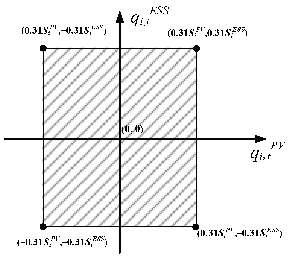
The reactive power of PV power stations and ESSs is expressed as:
q i , t P V & E S S = q i , t P V + q i , t E S S
From the graphical representation in Figure 3, the range of values for q i , t P V & E S S is as follows:
0 . 31 ( S i P V + S i E S S ) q i , t P V & E S S 0 . 31 ( S i P V + S i E S S )
Based on Equations (A7) and (A8), the feasible region of ( q i N B S U , q i P V & E S S ) is plotted on a Cartesian coordinate system, as depicted by the shaded region in Figure A2.
Figure A2. The feasible region of ( q i N B S U , q i P V & E S S ) .
Energies 18 02215 g0a2
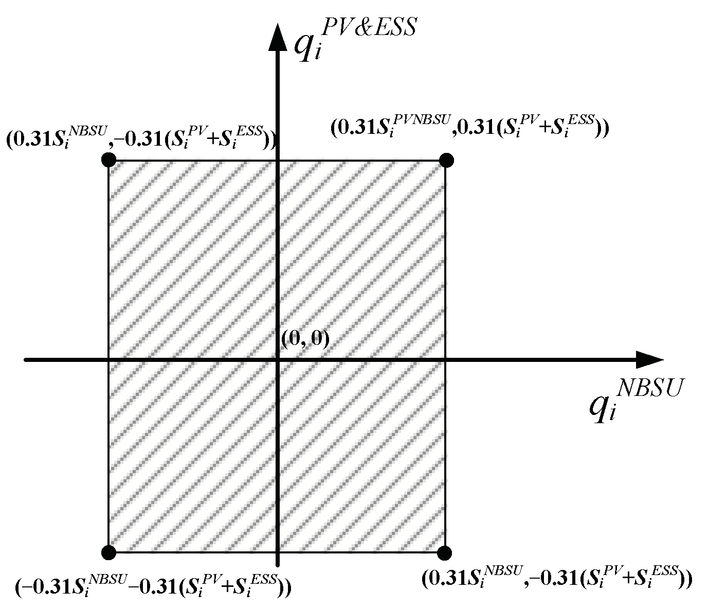
The equation for the net reactive power of LA i at time t is:
q i , t = q i , t P V & E S S + q i , t N B S U q i , t L
From the graphical representation in Figure A2, the range of values for q i , t , which is equivalent to Equation (13a), derived using graphical methods is as follows:
0 . 31 ( S i P V + S i E S S + S i N B S U ) q i , t + q i , t L 0 . 31 ( S i P V + S i E S S + S i N B S U )

Appendix A.2. The Feasible Region of p i , t

  • The aggregated generation of PV power stations
When B = 2, the active power of the PV power stations is expressed as:
p i , t P V = p i , t , 1 P V + p i , t , 2 P V
p i , t , 1 P V and p i , t , 2 P V satisfy Equation (15), and given that 2 S i , b P V ± q i , t , b P V ( 2 0.31 ) S i , b P V > S i , b P V   X i , t 1 ζ i , t , b P V S i , b P V , the range of values for p i , t P V derived using graphical methods is as follows:
0 p i , t P V X i , t 1 ( ζ i , t , 1 P V S i , 1 P V + ζ i , t , 2 P V S i , 2 P V )
Considering Equations (2) and (5), Equation (A13) is equivalent to Equation (13c).
When B > 2, the active power of the PV power stations is expressed as:
p i , t P V = b = 1 B 1 p i , t , b P V + p i , t , B P V
The condition for b = 1 B 1 p i , t , b P V is as follows:
0 b = 1 B 1 p i , t , b P V X i , t 1 b = 1 B 1 ζ i , t , b P V S i , b P V
When p i , t , B P V satisfies Equation (15), and given that 2 S i , b P V ± q i , t , b P V ( 2 0.31 ) S i , b P V > S i , b P V X i , t 1 ζ i , t , b P V S i , b P V , the range of values for p i , t P V , which is equivalent to Equation (13c) in light of Equations (2) and (5), derived using graphical methods is as follows:
0 p i , t P V X i , t 1 b = 1 B ζ i , t , b P V S i , b P V
  • The aggregated generation of ESSs
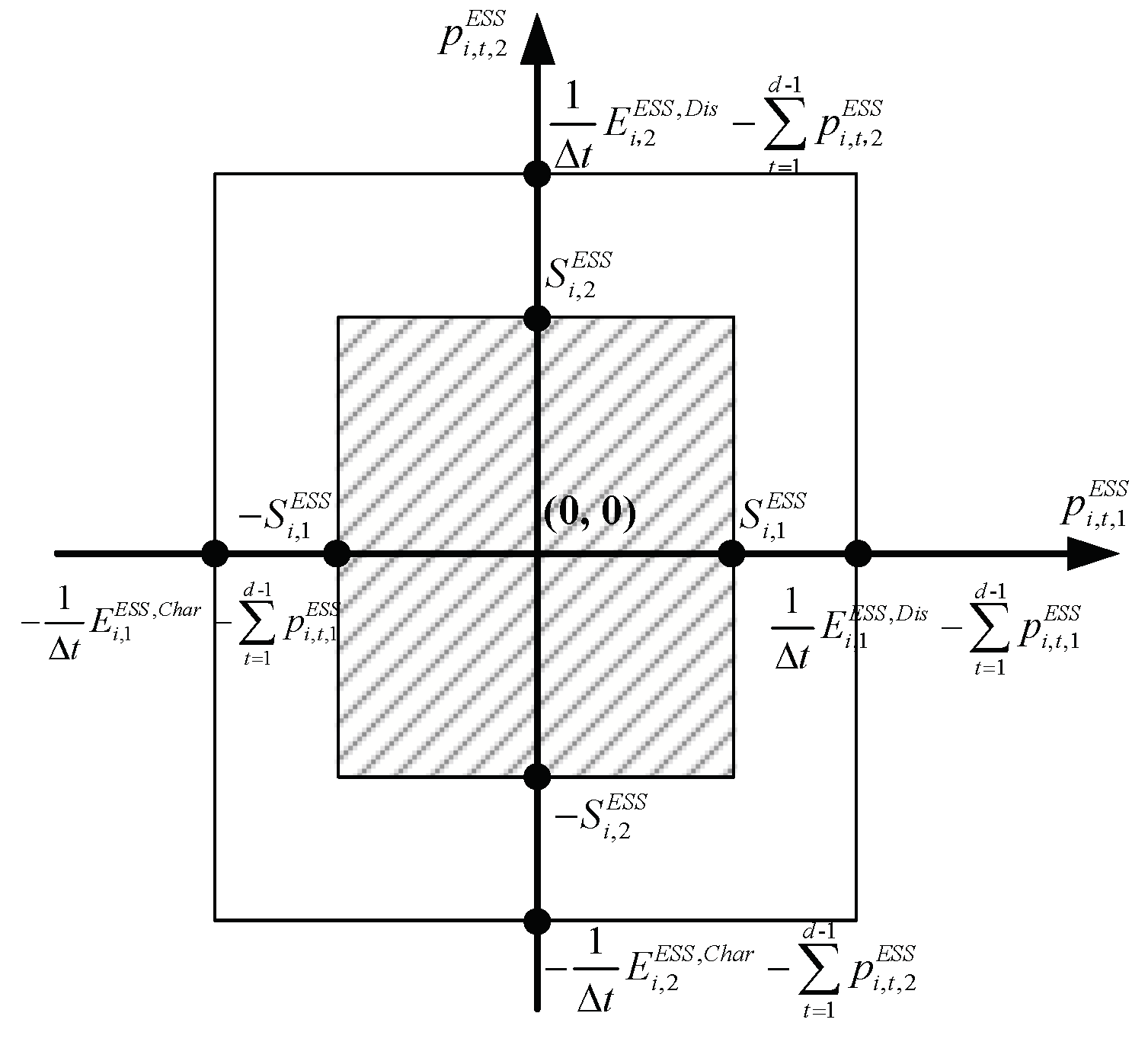
When C = 2, the active power of the ESSs is expressed as:
p i , t E S S = p i , t , 1 E S S + p i , t , 2 E S S
Using Equation (16), the feasible region of ( p i , t , 1 E S S , p i , t , 2 E S S ) is plotted on a Cartesian coordinate system, shown as the shaded area in Figure A3. As t increases, 1 Δ t E i , 1 E S S , D i s t = 1 d - 1 p i , t , 1 E S S and 1 Δ t E i , 1 E S S , C h a r + t = 1 d - 1 p i , t , 1 E S S may decrease to values falling within the range of S i , 1 E S S , while 1 Δ t E i , 2 E S S , D i s t = 1 d - 1 p i , t , 2 E S S and 1 Δ t E i , 2 E S S , C h a r + t = 1 d - 1 p i , t , 2 E S S may be reduced to values within the range of S i , 2 E S S .
Figure A3. The feasible region of ( p i , t , 1 E S S , p i , t , 2 E S S ) .
Energies 18 02215 g0a3
Based on the graphical representation in Figure A1, the range of values for p i , t E S S derived using graphical methods is as follows:
p i , t , 1 E S S , min + p i , t , 2 E S S , min p i , t E S S p i , t , 1 E S S , max + p i , t , 2 E S S , max
where p i , t , 1 E S S , max = min S i , 1 E S S , 1 Δ t E i , 1 E S S , D i s t = 1 d - 1 p i , t , 1 E S S , p i , t , 1 E S S , min = max S i , 1 E S S , 1 Δ t E i , 1 E S S , C h a r t = 1 d - 1 p i , t , 1 E S S , p i , t , 2 E S S , max = min S i , 2 E S S , 1 Δ t E i , 2 E S S , D i s t = 1 d - 1 p i , t , 2 E S S , and p i , t , 2 E S S , min = max S i , 2 E S S , 1 Δ t E i , 2 E S S , C h a r t = 1 d - 1 p i , t , 2 E S S .
When we linearize Equation (A18), we obtain:
min { S i , 1 E S S , S i , 2 E S S } p i , t E S S min { S i , 1 E S S , S i , 2 E S S }
E i E S S , C h a r Δ t t = 1 d p i , t E S S E i E S S , D i s 1 d T
Considering Equations (3), (4) and (8), Equations (A19) and (A20) are equivalent to Equations (13d) and (13e). After linearization in Equations (A19) and (A20), the ESSs’ power capacities decrease, but their overall energy capacity remains unaffected.
When C > 2, the active power of the ESSs is expressed as:
p i , t E S S = c = 1 C 1 p i , t , c E S S + p i , t , C E S S
Similarly, it can be derived that the range of values for p i , t E S S is as follows:
p i , t , C E S S , min + p i , t , 1 ~ ( C - 1 ) E S S , min p i , t E S S p i , t , C E S S , max + p i , t , 1 ~ ( C - 1 ) E S S , max
where p i , t , C E S S , max = min { S i , C E S S , 1 Δ t E i , C E S S , D i s t = 1 d - 1 p i , t , C E S S } , p i , t , 1 ~ ( C - 1 ) E S S , max = min { S i , 1 E S S , S i , 2 E S S , , S i , C 1 E S S , 1 Δ t c = 1 C - 1 E i , c E S S , D i s c = 1 C - 1 t = 1 d - 1 p i , t , C E S S } , p i , t , 1 ~ ( C - 1 ) E S S , min = max { S i , 1 E S S , S i , 2 E S S , , S i , C 1 E S S , 1 Δ t c = 1 C - 1 E i , c E S S , C h a r c = 1 C - 1 t = 1 d - 1 p i , t , C E S S } , and p i , t , C E S S , min = max { S i , C E S S , 1 Δ t E i , C E S S , C h a r t = 1 d - 1 p i , t , C E S S } .
When we linearize Equation (A22), we obtain:
min { S i , 1 E S S , S i , 2 E S S , , S i , C E S S } p i , t E S S min { S i , 1 E S S , S i , 2 E S S , , S i , C E S S }
c = 1 C E i , c E S S , C h a r Δ t t = 1 d c = 1 C p i , t , c E S S c = 1 C E i , C E S S , D i s 1 d T
Considering Equations (3), (4) and (8), Equations (A23) and (A24) are equivalent to Equations (13d) and (1e). After linearization in Equations (A23) and (A24), the ESSs’ power capacities decrease, but their overall energy capacity remains unaffected.
  • The aggregated generation of NBSUs
When E = 2, the active power of the ESSs is expressed as:
p i , t N B S U = p i , t , 1 N B S U + p i , t , 2 N B S U
NBSUs start operating and producing energy simultaneously, maintaining μ i , t , e N B S U = μ i , t N B S U and φ i , t , e N B S U = φ i , t N B S U for dimensionality reduction. For various values of μ i , t N B S U and φ i , t N B S U , the range of p i , t N B S U is presented in Table A1 and Table A2.
Table A1. Upper limit change table for p i , t N B S U (E = 2).
μ i , t N B S U φ i , t N B S U p i , t , 1 N B S U , m a x p i , t , 2 N B S U , m a x
0000
10 p i , 1 N B S U , i n p i , 2 N B S U , i n
11 min { S i , 1 N B S U , p i , t 1 , 1 N B S U + p i , 1 N B S U , u p } min { S i , 2 N B S U , p i , t 1 , 2 N B S U + p i , 2 N B S U , u p }
Table A2. Lower limit change table for p i , t N B S U (E = 2).
μ i , t N B S U φ i , t N B S U p i , t , 1 N B S U , m i n p i , t , 2 N B S U , m i n
0000
10 p i , 1 N B S U , i n p i , 2 N B S U , i n
11 max { 0 , p i , t 1 , 1 N B S U p i , 1 N B S U , d o w n } max { 0 , p i , t 1 , 2 N B S U p i , 2 N B S U , d o w n }
The range of values for variable p i , t N B S U based on Equations (9)–(12) and Table A1 and Table A2 are defined as follows:
0 p i , t N B S U ( φ i , t N B S U μ i , t N B S U ) p i N B S U , i n φ i , t N B S U ( S i , 1 N B S U + S i , 2 N B S U )
φ i , t 1 N B S U 1 M p i N B S U , d o w n p i , t N B S U p i , t 1 N B S U 1 φ i , t 1 N B S U M + p i N B S U , u p
Equation (A26) is equal to Equation (13i), and Equation (A27) is equal to Equation (13j).
When E > 2, the active power of the ESSs is expressed as:
p i , t N B S U = e = 1 E 1 p i , t , e N B S U + p i , t , E N B S U
The NBSUs start operating and producing energy simultaneously, maintaining μ i , t , e N B S U = μ i , t N B S U and φ i , t , e N B S U = φ i , t N B S U for dimensionality reduction. For various values of μ i , t N B S U and φ i , t N B S U , the range of p i , t N B S U is presented in Table A3 and Table A4.
Table A3. Upper limit change table for p i , t N B S U (E > 2).
μ i , t N B S U φ i , t N B S U e = 1 E 1 p i , t , e N B S U p i , t , E N B S U , m a x
0000
10 p i , 1 ~ ( E 1 ) N B S U , i n p i , E N B S U , i n
11 min { S i , 1 ~ E - 1 N B S U , e = 1 E 1 p i , t - 1 , e N B S U + p i , 1 ~ E 1 N B S U , u p } min { S i , E N B S U , p i , t 1 , E N B S U + p i , E N B S U , u p }
Table A4. Lower limit change table for p i , t N B S U (E > 2).
μ i , t N B S U φ i , t N B S U e = 1 E 1 p i , t , e N B S U p i , t , E N B S U , m i n
0000
10 p i , 1 ~ ( E 1 ) N B S U , i n p i , E N B S U , i n
11 max { 0 , e = 1 E 1 p i , t - 1 , e N B S U p i , 1 ~ ( E 1 ) N B S U , d o w n } max { 0 , p i , t 1 , E N B S U p i , E N B S U , d o w n }
Here, p i , 1 ~ ( E 1 ) N B S U , i n = ( e = 1 E - 1 T i , e N B S U p i , e N B S U , i n ) / T i N B S U , p i , 1 ~ ( E 1 ) N B S U , u p = min { p i , 1 N B S U , u p , p i , 2 N B S U , u p , , p i , E 1 N B S U , u p } , and p i , 1 ~ ( E 1 ) N B S U , d o w n = min { p i , 1 N B S U , d o w n , p i , 2 N B S U , d o w n , , p i , E 1 N B S U , d o w n } .
The range of values for variable p i , t N B S U based on Equations (9)–(12) and Table A3 and Table A4 are defined as follows:
0 p i , t N B S U ( φ i , t N B S U μ i , t N B S U ) p i N B S U , i n φ i , t N B S U e = 1 E S i , e N B S U
φ i , t 1 N B S U 1 M p i N B S U , d o w n p i , t N B S U p i , t 1 N B S U 1 φ i , t 1 N B S U M + p i N B S U , u p
Equation (A29) is equal to Equation (13i), and Equation (A30) is equal to Equation (13j).
In summary, Equation (13) is a sufficient condition for the set of Equations (14)~(17), which means Ω D C , n e t Ω L A , n e t and ensuring that all PSC-based net power plans are feasible for DG within LAs.

References

  1. U.S. Department of Energy. Hurricane Fiona|Update #1; U.S. Department of Energy: Washington, DC, USA, 2022. Available online: http://www.energy.gov/sites/default/files/2022-09/TLP-CLEAR_Fiona_DOE%20Situation%20Update_1.pdf (accessed on 19 September 2022).
  2. Aoyu, L.; Jian, Z.; Yong, M.; Linag, T.; Hong, W.; Jialu, L. Analysis and Lessons of the Blackout in Chinese Taiwan Power Grid on March 3, 2022. South. Power Syst. Technol. 2022, 16, 90–97. [Google Scholar]
  3. National Power Control Center. Power Breakdown in the Country on 23 January 2023; National Power Control Center: Islamabad, Pakistan, 2023. [Google Scholar]
  4. Schmitt, K.; Bhatta, R.; Chamana, M.; Murshed, M.; Osman, I.; Bayne, S.; Canha, L. A Review on Active Customers’ Participation in Smart Grids. J. Mod. Power Syst. Clean Energy 2023, 11, 3–16. [Google Scholar] [CrossRef]
  5. Nazemi, M.; Dehghanian, P.; Alhazmi, M.; Darestani, Y. Resilient Operation of Electric Power Distribution Grids Under Progressive Wildfires. IEEE Trans. Ind. Appl. 2022, 58, 1632–1643. [Google Scholar] [CrossRef]
  6. Diahovchenko, I.M.; Kandaperumal, G.; Srivastava, A.K. Enabling resiliency using microgrids with dynamic boundaries. Electr. Power Syst. Res. 2023, 221, 109460. [Google Scholar] [CrossRef]
  7. Sadnan, R.; Poudel, S.; Dubey, A.; Schneider, K.P. Layered Coordination Architecture for Resilient Restoration of Power Distribution Systems. IEEE Trans. Ind. Inform. 2023, 19, 6069–6080. [Google Scholar] [CrossRef]
  8. Kalantari, A.; Restrepo, J.F.; Galiana, F.D. Security-constrained unit commitment with uncertain wind generation: The loadability set approach. IEEE Trans. Power Syst. 2013, 28, 1787–1796. [Google Scholar] [CrossRef]
  9. Zhao, L.; Zhang, W.; Hao, H.; Karanjit, K. A geometric approach to aggregate flexibility modeling of thermostatically controlled loads. IEEE Trans. Power Syst. 2017, 32, 4721–4731. [Google Scholar] [CrossRef]
  10. Ardakani, A.J.; Bouffard, F. Identification of umbrella constraints in DC-based security-constrained optimal power flow. IEEE Trans. Power Syst. 2013, 28, 3924–3934. [Google Scholar] [CrossRef]
  11. Abiri-Jahromi, A.; Bouffard, F. On the loadability sets of power systems—Part II: Minimal representations. IEEE Trans. Power Syst. 2017, 32, 146–156. [Google Scholar] [CrossRef]
  12. Ma, Z.; Zhou, Y.; Zheng, Y.; Yang, L.; Wei, Z. Distributed Robust Optimal Dispatch of Regional Integrated Energy Systems Based on ADMM Algorithm with Adaptive Step Size. J. Mod. Power Syst. Clean Energy 2024, 12, 852–862. [Google Scholar] [CrossRef]
  13. Xiao, J.; Li, F.; Gu, W.; Wang, C.; Zhang, P. Total supply capability and its extended indices for distribution systems: Definition model calculation and applications. IET Gener. Transm. Distrib. 2011, 5, 869–876. [Google Scholar] [CrossRef]
  14. Xiao, J.; Li, X.; Gu, W.; Li, F.; Wang, C. Model of distribution system total supply capability considering feeder and substation transformer contingencies. Int. J. Electr. Power Energy Syst. 2015, 65, 419–424. [Google Scholar] [CrossRef]
  15. Ding, T.; Li, C.; Zhao, C.; Wang, M. Total supply capability considering distribution network reconfiguration under N-k transformer contingency and the decomposition method. IET Gener. Transm. Distrib. 2017, 11, 1212–1222. [Google Scholar] [CrossRef]
  16. Chen, K.; Wu, W.; Zhang, B.; Djokic, S.; Harrision, G. A Method to Evaluate Total Supply Capability of Distribution Systems Considering Network Reconfiguration and Daily Load Curves. IEEE Trans. Power Syst. 2016, 31, 2096–2104. [Google Scholar] [CrossRef]
  17. Xiao, J.; Liu, S.; Li, Z.; Li, F. Load ability formulation and calculation for interconnected distribution systems considering N-1 security. Int. J. Electr. Power Energy Syst. 2016, 77, 70–76. [Google Scholar] [CrossRef]
  18. Xu, Z.; Liu, H.; Sun, H.; Ge, S.; Wang, C. Power supply capability evaluation of distribution systems with distributed generations under differentiated reliability constraints. Int. J. Electr. Power Energy Syst. 2022, 134, 107344. [Google Scholar] [CrossRef]
  19. Luo, F.; Wang, C.; Xiao, J.; Ge, S. Rapid evaluation method for power supply capability of urban distribution system based on N-1 contingency analysis of main-transformers. Int. J. Electr. Power Energy Syst. 2010, 32, 1063–1068. [Google Scholar] [CrossRef]
  20. Silva, J.; Sumaili, J.; Bessa, R.J.; Seca, L.; Matos, M.A.; Miranda, V.; Caujolle, M.; Goncer, B.; Sebastian-Viana, M. Estimating the active and reactive power flexibility area at the TSO-DSO interface. IEEE Trans. Power Syst. 2018, 33, 4741–4750. [Google Scholar] [CrossRef]
  21. Chen, Y.; Weijia, G.; Junting, L.; Li, Z.; Xiaofeng, D.; Qiong, Z.; Junpeng, Z. Linear Programming Method of Dynamic Fault Restoration for Distribution Network Considering Balanced Node. In Proceedings of the 2023 IEEE/IAS Industrial and Commercial Power System Asia (I&CPS Asia), Chongqing, China, 7–9 July 2023; pp. 1088–1093. [Google Scholar] [CrossRef]
  22. Xiao, J.; Wang, C.; She, B.; FX, L.; ZY, B.; XS, Z. Total supply and accommodation capability curves for active distribution networks: Concept and model. Int. J. Electr. Power Energy Syst. 2021, 133, 107279. [Google Scholar] [CrossRef]
  23. Xiao, J.; Cai, Z.W.; Liang, Z.Y.; She, B.X. Mathematical model and mechanism of TSC curve for distribution networks. Int. J. Electr. Power Energy Syst. 2022, 137, 107812. [Google Scholar] [CrossRef]
  24. Xiao, J.; Zhang, T.; Zu, G.; Li, F.X.; Wang, C.S. TSC-Based Method to Enhance Asset Utilization of Interconnected Distribution Systems. IEEE Trans. Smart Grid 2018, 9, 1718–1727. [Google Scholar] [CrossRef]
  25. Zafeiropoulou, M.; Sijakovic, N.; Zarkovic, M.; Ristic, V.; Terzic, A.; Makrygiorgou, D.; Zoulias, E.; Vita, V.; Maris, T.I.; Fotis, G. Development and Implementation of a Flexibility Platform for Active System Management at Both Transmission and Distribution Level in Greece. Appl. Sci. 2023, 13, 11248. [Google Scholar] [CrossRef]
  26. IEC 60870-5-104; Telecontrol Equipment and Systems—Part 5-104: Transmission Protocols—Network Access for IEC 60870-5-101 Using Standard Transport Profiles. 2nd ed. International Electrotechnical Commission: Geneva, Switzerland, 2006.
Figure 1. The distribution system configuration.
Energies 18 02215 g001
Figure 2. The information-sharing framework.
Energies 18 02215 g002
Figure 3. A 10 kV urban 45-bus distribution network test system.
Energies 18 02215 g003
Figure 4. The recovery scheme of the network topology (4:00–9:00).
Energies 18 02215 g004
Figure 5. The recovery scheme of generation (4:00–9:00). Note: In Figure 5, ‘ESS27’ means the ESS in LA 27.
Energies 18 02215 g005
Figure 6. The recovery scheme of the network topology (10:00–15:00).
Energies 18 02215 g006
Figure 7. The recovery scheme of generation (10:00–15:00).
Energies 18 02215 g007
Figure 8. The static scheme.
Energies 18 02215 g008
Table 1. Hardware configuration of LAs.
The Components of a LAConfiguration
GPU running1.2 GHz (Cortex-A71)
Internal memory150 MB
Storage4 GB
Operating systemArmv71 GNU/Linux
Table 2. Details of the PV power stations.
Bus No.Voltage LevelInstalled Capacity (kW)
2010 kV260
2310 kV260
28380/220 V2800
3810 kV1000
Table 3. Details of the ESSs.
Bus No. E i , c E S S , D i s (kWh) E i , c E S S , C h a r (kW) S i , c E S S (kW)
25145050500
27232080800
37145050200
Table 4. Details of the NBSUs.
Bus No. S i , e N B S U (kW) p i , e N B S U , i n (kW) p i , e N B S U , u p (kW/h) p i , e N B S U , d o w n (kW/h) T i N B S U (h)
363606.43603600.5
44800.880800.5
454007.24004000.5
Table 5. Details of the lines.
Start BusTermination NodeTotal Line Length (m)Line ModelConductor Section (mm2)
12420YJV22-8.7/15-3*300300
23226JKLYJ-10/185185
34138JKLYJ-10/185185
320130JKLYJ-10/185185
2021180JKLYJ-10/185185
2122170JKLYJ-10/185185
2223280JKLYJ-10/185185
45145JKLYJ-10/185185
56——————
67136JKLYJ-10/185185
78150JKLYJ-10/185185
89162JKLYJ-10/185185
910——————
1011700JKLYJ-10/185185
1112160JKLYJ-10/185185
1213153JKLYJ-10/185185
1314——————
1415102JKLYJ-10/185185
1516505JKLYJ-10/185185
1617——————
1718105JKLYJ-10/185185
1819170YJV22-8.7/15-3*300300
124196YJV22-8.7/15-3*300300
2425148YJV22-8.7/15-3*300300
2426120YJV22-8.7/15-3*300300
242792YJV22-8.7/15-3*300300
2428116YJV22-8.7/15-3*300300
2429370YJV22-8.7/15-3*300300
2930150YJV22-8.7/15-3*300300
2931375YJV22-8.7/15-3*300300
2932150YJV22-8.7/15-3*300300
3233802YJV22-8.7/15-3*300300
3234120YJV22-8.7/15-3*300300
3235806YJV22-8.7/15-3*300300
3536132JKLYJ-10/185185
3637150JKLYJ-10/185185
3738132JKLYJ-10/185185
3839——————
3940180JKLYJ-10/185185
4041233JKLYJ-10/185185
4142160JKLYJ-10/185185
4243——————
4344155JKLYJ-10/185185
Note: In Table 5, ‘3*300’ means ‘three conductors, with a single section of 300 mm2’.
Disclaimer/Publisher’s Note: The statements, opinions and data contained in all publications are solely those of the individual author(s) and contributor(s) and not of MDPI and/or the editor(s). MDPI and/or the editor(s) disclaim responsibility for any injury to people or property resulting from any ideas, methods, instructions or products referred to in the content.

