Automated Detection Method for Bolt Detachment of Wind Turbines in Low-Light Scenarios

Abstract

Tower bolts play a crucial role as connecting components in wind turbines and are of great interest for health monitoring systems. Non-contact monitoring techniques offer superior efficiency, convenience, and intelligence compared to contact-based methods. However, the precision and robustness of the non-contact monitoring process are significantly impacted by suboptimal lighting conditions within the wind turbine tower. To address this problem, this article proposes an automated detection method for the bolt detachment of wind turbines in low-light scenarios. The approach leverages the deep convolutional generative adversarial network (DCGAN) to expand and augment the small-sample bolt dataset. Transfer learning is then applied to train the Zero-DCE++ low-light enhancement model and the bolt defect detection model, with the experimental verification of the proposed method’s effectiveness. The results reveal that the deep convolutional generative adversarial network can generate realistic bolt images, thereby improving the quantity and quality of the dataset. Additionally, the Zero-DCE++ light enhancement model significantly increases the mean brightness of low-light images, resulting in a decrease in the error rate of defect detection from 31.08% to 2.36%. In addition, the model’s detection performance is affected by shooting angles and distances. Maintaining a shooting distance within 1.6 m and a shooting angle within 20° improves the reliability of the detection results.

1. Introduction

The tower, being the most vital load-bearing element in wind turbines, is typically constructed as a steel structure for commercially megawatt turbines. Bolted connections are widely utilized in wind turbine towers due to their advantages in construction convenience [1]. However, wind turbines, particularly those located offshore, face highly intricate load conditions. Given their pivotal role in connecting the tower sections, bolts are susceptible to fatigue fractures, resulting in a substantial reduction in the operational efficiency of wind turbines and potentially leading to catastrophic accidents, including structural collapse [2,3]. Manual inspection, the main approach for detecting bolt defect in wind turbines, is marred by low detection efficiency, high latency, and high risk, with the detection results relying on the experience of inspectors. Therefore, developing more intelligent and efficient bolt defect detection methods is an urgent hot issue.

Extensive research has been conducted on health monitoring techniques for tower bolts and contact-based methods remain the most commonly employed approach. Nevertheless, the widespread use of this method is hindered by the need to install a large number of costly sensors on the structure, as well as the complexities associated with data analysis. Additionally, the time-dependent characteristics of the detection results further limit its applicability in bolt arrays. A large number of domestic and international scholars have utilized various sensing technologies to detect bolt defect. Strain sensors [4], optical fiber sensors [5], piezoelectric sensors [6], and acoustic sensors [7] are deployed on structures, and diverse data analysis methods are employed to assess the health status of bolts. Due to the nonlinearity and uncertainty of sensor signals, accurately assessing the state of bolts is a challenge. Hence, many scholars have proposed more advanced analysis methods to handle complex sensor signals [8,9,10], achieving certain progress at the theoretical level.

Non-contact monitoring techniques have gained widespread application in wind turbine systems due to the rapid advancement of computer technology. Compared to contact-based monitoring techniques, non-contact methods offer advantages such as cost-effectiveness, high efficiency, and increased intelligence. Early studies have demonstrated the feasibility of using machine learning and image processing technologies for bolt defect detection, such as support vector machines [11], edge detection [12], threshold segmentation [13], and Hough line transformation [14]. However, these methods struggle to extract effective features from complex environments and backgrounds. In contrast, deep learning methods exhibit efficient feature extraction and analysis capabilities, making it possible to accurately detect defects in complex structures. Some scholars have employed region-based convolutional neural networks such as R-CNN [15], Fast-RCNN [16], Faster-RCNN [17], and Mask-RCNN [18] to detect structural bolt defects with high precision, but they have certain limitations in detection speed. To explore the feasibility of the online monitoring of structural bolt defect, many scholars have utilized single-stage algorithms such as you only look once (YOLO) [19,20,21,22], Retina-Net [23], and single-shot multibox detector (SSD) [24] to perform regression classification on structural bolt defect.

These methods are entirely dependent on large-image datasets. The quantity and diversity of datasets determine the accuracy and robustness of various detectors. Autonomously collecting and constructing large bolt image datasets is a difficult task. Therefore, many scholars use conventional transformations and deep learning methods to augment small sample datasets [25,26]. Generative adversarial networks [25] can learn the feature distribution of real image datasets and generate an infinite number of high-quality realistic images with similar feature distributions, which can be used for the efficient augmentation of small sample datasets and has been widely applied in many fields such as medical [27], transportation [28], energy [29], and agriculture [30].

Currently, most bolt defect detection models based on deep learning have achieved remarkable results in normal lighting environments [31,32,33]. However, due to insufficient lighting sources in the vicinity of the bolts, especially flange bolts, wind turbine structures often experience low-light environments. This leads to a significant reduction in the accuracy and robustness of bolt defect detection models, making it difficult to ensure the service safety of bolts in wind turbine structures. Using deep learning methods to enhance low-light images is a feasible solution, mainly including supervised learning and unsupervised learning. Supervised learning methods enhance images by learning the mapping relationship between low-light images and normal-light images, such as LightenNet [34], Kind [35], and Kind++ [36]. These methods require a large amount of paired image data for training and have high dependence on and requirements for datasets, limiting their application in practical engineering. Therefore, unsupervised learning methods have emerged. The EnlightGAN [37] network generates high-brightness images by learning image feature distributions, but it has drawbacks such as unnatural generated images and a large number of network parameters, so it is less used in practical engineering. To improve model inference speed and reduce computational costs, Ma [38] and others proposed an unsupervised learning framework for self-calibrated illumination (SCI), which can achieve network cascading and weight sharing. Inspired by the brightness adjustment curves in image editing software, Guo [39] and others proposed a low-light image enhancement algorithm Zero-DCE based on brightening curves and convolutional neural networks, realizing the remapping of low-light pixels to high-brightness pixels. To balance model performance and computational costs, Li [40] and others optimized Zero-DCE and proposed a lightweight version, Zero-DCE++.

In summary, contact-based inspection methods such as vibration analysis [41,42,43] and acoustic sensing [44,45,46,47] are widely adopted techniques for bolt defect identification, enabling high-precision defect diagnosis. However, they face challenges in cost, sensitivity to environmental noise, real-time performance, and scalability for large bolt arrays. Vision-based bolt defect detection, categorized as a non-contact inspection method [48,49], demonstrates significant improvements in cost-efficiency and real-time capability compared to contact-based approaches. Nevertheless, its accuracy and robustness are substantially compromised under low-light environments, particularly in offshore wind turbines with submerged tower sections. To address these limitations, this paper proposes an automated bolt defect detection method for wind turbines that integrates an unsupervised low-light enhancement model (Zero-DCE++) and a lightweight object detection model. This approach effectively overcomes the critical limitations of existing methods, such as dependency on illumination conditions and insufficient robustness, thereby the advancing reliability in low-light scenarios. The three novelties of this paper are as follows: (1) using a deep convolutional generative adversarial network to perform the generative expansion and augmentation of bolt image datasets to enrich the diversity of the dataset; (2) using the unsupervised low-light enhancement algorithm Zero-DCE++ to achieve the rapid enhancement of wind turbine bolt images under low-light conditions, and the detection accuracy of the bolt defect is significantly improved after enhancement; (3) selecting a lightweight target detection algorithm. After integrating the light enhancement algorithm, it can realize real-time monitoring of the connection status of bolts in wind turbine structures and improve the level of automation.

2. Methods

2.1. Overview

The framework of the automated detection method for bolt detachment defect is depicted in Figure 1. It can be segmented into the following steps:

(1)

Dataset preparation phase: Acquire the bolt image dataset through multiple channels. Construct and train a deep convolutional generative adversarial network to deeply expand and augment the bolt images. The unlabeled images after deep expansion serve as dataset 1, while the labeled images are added as dataset 2. Both types are utilized in the subsequent network training process.

(2)

Model training stage: Firstly, construct the low-light enhancement model Zero-DCE++ and train it using dataset 1. Secondly, build the bolt defect detection model and train it with dataset 2.

(3)

Disease identification phase: Based on the YUV color space method, separate the brightness (Y) and chrominance (UV) features of the collected image awaiting detection. Calculate the feature value of the brightness component to categorize the image into low-light and normal-light types. For low-light images, conduct image brightness enhancement processing first, and then input them along with normal-light images into the bolt detachment defect model to accomplish the automated detection of bolt defect.

(4)

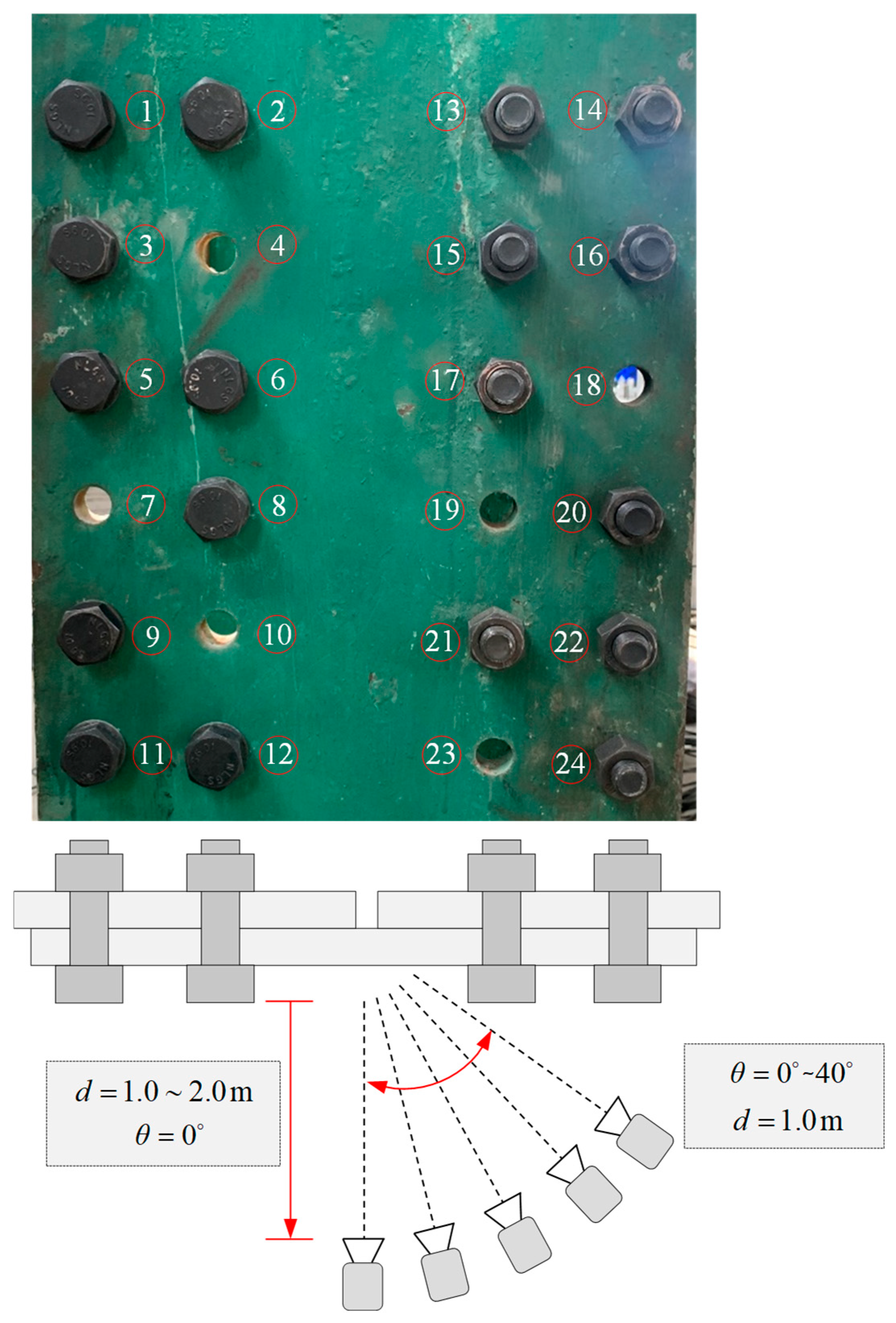
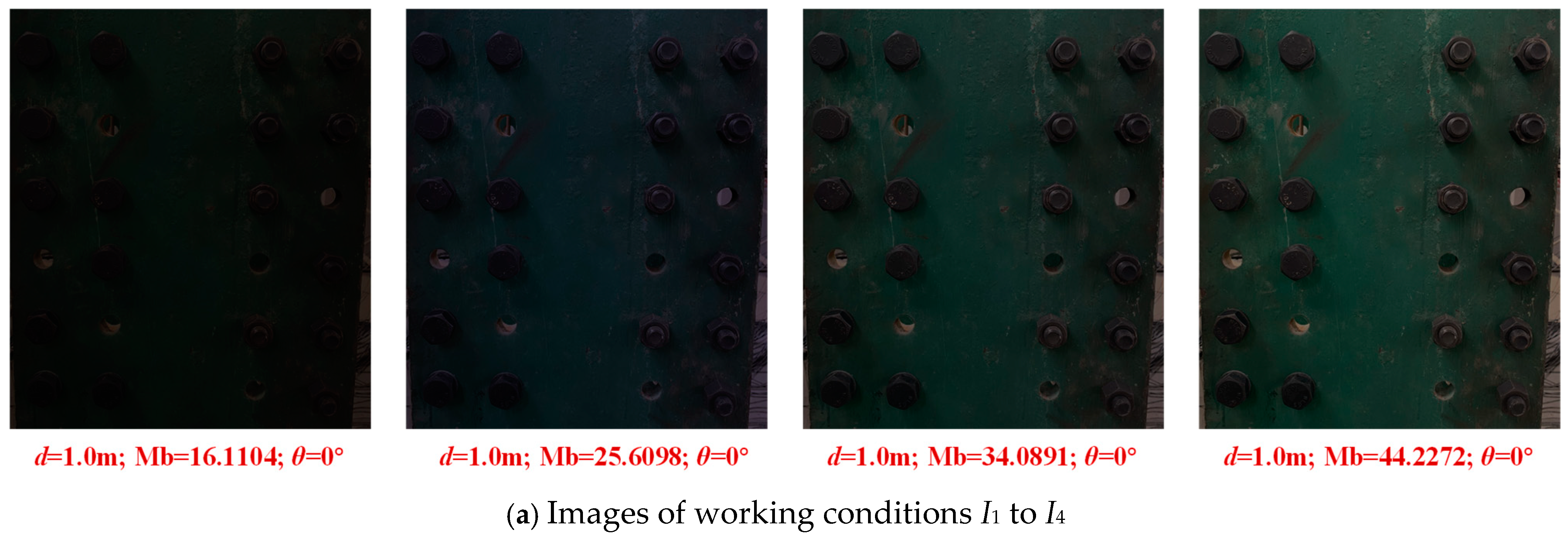
Method effectiveness analysis: Verify the effectiveness of the proposed method via experiments (in Changsha, Hunan Province, China). Analyze the impact of the shooting angle, distance, and light intensity on model performance by altering different imaging conditions.

In order to accomplish its objectives, this study employed various key methodologies. These encompassed the utilization of DCGAN [50] to augment the dataset, enhancing low-light images through Zero-DCE++ [40], and detecting bolt detachment defects using object detection algorithms. Detailed descriptions of these methodologies are provided in Section 2.2, Section 2.3 and Section 2.4.

2.2. Data Generation Augmentation and Evaluation

2.2.1. Deep Convolutional Generative Adversarial Network (DCGAN)

In actual wind turbines, the positions, functions, and environments of bolt connections exhibit diversity. Moreover, following bolt fatigue fracture and detachment, the connection performance is significantly degraded, presenting a severe threat to the structural safety of wind turbines. To enhance the robustness and generalization ability of the detection model for bolt detachment defect in wind turbines, it is proposed to employ the DCGAN to deeply expand the small collected sample dataset and increase the diversity thereof.

DCGAN consists of two networks: generator (G) and discriminator (D). A convolutional neural network is added to the generative adversarial network for feature extraction. The network structure diagram of DCGAN is depicted in Figure 2. First, random noise z that obeys a specific distribution is input into the generator. After a series of deconvolution operations, the image gradually enlarges, and finally a generated pseudo-bolt image is output. The generator learns the data distribution characteristics of real bolt images to ensure that the generated pseudo-bolt image and the real bolt image follow as closely as possible the same probability distribution. Secondly, the generated pseudo-bolt image and the real bolt image are input into the discriminator. After a series of convolution operations, the image gradually shrinks, and finally, a probability is output to determine the authenticity of the input image. The discriminator continuously learns to ensure the accurate discrimination of the authenticity of the input image. Finally, the generator and discriminator undergo continuous adversarial training, and the discrimination error is back-propagated to update the network parameters. Eventually, the two reach a Nash equilibrium state. At this time, the probability distribution of the pseudo-image generated by the generator and the real image is identical, and the discriminator has an equal probability of determining whether the input image is true or false. Therefore, the trained generator can be used to generate multiple pseudo-images with similar but not identical feature distributions to the real image to deeply expand the dataset.

To quantify the error in the adversarial training process of DCGAN, the loss functions of the generator and discriminator are constructed, as shown in Equation (1) [50].

$$L_G={\displaystyle \frac{1}{N}}{\displaystyle \sum _{i=1}^N[\ln (1-D(G(z^{(i)})))]}, L_D={\displaystyle \frac{1}{N}}{\displaystyle \sum _{i=1}^N[\ln D(x^{(i)})+\ln (1-D(G(z^{(i)})))]}$$

(1)

where z represents the input random noise, N represents the total number of input images, x represents the real image, G(z) represents the pseudo-image generated by the generator, D(x) represents the probability value evaluated by the discriminator that an image is a real image, D(G(z)) represents the probability value evaluated by the discriminator that an image is a pseudo-image.

In deep learning networks, the prediction accuracy of the network output directly depends on the network parameters. Therefore, in the process of network iterative training, the network parameters need to be continuously updated based on the loss value of the model until the loss value is minimized. At this point, the corresponding model parameters are the optimal parameters. The network output value can be determined by the network input parameters (as in Equation (2)) and the activation function (as in Equation (3)), and compared with the network true value (as in Equation (4)). The optimal parameters of the network are continuously determined through an iterative solution.

$$x=\left(x_1,x_2,\cdots ,x_n\right)$$

(2)

$$\widehat{y}=f(\omega \cdot x+b)=({\widehat{y}}_1,{\widehat{y}}_2,\cdots ,{\widehat{y}}_n)$$

(3)

$$y=\left(y_1,y_2,\cdots ,y_n\right)$$

(4)

where n is the number of samples, f(·) is the activation function, ω is the weight matrix, b is the bias vector.

To accelerate obtaining the optimal parameters when the loss value reaches the minimum, the gradient descent method [51] is commonly used to update the weight and bias parameters of each layer of the network. The calculation is as shown in Equation (5).

$${\omega }_j\to {\omega }_j^{\ast }={\omega }_j-\eta {\displaystyle \frac{\partial L}{\partial {\omega }_j}}, b_j\to b_j^{\ast }=b_j-\eta {\displaystyle \frac{\partial L}{\partial b_j}}$$

(5)

where j represents the jth layer of the network, ω_j and b_j are the weight matrix and bias vector before network update, respectively, η is the learning rate, L is the loss function, which is calculated by Equation (1), ${\omega }_j^{\ast }$ and $b_j^{\ast }$ are the weight matrix and bias vector after the network update, respectively.

2.2.2. Image Similarity Evaluation Metrics

Since the subjective evaluation of image similarity has significant randomness, objective metrics such as mean squared error (MSE), peak signal-to-noise ratio (PSNR), and structural similarity index measure (SSIM) are employed to quantitatively assess image similarity [52].

MSE directly computes the sum of squares of the differences between pixel points of two images, reflecting the absolute error between them, as shown in Equation (6).

$$MSE={\displaystyle \frac{1}{M\times N}}{\displaystyle \sum _{i=1}^M{\displaystyle \sum _{j=1}^N{\left[P(i,j)-R(i,j)\right]}^2}}$$

(6)

where M and N are, respectively, the length and width of the image, P(i, j) and R(i, j) are the pixel values of two different images at point (i, j).

PSNR converts the difference in pixel values in MSE into a difference in decibel values, as shown in Equation (7). The larger its value, the higher the similarity between images.

$$PSNR=10{\log }_{10}{\displaystyle \frac{Q^2}{MSE}}$$

(7)

where Q represents the maximum dynamic range of the image data type. For a specific type of image (8-bit images), it is a constant. Set Q = 255.

SSIM compares the differences in brightness, contrast, and structure between two images, as shown in Equation (8). It is a comprehensive evaluation metric for image quality and has boundedness, that is, SSIM(x,y) ≤ 1. When SSIM(x,y) = 1, the two images are identical.

$$SSIM(x,y)={\displaystyle \frac{(2{\mu }_x{\mu }_y+C_1)(2{\sigma }_{xy}+C_2)}{({\mu }_x^2+{\mu }_y^2+C_1)({\sigma }_x^2+{\sigma }_y^2+C_2)}}$$

(8)

where x and y are two images, μ_x and μ_y are the means of x and y, respectively, σ_xy is the covariance of x and y, σ_x and σ_y are the variances of x and y, respectively, C₁ and C₂ are constants, ensuring numerical stability across brightness and contrast ranges. C₁ = (K₁Q)², C₂ = (K₂Q)². Set K₁ = 0.01 and K₂ = 0.03 [53].

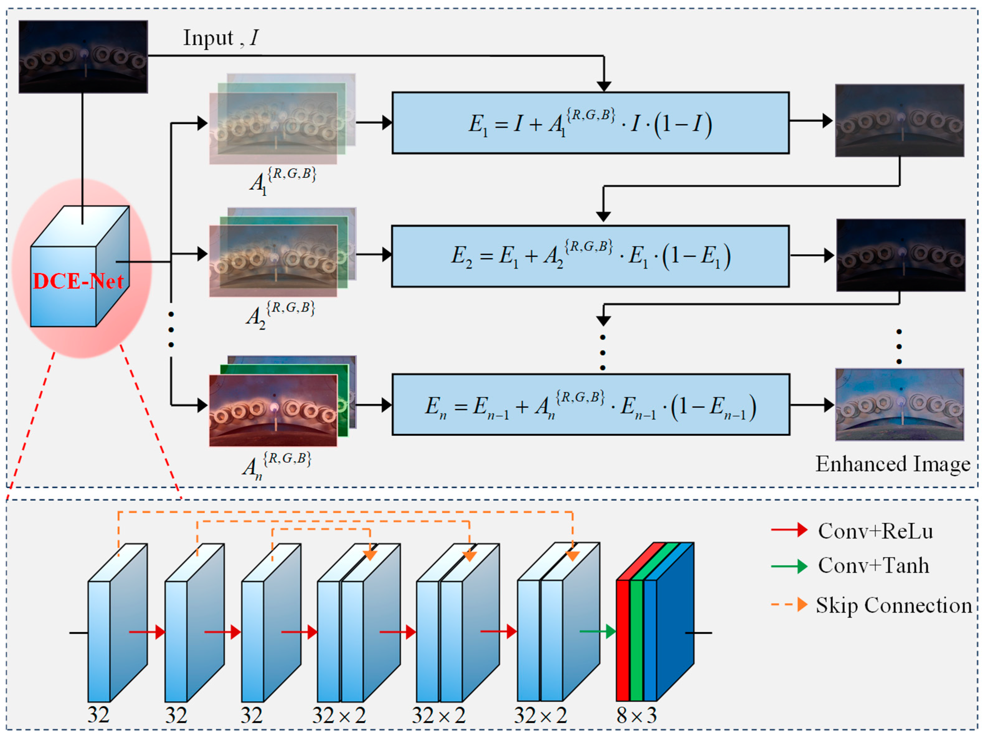
2.3. Low-Light Image Enhancement Algorithm Based on Zero-DCE++

The Zero-DCE++ low-light image enhancement algorithm comprises two components: the light enhancement curve and the deep curve estimation network. The network structure is illustrated in Figure 3.

2.3.1. Light-Enhancement Curve (LE-Curve)

Altering the parameters of the LE-Curve enables the remapping from low-brightness pixels to high-brightness pixels, thereby accomplishing the enhancement of low-light images. The LE-Curve is as presented in Equation (9) [39].

$$E_n\left(x\right)=E_{n-1}\left(x\right)+A_n\left(x\right)\cdot E_{n-1}\left(x\right)\cdot \left[1-E_{n-1}\left(x\right)\right]$$

(9)

where x represents the pixel coordinate of the image, A_n(x) is the LE-Curve parameter to be learned, and E_n(x) denotes the image after light enhancement, and n is the number of iterations.

2.3.2. Deep Curve Estimation Network (DCE-Net)

To obtain the optimal parameters of the LE-Curve, the DCE-Net is employed for iterative training and solution. DCE-Net consists of six hidden layers and one output layer. Each layer performs feature extraction through deep separable convolution and activation functions. Symmetric jump connections are utilized between each hidden layer to achieve the reuse and deep fusion of features between different layers.

2.3.3. Loss Function

The loss function of the Zero-DCE++ model includes four parts: spatial consistency loss L_spa, exposure control loss L_exp, color constancy loss L_col, and illumination smoothness loss L_tva [39]. The total loss function is as shown in Equation (10), where λ₁, λ₂, λ₃, and λ₄ are the corresponding weight coefficients, respectively.

$$L_{total}={\lambda }_1{L}_{spa}+{\lambda }_2{L}_{exp}+{\lambda }_3{L}_{col}+{\lambda }_4{L}_{tva}$$

(10)

L_spa measures the error between adjacent pixels in the local area of the image, as shown in Equation (11), where K is the number of pixels in the local area of the image, Ω(i) the four neighboring regions (top, down, left, right) centered at the region i, and I and Y are the input image and the enhanced image, respectively.

$$L_{spa}={\displaystyle \frac{1}{K}}{\displaystyle \sum _{i=1}^K{\displaystyle {\sum }_{j\in \Omega (i)}{\left(\left|Y_i-Y_j\right|-\left|I_i-I_j\right|\right)}^2}}$$

(11)

L_exp limits the severe polarization of pixels, as shown in Equation (12). where M is the number of pixels in the 16 × 16 area, Y_k is the average brightness value at a certain pixel k, and E is the intermediate brightness value, taken as 0.6.

$$L_{exp}={\displaystyle \frac{1}{M}}{\displaystyle \sum _{k=1}^M\left|Y_k-E\right|}$$

(12)

L_col limits the color deviation between the pixels of the RGB three channels, as shown in Equation (13). where R, G, and B are the red, green, and blue channels of the image, respectively, (p, q) is a random combination of two color channels, and J_p and J_q are the average brightness values of color channels p and q, respectively.

$$L_{col}={\displaystyle {\sum }_{\forall (p,q)\in \epsilon }{(J_p-J_q)}^2},\epsilon =\left\{(R,G),(R,B),(G,B)\right\}$$

(13)

L_tva limits the gradient change between adjacent pixels, as shown in Equation (14). where N is the number of iterations, and ${\nabla }_x{A}_n^c$ and ${\nabla }_y{A}_n^c$ are the horizontal and vertical gradients of the brightness enhancement curve parameter map of each color channel, respectively.

$$L_{tva}={\displaystyle \frac{1}{N}}{\displaystyle \sum _{n=1}^N{\displaystyle {\sum }_{c\in \xi }{\left(\left|{\nabla }_x{A}_n^c\right|+\left|{\nabla }_y{A}_n^c\right|\right)}^2}},\xi =\left\{R,G,B\right\}$$

(14)

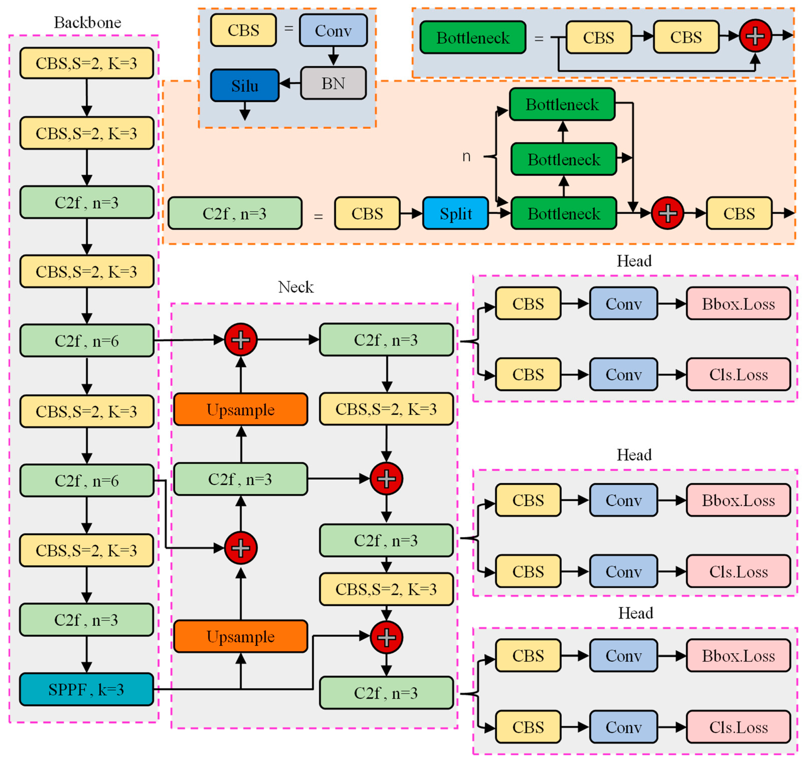
2.4. Bolt Detachment Defect Detection Algorithm

2.4.1. Target Detection Algorithm

In the realm of computer vision, the primary task of target detection algorithms is to detect the position and category of target objects in an image. According to the detection process, they can be categorized into one-stage and two-stage types [54]. The one-stage detection algorithm is a single regression problem and is mainly employed in real-time detection tasks. Typical algorithms include SSD and the YOLO series. The two-stage detection algorithm is a process of first proposing candidates and then performing regression, and is mainly used in high-precision detection tasks. Representative algorithms comprise Faster R-CNN, Mask R-CNN, and others.

To construct a real-time bolt detachment defect detection model with superior performance, this paper selects nine models such as the YOLO series for comparative analysis. Taking the YOLOv8 network as an example, its network structure is depicted in Figure 4.

The YOLOv8 model primarily consists of three parts: the backbone network (Backbone), the feature fusion network (Neck), and the detection head (Head) [55]. The Backbone uses a series of convolutions to perform multi-scale feature extraction on the input image. The C2f module integrates residual connections, making the network lighter, with more abundant gradient flow and stronger feature extraction capability. The neck is a feature pyramid network structure (FPN) [56] and acts as a bridge connecting the backbone and head. It further processes the multi-scale feature maps extracted by the backbone and uses upsampling and downsampling to achieve the fusion of low-level detailed features and high-level semantic features. The path aggregation network (PAN) [57] is utilized to achieve a cross-layer feature fusion to obtain multi-scale, comprehensive, and rich feature maps. The head is responsible for outputting the target detection results of three different scale images, all of which are composed of two parts: position and category. The position detection results are generated through a series of convolutional layers and deconvolutional layers, and the category detection results are generated by global average pooling of the feature maps. Different application scenarios can choose networks of different depths, such as Yolov8n, Yolov8s, Yolov8m, Yolov8l, and Yolov8x.

The loss function of the target detection model is composed of three parts: localization loss L_loc, confidence loss L_conf, and classification loss L_cls. The L_loc reflects the difference between the predicted box and the ground truth. The L_conf reflects the error of whether there is a target in the detection box. The L_cls reflects the difference between the predicted category and the real category, as shown in Equation (15) [54].

$$L_{all}={\lambda }_{loc}{L}_{loc}+{\lambda }_{conf}{L}_{conf}+{\lambda }_{cls}{L}_{cls}$$

(15)

where λ_loc, λ_conf, and λ_cls, respectively, represent the importance coefficients of each loss part.

The evaluation index of the target detection model can measure the performance of the model. This paper selects precision (p), recall (r), F₁ score, and mean average precision (mAP) as the model performance evaluation indexes. p and r reflect the precision and recall rate of the model and are single indexes for evaluating model performance. The F₁ score and mAP are comprehensive evaluation indexes of model performance that balance the relationship between p and r, as shown in Equation (16) [58].

$$p={\displaystyle \frac{TP}{TP+FP}}, r={\displaystyle \frac{TP}{TP+FN}}, F_1={\displaystyle \frac{2pr}{p+r}}, IoU={\displaystyle \frac{GT\cap PB}{GT\cup PB}}, mAP={\displaystyle \frac{1}{n}}{\displaystyle \sum _{i=1}^n{\displaystyle {\int }_0^{1}p(r)dr}}$$

(16)

where TP is the number of detection boxes that correctly predict positive samples, TN is the number of detection boxes that correctly predict negative samples, FP is the number of negative samples that are wrongly predicted as positive samples, FN is the number of positive samples that are wrongly predicted as negative samples. IoU is the intersection over union, GT is the ground truth, PB is the predicted box. n is the number of target detection categories, p(r) is the relationship curve function between p and r, and mAP is related to the threshold value taken by IoU. mAP_0.5 is the result calculated when IoU = 0.5.

2.4.2. Transfer Learning

After undergoing deep augmentation, the dataset has been expanded to a certain degree. However, directly applying it to train a target detection model from scratch would encounter issues such as poor robustness, poor generalization, and the high consumption of time and computational power. Transfer learning can effectively address this problem. Transfer learning [59] is a method in machine learning that can transfer the experience learned in the learning task of the source domain to the learning task of the target domain, thereby accelerating the learning of the target domain task. It can be used to resolve the contradictions between big data and few annotations, big data and weak computing capabilities, as well as universal models and personalized needs.

The stronger the correlation between the source domain and the target domain, the more excellent the learning effect after transfer. Here, the commonly used large-scale dataset COCO (Common Objects in Context) is selected as the source domain, which contains a total of 200,000 images in 80 categories. The randomly augmented bolt image dataset is taken as the target domain. In a convolutional neural network, the features extracted by each layer of convolution are different. Shallow convolution extracts rough geometric features and has a strong ability to be transferred to the target domain. In contrast, deep convolution extracts complex abstract features and has a weak ability to be transferred to the target domain. Transfer the relevant parameters obtained by training the target detection model on the COCO dataset to the target domain, and then fine-tune the network for the bolt target detection task to train a new bolt target detection classifier. The target detection model based on transfer learning is shown in Figure 5.

3. Experiments and Results

3.1. Preparation of Image Dataset

Consumer-grade cameras are employed to collect the images of bolt detachment defect. During the shooting process, the shooting angle, distance, and lighting conditions are varied to obtain as diverse images as possible. A total of 1000 bolt images are collected, as depicted in Figure 6. A small sample bolt image dataset is constructed for training the DCGAN network, thereby achieving the deep augmentation and expansion of the dataset.

3.2. Augmentation of Image Dataset

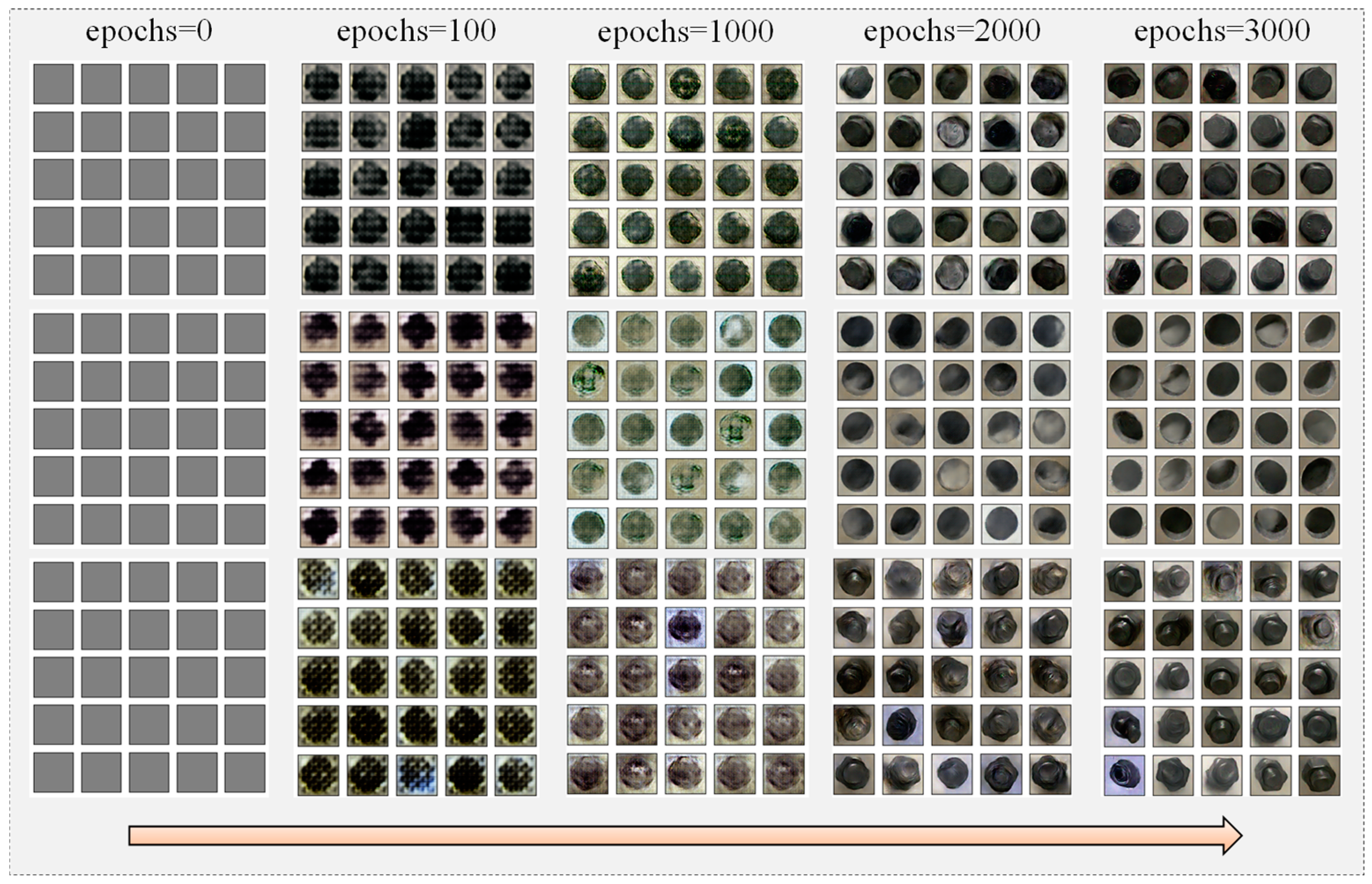
3.2.1. Training of DCGAN

The constructed DCGAN model is presented in

Table 1. Detailed parameters of the DCGAN model.

The Type of Network	Network Layer	Network Composition	Kernel Size	Stride	N_Out
Generator	G1	DeConv2d + BN + ReLU	4	1	512
	G2	DeConv2d + BN + ReLU	3	2	256
	G3	DeConv2d + BN + ReLU	3	3	128
	G4	DeConv2d + BN + ReLU	4	4	64
	G5	DeConv2d + BN + Tanh	6	4	64
Discriminator	D1	Conv2d + IN + LeakyReLU	6	4	64
	D2	Conv2d + IN + LeakyReLU	4	4	64
	D3	Conv2d + IN + LeakyReLU	3	3	128
	D4	Conv2d + IN + LeakyReLU	3	2	256
	D5	Conv2d	4	1	512

. In Table 1, G₁ to G₅ represent each layer of the generative network, D₁ to D₅ represent each layer of the discriminant network, Conv2d denotes a two-dimensional convolutional layer, DeConv2d represents a two-dimensional deconvolutional layer, instance normalization (IN), and batch normalization (BN) are regularization layers. ReLU, LeakyReLU, and Tanh are activation function layers, and N_out is the number of output convolution kernels.

The relevant hyperparameters of the model are set as follows: the learning rate, batch size, and epochs are 0.0002, 32, and 3000, respectively. The generated image sizes comprise three types: 32 × 32, 64 × 64, and 96 × 96. The training process is conducted on a desktop computer (CPU: Intel Core i5-13600KF (Intel Corporation, Santa Clara, CA, USA), 3.5 GHz, RAM 32G (Kingston Technology, Fountain Valley, CA, USA); GPU: RTX4060Ti (NVIDIA Corporation, Santa Clara, CA, USA) and 16 G).

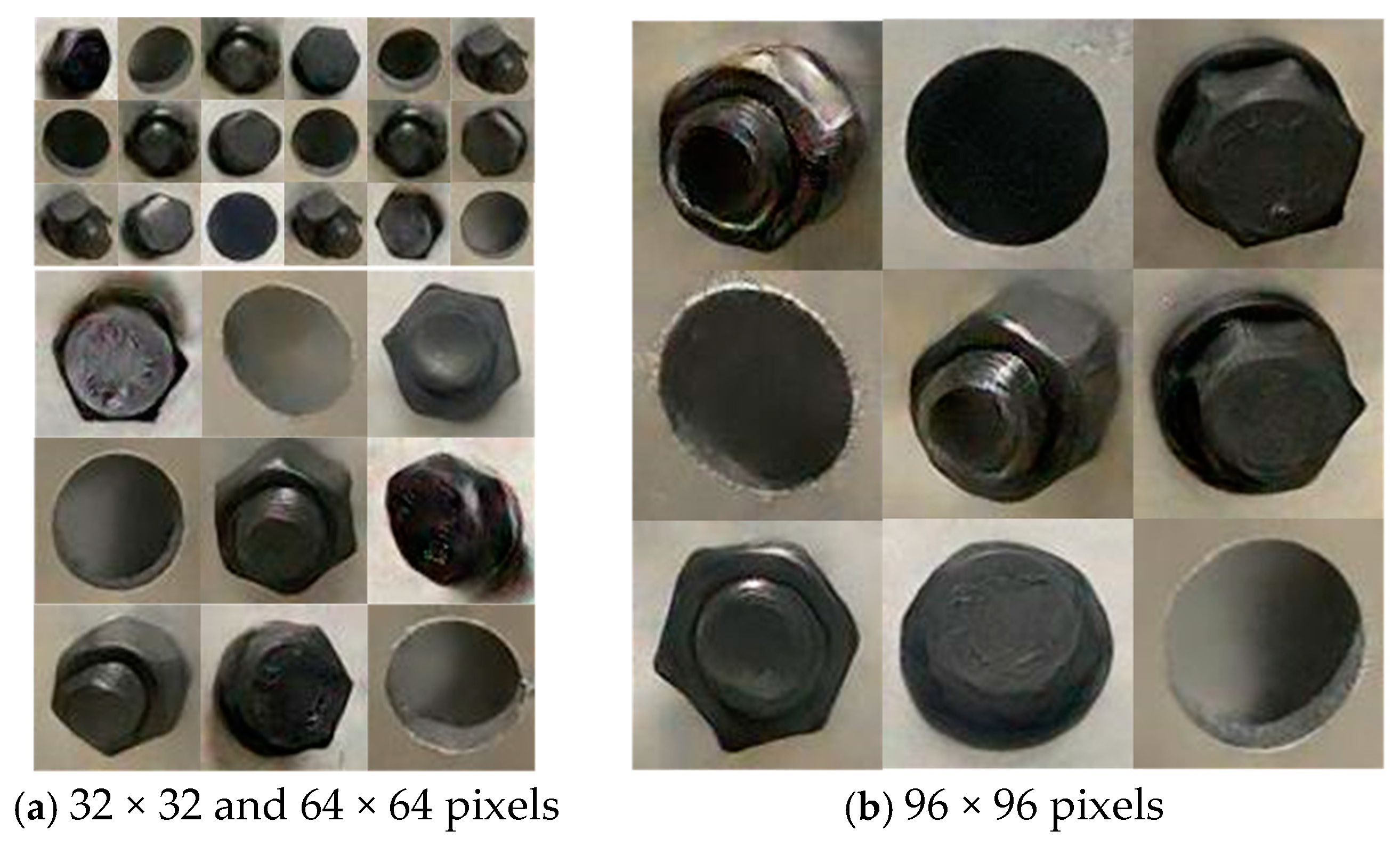
3.2.2. Image-Generation Results

The iterative training process of the model is shown in Figure 7. The generative network gradually learns the feature distribution of real images until it generates realistic pseudo-images. When epochs is 0, the model has not commenced learning yet, and the generated image is the input random noise. When epochs is 100, the model learns the low-level features such as edges and contours in real images. When epochs is 1000, the edge and contour features of the generated image are further learned, yet lack detailed features. When epochs is 2000, the model learns more detailed features in real images, but the image clarity is insufficient. When epochs is 3000, the generated image has abundant detailed features and is highly similar to the real image, making it impossible to distinguish authenticity. It can be utilized for the deep augmentation and expansion of the bolt image dataset.

The trained DCGAN network is used to generate bolt images of different sizes, as shown in Figure 8. The generated images are mixed with real images as dataset 1 for the subsequent training of the low-light enhancement network Zero-DCE++. The image annotation software LabelImg (version 1.8.6) is employed to annotate dataset 1 to obtain dataset 2 for the subsequent training of the target detection model.

3.2.3. Evaluation of Image Generation Quality

In addition to subjectively evaluating the quality of generated images, objective indicators such as MSE, PSNR, and SSIM should also be calculated to quantitatively assess the quality of generated images. The statistical results of the calculations are shown in

Table 2. Calculation results of the evaluation indicators for generated images.

Generate Images	Number of Images	Image Pixels	MSE (↓)	PSNR (↑)	SSIM (↑)
Bolt cap	200	32 × 32	24.18	15.16	0.48
	200	64 × 64	29.28	14.27	0.34
	200	96 × 96	23.07	15.32	0.39
Nut	200	32 × 32	12.13	17.45	0.49
	200	64 × 64	11.20	18.02	0.38
	200	96 × 96	9.11	18.81	0.49
Detachment	200	32 × 32	18.58	16.47	0.60
	200	64 × 64	16.14	16.99	0.58
	200	96 × 96	16.96	16.79	0.59

Note: In Table 2, ‘↓’ denotes that lower values indicate superior image quality, whereas ‘↑’ signifies higher values are preferable.

. It can be seen from Table 2 that, from the perspective of local similarity evaluation indicators (MSE and PSNR), the generated nut surface image is optimal. From the perspective of overall similarity evaluation indicators (SSIMs), the generated detachment image is the best, and the generated nut surface and bolt cap surface images are second in turn.

3.3. Training of Zero-DCE++

Zero-DCE++ is an unsupervised learning approach that does not depend on a large number of paired image datasets. To enhance the model’s ability to adjust the wide dynamic range, a series of images including low-light and overexposed ones are utilized as the training set. The image size of the dataset is uniformly adjusted to 512 × 512 × 3. The learning rate, batch size, and epochs of the model are set to 0.0001, 16, and 200, respectively. The ADAM optimizer is employed to optimize the model training process. The weight coefficients of the loss function are sequentially assigned as 1, 1, 0.5, and 20. The training equipment is the same as that for training DCGAN.

After the training of Zero-DCE++ is completed, the collected low-light images are input into Zero-DCE++, and the enhanced images obtained are shown in Figure 9. The mean brightness of the image is calculated according to Equation (17).

$$\mathrm{Mb}={\displaystyle \frac{1}{N}}{\displaystyle \frac{1}{M}}{\displaystyle \sum _i^N{\displaystyle \sum _j^M(0.299R_{i,j}+0.587G_{i,j}+0.114B_{i,j})}}$$

(17)

where Mb represents the mean brightness of the image, N × M represents the pixel size of the image, R_i,j, G_i,j, and B_i,j, respectively, denote the pixel values of each point in the red, green, and blue channels of the image.

As can be seen from Figure 9, for an ultra-low-light image with a mean brightness of 13.0817, the mean brightness of the enhanced image can reach 77.8556, with an increase of 64.7739. For a low-light image with a mean brightness of 37.0511, the mean brightness of the enhanced image can reach 117.1452, with an increase of 80.0941. This indicates that both ultra-low-light images and low-light images can be enhanced to different extents, and the enhancement degree of ultra-low-light images is weaker than that of low-light images. Therefore, by increasing the initial mean brightness of the captured image as much as possible, a better light enhancement effect can be achieved.

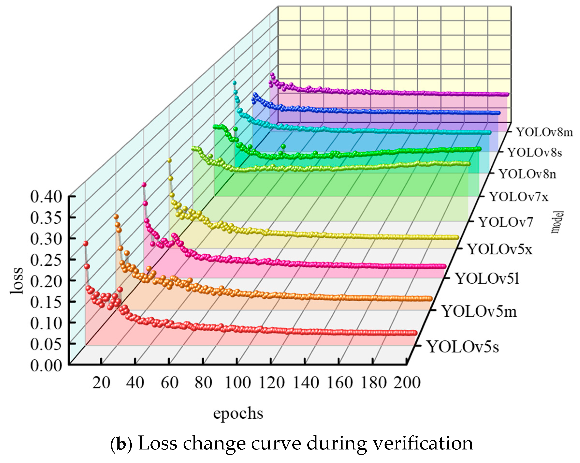
3.4. Training of Target Detection Model

Transfer the model parameters pre-trained in the COCO dataset to accelerate the training process of the target detection model herein. The relevant hyperparameters of the model are configured as follows: the learning rate, batch size, and epochs are 0.0001, 16, and 200, respectively. The training equipment is identical to that used for training DCGAN.

In this paper, nine models including YOLOv5, YOLOv7, and YOLOv8 are trained, respectively, to obtain the model with optimal performance. During the training process, the changing trends of the loss functions of different models on the training set and validation set are depicted in Figure 10.

The results indicate that each model reaches convergence after approximately 140 iterations in the training set and around 120 iterations in the validation set. By comparing the performance evaluation indicators to obtain the optimal model, the calculation results are shown in

Table 3. Comparison of model performance evaluation indicators.

Model	p (%)	r (%)	F1 (%)	mAP_0.5:0.95	Param (M)	Weight_Size (MB)	FPS (GPU)
YOLOv5s	96.48	97.69	97.08	84.69	7.0	14.5	476
YOLOv5m	96.30	97.70	96.99	83.92	20.9	42.3	371
YOLOv5l	96.85	97.67	97.26	86.39	46.2	92.9	244
YOLOv5x	97.16	97.72	97.44	86.40	86.2	173.2	154
YOLOv7	94.09	93.84	93.69	81.66	37.2	74.9	205
YOLOv7x	93.69	95.97	94.82	79.98	70.9	142.2	147
YOLOv8n	98.98	99.05	99.01	93.97	3.1	6.3	424
YOLOv8s	99.16	99.19	99.17	94.88	11.1	22.5	449
YOLOv8m	99.08	99.18	99.13	95.08	25.9	52.1	307

Note: In Table 3, the optimal evaluation metrics are marked in red bold font for emphasis.

. As the amount of model parameters increases, the inference speed decreases, and there is no significant difference in F₁. However, the mAP_0.5:0.95 of the YOLOv8 series models is notably higher than that of other models. To comprehensively balance the model accuracy and inference speed, YOLOv8n is selected for subsequent bolt detection.

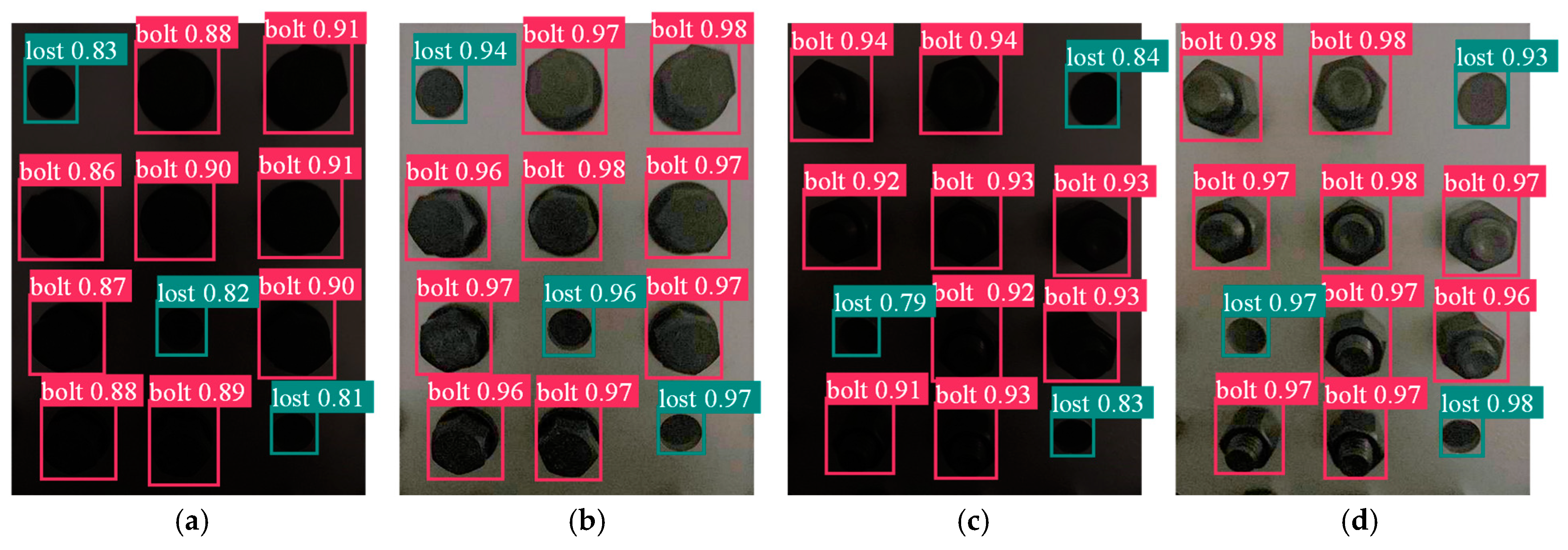
3.5. Bolt Detachment Defect Detection Results

The captured bolt images to be detected are classified according to the mean brightness. For images with a mean brightness lower than 75, light enhancement processing is performed first, followed by bolt detachment defect detection. The limit value of 75 is determined by the mean brightness after the ultra-low-light image is enhanced as described in Section 3.3. The detection results before and after low-light image enhancement are shown in Figure 11. As can be seen from Figure 11a,c, before the low-light image is enhanced, the average detection accuracy of bolt detachment is 82%. As can be seen from Figure 11b,d, after the low-light image is enhanced, the average detection accuracy of bolt detachment is 95.8%. Therefore, after light enhancement processing, both the accuracy and robustness of the bolt detachment detection model are improved.

3.6. Validation

To validate the generalization performance of the bolt detachment detection model, the spliced plate with a complex background in an engineering example is taken as the research object, and the bolt images under different shooting conditions are analyzed. The schematic of image acquisition is presented in Figure 12. The selected segment contains a total of 24 high-strength bolts, which are sequentially numbered from 1 to 24. Among them, bolts numbered 4, 7, 10, 18, 19, and 23 exhibit fractures and detachments.

The shooting angle θ is defined as the angle between the camera line of sight and the normal line of the spliced plate. The shooting distance d represents the horizontal distance between the camera and the spliced plate. The lighting environment is measured by the Mb of the image. The Mb (from 10 to 50), distance d (from 1.0 m to 2 m), and angle (from 0° to 40°) are varied, and a total of 12 working conditions are set as shown in

Table 4. Bolt image acquisition working conditions.

Working Conditions	Mb (10–50)	d (1.0–2 m)	$\mathit{\theta }$ (0°–40°)
I1–I4	10–20, 20–30, 30–40, 40–50	1.0 m	0°
I5–I8	20–30	1.0 m, 1.3 m, 1.6 m, 2.0 m	0°
I9–I12	20–30	1.0 m	10°, 20°, 30°, 40°

.

The bolt images collected under the working conditions I₁ to I₁₂ are shown in Figure 13a,c,e. After enhancement processing, they are presented in Figure 13b,d,f. The images taken under working conditions I₁ to I₁₂ are sequentially input into the Zero-DCE++ and the YOLOv8n, and the detection results are shown in

Table 5. Detection results under working conditions I1 to I12.

Conditions	Without Zero-dce++							With Zero-dce++
	4	7	10	18	19	23	FMR	4	7	10	18	19	23	FMR
I1	0.45	0.85	0.60	0.91	0.93	0.86	45.83%	0.93	0.95	0.91	0.95	0.94	0.95	0.00%
I2	0.76	0.91	0.65	0.91	0.91	0.89	33.33%	0.96	0.96	0.94	0.95	0.95	0.95	0.00%
I3	0.84	0.91	0.61	0.91	0.91	0.89	25.00%	0.96	0.95	0.93	0.94	0.96	0.95	0.00%
I4	0.88	0.91	0.63	0.91	0.91	0.90	20.83%	0.96	0.96	0.92	0.94	0.95	0.95	0.00%
I5	0.84	0.90	0.64	0.82	0.84	0.83	29.17%	0.95	0.94	0.93	0.95	0.96	0.94	0.00%
I6	0.76	0.85	/	0.85	0.87	0.83	33.33%	0.89	0.94	0.92	0.91	0.95	0.94	0.00%
I7	0.6	0.91	0.66	0.78	0.85	0.76	33.33%	0.9	0.96	0.95	0.88	0.92	0.80	4.17%
I8	/	0.89	0.62	0.61	0.79	0.76	50.00%	0.83	0.95	0.94	0.83	0.88	0.87	8.33%
I9	0.86	0.87	0.64	0.89	0.89	0.87	30.77%	0.92	0.96	0.95	0.95	0.95	0.89	0.00%
I10	0.6	0.85	/	0.91	0.89	0.89	19.23%	0.91	0.95	0.94	0.95	0.96	0.93	3.85%
I11	0.84	0.83	0.46	0.55	0.75	0.72	23.08%	0.94	0.93	0.93	0.93	0.93	0.93	3.85%
I12	0.46	0.53	0.41	/	0.73	0.53	30.77%	0.91	0.66	0.91	0.89	0.93	0.92	7.69%
global FMR	31.08%							2.36%

Note: In Table 5, FMR denotes the ratio of the sum of the number of detected category errors and the number not detected to the total number of targets. A larger value of this metric indicates a greater error.

.

As indicated in Table 5, when the image is not enhanced by Zero-DCE++, the bolt detachment detection accuracy is relatively low, and the false detection and missed detection rates are high. The global FMR can reach 31.08%. In working condition I₈, the maximum value of FMR appears as 50%. After the image is enhanced by Zero-DCE++, the bolt detachment detection accuracy shows a significant improvement, and the false detection and missed detection rates are significantly reduced. The global FMR is only 2.36%. Similarly, in working condition I₈, the maximum value of FMR is 8.33%. In working conditions I₇, I₁₀, I₁₁, and I₁₂, the FMRs are 4.17%, 3.85%, 3.85%, and 7.69%, respectively, suggesting that changing the shooting distance and angle can affect the detection performance of the model.

To explore the impact of different imaging conditions on the model’s detection performance, the average bolt detachment detection accuracy under working conditions I₁ to I₁₂ is compared and analyzed, as shown in Figure 14, thereby determining the optimal application conditions of the model.

As shown in Figure 14a, compared with the bolt images in low-light environments, after being enhanced by Zero-DCE++, the mean value of bolt detachment detection accuracy is improved to different extents, indicating that the Zero-DCE++ light enhancement network has excellent performance. Furthermore, as can be seen from Figure 14b, in working conditions I₁ to I₄, the Mb of the image increases in sequence. For images with lower Mb, the mean value of bolt detachment detection accuracy is increased to a greater degree after being enhanced by Zero-DCE++, but the mean value of accuracy after enhancement tends to stabilize.

According to Figure 14c, in working conditions I₅ to I₈, the image shooting distance increases from 1.0 m to 2.0 m. As the shooting distance increases, the mean value of bolt detachment detection accuracy after being enhanced by Zero-DCE++ shows a gradual downward trend. There is one and two false detections and missed detections in I₇ and I_8, respectively. This is because the increase in shooting distance leads to a rapid decrease in the resolution of the target area. At the same time, the complex background also exacerbates the detection difficulty, as evidenced in Figure 15. Therefore, controlling the shooting distance within 1.6 m as much as possible can improve the reliability of the model detection results. Moreover, as depicted in Figure 14d, in working conditions I₉ to I₁₂, the image shooting angle increases from 10° to 40°. As the shooting angle increases, the mean value of bolt detachment detection accuracy after being enhanced by Zero-DCE++ also shows a downward trend. There are one, one, and two false detections and missed detections in I₁₀, I₁₁, and I_12, respectively. This is because the increase in shooting angle leads to occlusion and background interference in the target area, as demonstrated in Figure 15. Consequently, controlling the shooting angle within 20° as much as possible can improve the reliability of the model detection results.

4. Conclusions

This study presents an automated detection method for bolt detachment defect in the low-light scenarios of wind turbines based on computer vision. The proposed approach combines generative image augmentation and expansion, low-light image enhancement, and a lightweight target detection model. Based on the above research, the following conclusions can be drawn:

(1)

The deep convolutional generative adversarial network (DCGAN) is demonstrated as an effective approach to augmenting image datasets by generating realistic bolt images, thereby enhancing both the quantity and quality of training data while diversifying feature distributions. This methodology provides a viable solution for few-shot learning scenarios, where limited annotated data are available.

(2)

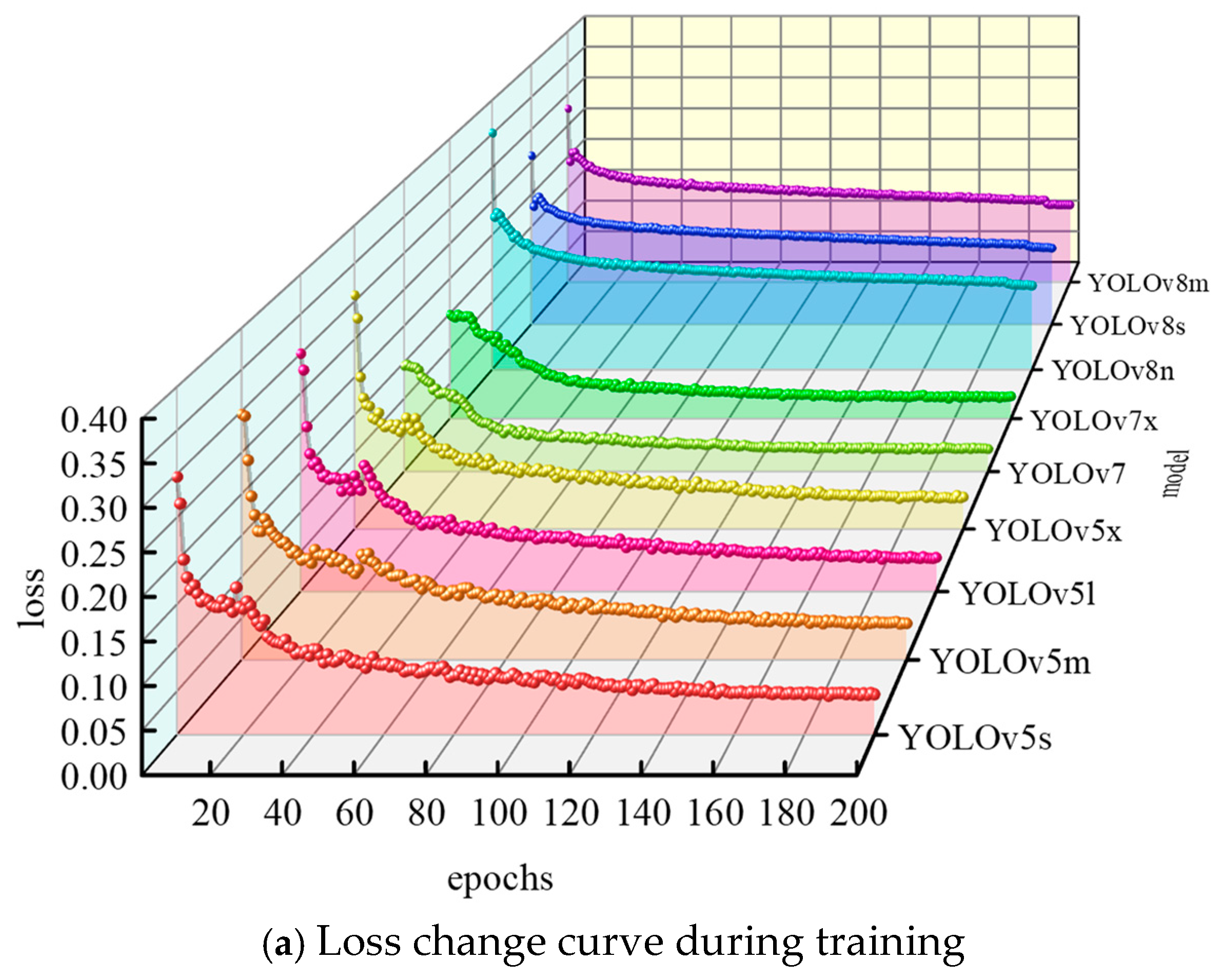
To optimize the detection performance, nine model variants—including YOLOv5, YOLOv7, and YOLOv8—are rigorously evaluated. After comprehensively balancing detection accuracy and computational efficiency, the YOLOv8n model is selected for bolt detachment defect detection. The model achieves a detection speed of 424 frames per second (FPSs) and a mean average precision (mAP@0.5:0.95) of 93.97%, enabling the high-precision real-time online monitoring of bolt defects in wind turbines.

(3)

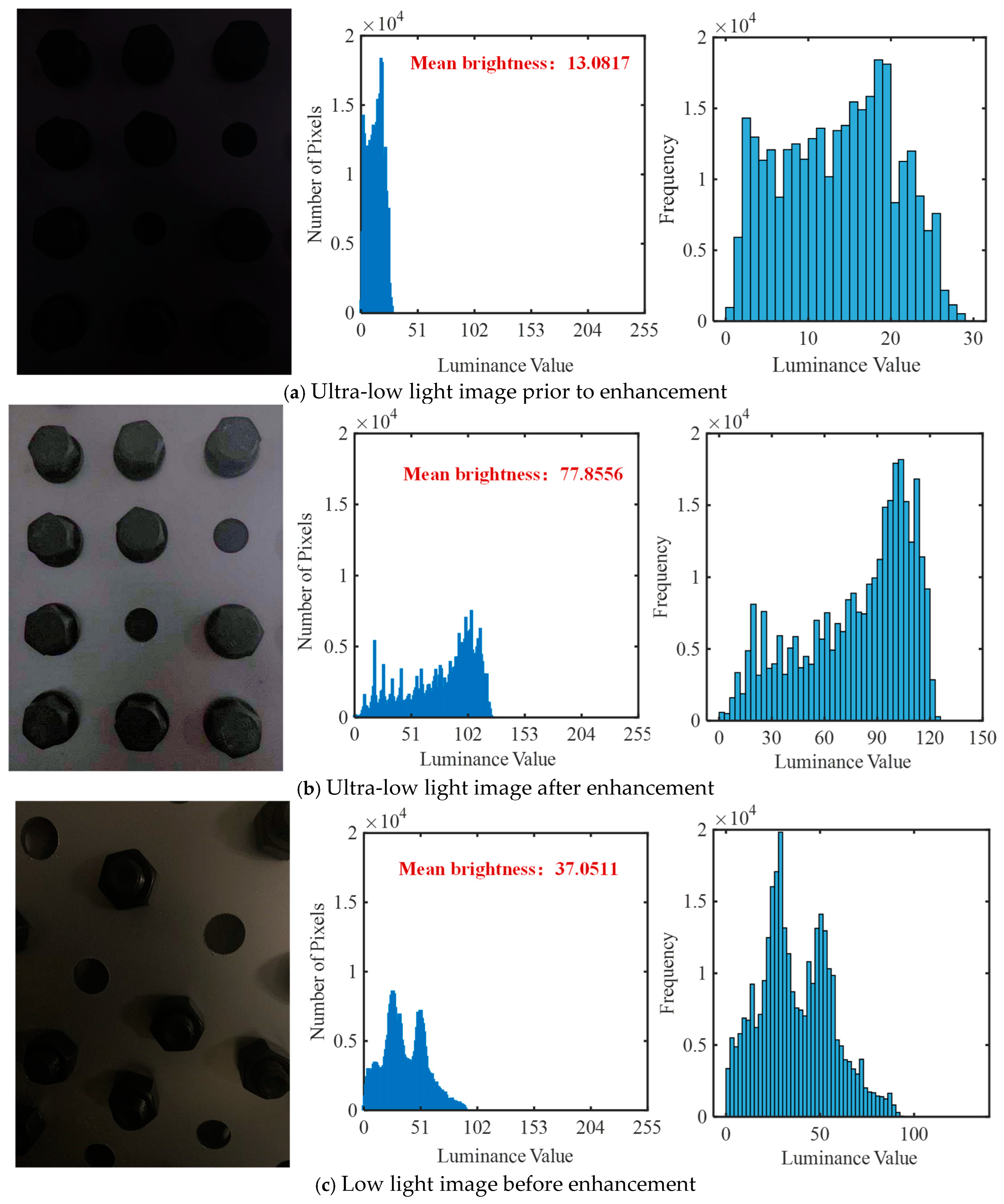
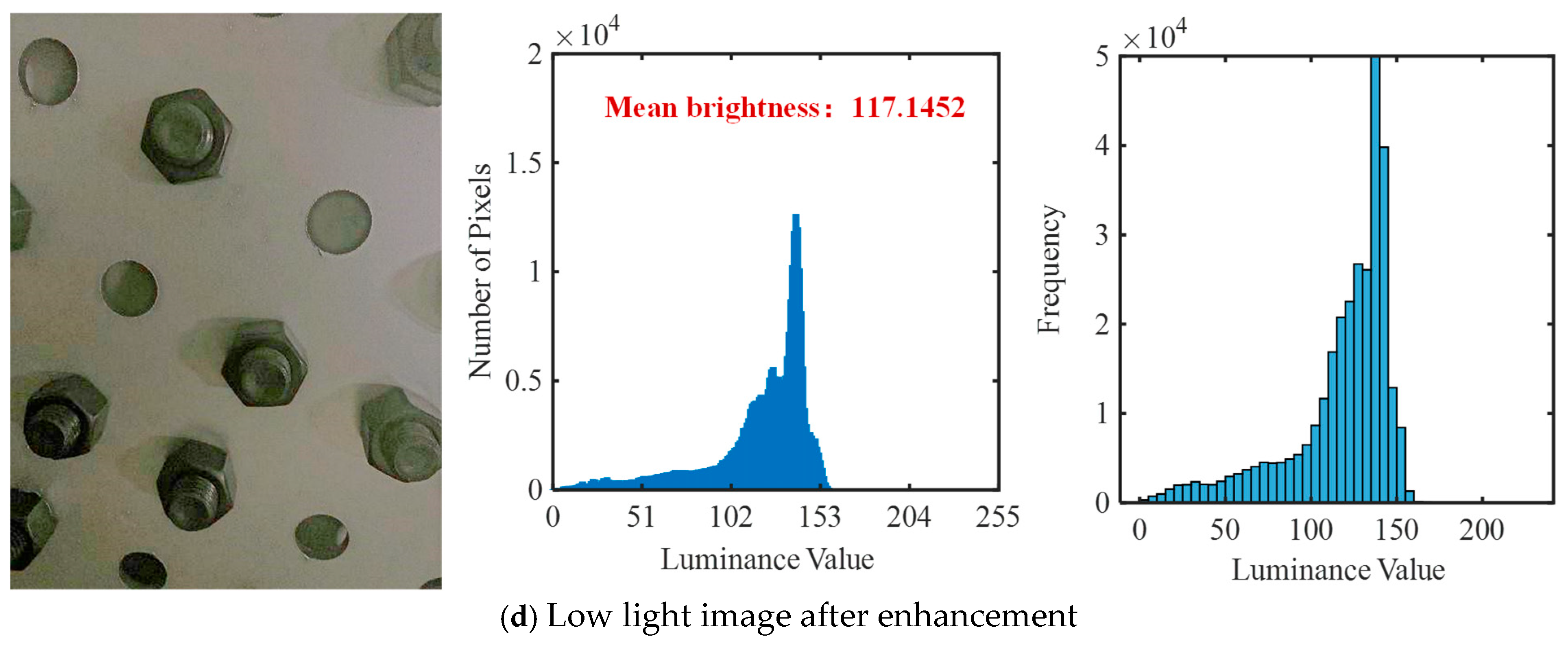
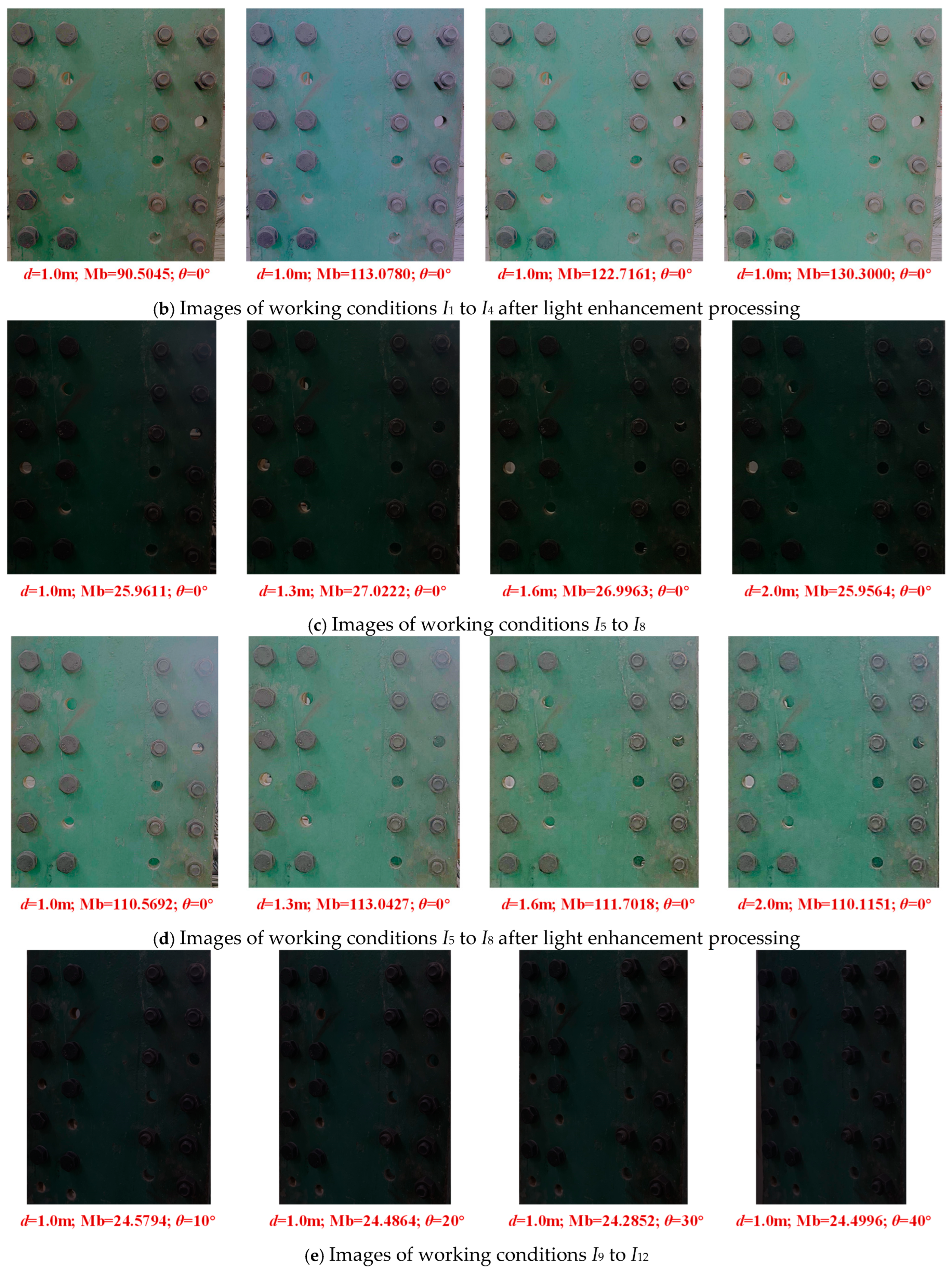
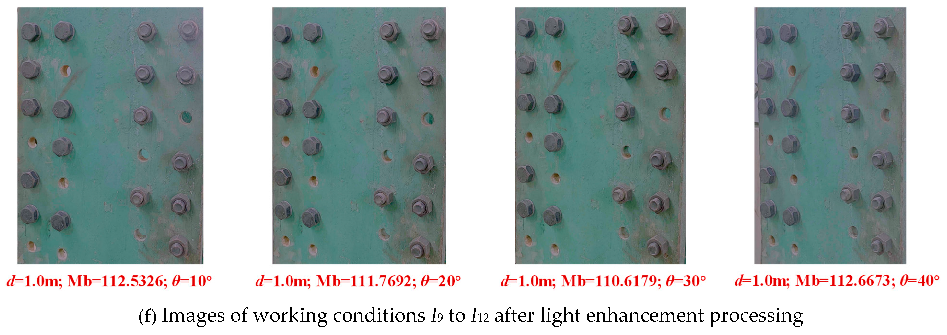
After bolt images under different imaging conditions are enhanced by the Zero-DCE++ algorithm, the Mb of bolt images is significantly increased. Moreover, after image enhancement, the bolt detachment detection error rate is reduced from 31.08% to 2.36%, and the bolt detachment detection accuracy is improved. However, changes in shooting distance and angle can affect the model’s detection performance. Controlling the shooting distance within 1.6 m and the shooting angle within 20° can greatly enhance the reliability of the model’s detection results. At this point, zero false detection and missed detection can be achieved.

(4)

For offshore applications, our method requires IP68-rated cameras mounted on inspection drones or robotic arms, paired with edge computing devices (e.g., NVIDIA Jetson AGX). Data transmission via 5G modules ensures real-time monitoring. Field deployment should prioritize anti-corrosion hardware and periodic model retraining using marine-environment datasets.

References

1. Cheng, L.; Yang, F.; Seidel, M.; Veljkovic, M. FE-assisted investigation for mechanical behaviour of connections in offshore wind turbine towers. Eng. Struct. 2023, 285, 116039. [Google Scholar] [CrossRef]
2. Tran, T.-T.; Lee, D. Understanding the behavior of l-type flange joint in wind turbine towers: Proposed mechanisms. Eng. Fail. Anal. 2022, 142, 106750. [Google Scholar] [CrossRef]
3. Mar, A.M.; José, M.A.; Felipe, P.Á.R.; Juan, J.D.C.D. Wind turbine tower collapse due to flange failure: FEM and DOE analyses. Eng. Fail. Anal. 2019, 104, 932–949. [Google Scholar]
4. Du, J.; Qiu, Y.; Wang, Z.; Li, J.; Wang, H.; Wang, Z.; Zhang, J. A Three-Stage Criterion to Reveal the Bolt Self-Loosening Mechanism Under Random Vibration by Strain Detection. Eng. Fail. Anal. 2022, 133, 105954. [Google Scholar] [CrossRef]
5. Ma, T.; Feng, Q.; Tan, Z.; Ou, J. Optical phase mode analysis method for pipeline bolt looseness identification using distributed optical fiber acoustic sensing. Struct. Health Monit. 2024, 23, 1547–1559. [Google Scholar] [CrossRef]
6. Chen, Y.; Wu, W.; Wu, J.; Wang, J.; Li, W. Experimental Evaluation of Wearable Piezo Ring for Bolted Connection Monitoring Using the Active Sensing Approach. IEEE Sens. J. 2023, 23, 4430–4437. [Google Scholar] [CrossRef]
7. Qin, X.; Peng, C.; Zhao, G.; Ju, Z.; Lv, S.; Jiang, M.; Sui, Q.; Jia, L. Full life-cycle monitoring and earlier warning for bolt joint loosening using modified vibro-acoustic modulation. Mech. Syst. Signal Process 2022, 162, 108054. [Google Scholar] [CrossRef]
8. Zhou, L.; Chen, S.-X.; Ni, Y.-Q.; Choy, A.W.-H. EMI-GCN: A hybrid model for real-time monitoring of multiple bolt looseness using electromechanical impedance and graph convolutional networks. Smart Mater. Struct. 2021, 30, 035032. [Google Scholar] [CrossRef]
9. Zhou, Y.; Wang, S.; Zhou, M.; Chen, H.; Yuan, C.; Kong, Q. Percussion-based bolt looseness identification using vibration-guided sound reconstruction. Struct. Control Health Monit. 2022, 29, e2876. [Google Scholar] [CrossRef]
10. Han, C.; Wang, S.; Madan, A.; Zhao, C.; Mohanty, L.; Fu, Y.; Shen, W.; Liang, R.; Huang, E.S.; Zheng, T.; et al. Intelligent detection of loose fasteners in railway tracks using distributed acoustic sensing and machine learning. Eng. Appl. Artif. Intell. 2024, 134, 108684. [Google Scholar] [CrossRef]
11. Wang, F.; Chen, Z.; Song, G. Monitoring of multi-bolt connection looseness using entropy-based active sensing and genetic algorithm-based least square support vector machine. Mech. Syst. Signal Process 2020, 136, 106507. [Google Scholar] [CrossRef]
12. Luo, J.; Zhao, J.; Sun, Y.; Liu, X.; Yan, Z. Bolt-loosening detection using vision technique based on a gray gradient enhancement method. Adv. Struct. Eng. 2023, 26, 668–678. [Google Scholar] [CrossRef]
13. Han, Q.; Wang, S.; Fang, Y.; Wang, L.; Du, X.; Li, H.; He, Q.; Feng, Q. A Rail Fastener Tightness Detection Approach Using Multi-source Visual Sensor. Sensors 2020, 20, 1367. [Google Scholar] [CrossRef] [PubMed]
14. Wang, C.; Wang, N.; Ho, S.-C.; Chen, X.; Song, G.; Ho, M. Design of a New Vision-Based Method for the Bolts Looseness Detection in Flange Connections. IEEE Trans. Ind. Electron. 2020, 67, 1366–1375. [Google Scholar] [CrossRef]
15. Ta, Q.-B.; Kim, J.-T. Monitoring of Corroded and Loosened Bolts in Steel Structures via Deep Learning and Hough Transforms. Sensors 2020, 20, 6888. [Google Scholar] [CrossRef]
16. Wang, Q.; Zhang, H.; Lin, C.; Yang, Y. A New Bolts-Loosening Detection Method in High-Voltage Tower Based on Binocular Vision. In Proceedings of the 2023 29th International Conference on Mechatronics and Machine Vision in Practice (M2VIP), Queenstown, New Zealand, 21–24 November 2023; pp. 90–99. [Google Scholar]
17. Huynh, T.-C. Vision-based Autonomous Bolt-Looseness Detection Method for Splice Connections: Design, Lab-Scale Evaluation, and Field Application. Autom. Constr. 2021, 124, 103591. [Google Scholar] [CrossRef]
18. Yuan, C.; Chen, W.; Hao, H.; Kong, Q. Near real-time bolt-loosening detection using mask and region-based convolutional neural network. Struct. Control Health Monit. 2021, 28. [Google Scholar] [CrossRef]
19. Wu, Y.; Qin, Y.; Qian, Y.; Guo, F. Automatic Detection of Arbitrarily Oriented Fastener Defect in High-Speed Railway. Autom. Constr. 2021, 131, 103913. [Google Scholar] [CrossRef]
20. Mushtaq, F.; Ramesh, K.; Deshmukh, S.; Ray, T.; Parimi, C.; Tandon, P.; Jha, P.K. Nuts&bolts: YOLO-v5 and image processing based component identification system. Eng. Appl. Artif. Intell. 2023, 118, 105665. [Google Scholar] [CrossRef]
21. Zhang, C.; Chen, X.; Liu, P.; He, B.; Li, W.; Song, T. Automated detection and segmentation of tunnel defects and objects using YOLOv8-CM. Tunn. Undergr. Space Technol. 2024, 150, 105857. [Google Scholar] [CrossRef]
22. Lu, Q.; Jing, Y.; Zhao, X. Bolt Loosening Detection Using Key-Point Detection Enhanced by Synthetic Datasets. Appl. Sci. 2023, 13, 2020. [Google Scholar] [CrossRef]
23. Bolton, T.; Bass, J.; Gaber, T.; Mansouri, T. Comparing Object Recognition Models and Studying Hyperparameter Selection for the Detection of Bolts. In NLDB, 2023; Lecture Notes in Computer Science; Springer: Cham, Switzerland, 2023; Volume 13913, pp. 186–200. [Google Scholar]
24. Yu, Y.; Liu, Y.; Chen, J.; Jiang, D.; Zhuang, Z.; Wu, X. Detection Method for Bolted Connection Looseness at Small Angles of Timber Structures based on Deep Learning. Sensors 2021, 21, 3106. [Google Scholar] [CrossRef] [PubMed]
25. Ian, J.G.; Jean, P.-A.; Mehdi, M.; Xu, B.; David, W.-F.; Sherjil, O.; Aaron, C.; Yoshua, B. Generative Adversarial Networks. arXiv 2014, arXiv:1406.2661. [Google Scholar]
26. Connor, S.; Taghi, M.K. A Survey on Image Data Augmentation for Deep Learning. J. Big Data 2019, 6, 60. [Google Scholar]
27. Zhou, Y.; Wang, B.; He, X.; Cui, S.; Shao, L. DR-GAN: Conditional Generative Adversarial Network for Fine-Grained Lesion Synthesis on Diabetic Retinopathy Images. IEEE J. Biomed. Health Inform. 2022, 26, 56–66. [Google Scholar] [CrossRef]
28. Zhang, W.; Zhang, P.; Yu, Y.; Li, X.; Biancardo, S.A.; Zhang, J. Missing Data Repairs for Traffic Flow With Self-Attention Generative Adversarial Imputation Net. IEEE Trans. Intell. Transp. Syst. 2022, 23, 7919–7930. [Google Scholar] [CrossRef]
29. Li, J.; Chen, Z.; Cheng, L.; Liu, X. Energy data generation with Wasserstein Deep Convolutional Generative Adversarial Networks. Energy 2022, 257, 124694. [Google Scholar] [CrossRef]
30. Lu, Y.; Chen, D.; Olaniyi, E.; Huang, Y. Generative Adversarial Networks (GANs) for Image Augmentation in Agriculture: A Systematic Review. Comput. Electron. Agric. 2022, 200, 107208. [Google Scholar] [CrossRef]
31. Pan, X.; Tavasoli, S.; Yang, T.Y. Autonomous 3D Vision-Based Bolt Loosening Assessment Using Micro Aerial Vehicles. Comput. Civ. Infrastruct. Eng. 2023, 38, 2443–2454. [Google Scholar] [CrossRef]
32. Du, F.; Wu, S.; Xu, C.; Yang, Z.; Su, Z. Electromechanical Impedance Temperature Compensation and Bolt Loosening Monitoring Based on Modified Unet and Multitask Learning. IEEE Sens. J. 2023, 23, 4556–4567. [Google Scholar] [CrossRef]
33. Luo, P.; Wang, B.; Wang, H.; Ma, F.; Ma, H.; Wang, L. An Ultrasmall Bolt Defect Detection Method for Transmission Line Inspection. IEEE Trans. Instrum. Meas. 2023, 72, 5006512. [Google Scholar] [CrossRef]
34. Li, C.; Guo, J.; Porikli, F.; Pang, Y. LightenNet: A Convolutional Neural Network for weakly illuminated image enhancement. Pattern Recognit. Lett. 2018, 104, 15–22. [Google Scholar] [CrossRef]
35. Zhang, Y.; Zhang, J.; Guo, X. Kindling the Darkness: A Practical Low-light Image Enhancer. In Proceedings of the 27th ACM International Conference on Multimedia (MM’19), Nice, France, 21–25 October 2019. [Google Scholar]
36. Zhang, Y.; Guo, X.; Ma, J.; Liu, W.; Zhang, J. Beyond Brightening Low-light Images. Int. J. Comput. Vis. 2021, 129, 1013–1037. [Google Scholar] [CrossRef]
37. Jiang, Y.; Gong, X.; Liu, D.; Cheng, Y.; Fang, C.; Shen, X.; Yang, J.; Zhou, P.; Wang, Z. EnlightenGAN: Deep Light Enhancement Without Paired Supervision. IEEE Trans. Image Process 2021, 30, 2340–2349. [Google Scholar] [CrossRef]
38. Ma, L.; Ma, T.; Liu, R.; Fan, X.; Luo, Z. Toward Fast, Flexible, and Robust Low-Light Image Enhancement. IEEE Conf. Comput. Vis. Pattern Recognit. 2022, 2022, 5627–5636. [Google Scholar]
39. Guo, C.; Li, C.; Guo, J.; Chen, C.L.; Hou, J.; Sam, K. Zero-Reference Deep Curve Estimation for Low-Light Image Enhancement. In Proceedings of the IEEE Computer Society Conference on Computer Vision and Pattern Recognition, Seattle, WA, USA, 13–19 June 2020; pp. 1777–1786. [Google Scholar]
40. Li, C.; Guo, C.; Chen, C.L. Learning to Enhance Low-Light Image via Zero-Reference Deep Curve Estimation. IEEE Trans. Pattern Anal. Mach. Intell. 2021, 44, 4225–4238. [Google Scholar] [CrossRef]
41. Gao, F.; Qian, C.; Xu, L.; Liu, J.; Zhang, H. An experimental study on the identification of the root bolts’ state of wind turbine blades using blade sensors. Wind. Energy 2024, 27, 363–381. [Google Scholar] [CrossRef]
42. Sethi, M.R.; Subba, A.B.; Faisal, M.; Sahoo, S.; Raju, D.K. Fault diagnosis of wind turbine blades with continuous wavelet transform based deep learning model using vibration signal. Eng. Appl. Artif. Intell. 2024, 138, 109372. [Google Scholar] [CrossRef]
43. Guan, Y.; Meng, Z.; Gu, F.; Cao, Y.; Li, D.; Miao, X.; Ball, A.D. Fault diagnosis of wind turbine structures with a triaxial vibration dual-branch feature fusion network. Reliab. Eng. Syst. Saf. 2025, 256, 110746. [Google Scholar] [CrossRef]
44. Liu, P.; Wang, X.; Wang, Y.; Zhu, J.; Ji, X. Research on percussion-based bolt looseness monitoring under noise interference and insufficient samples. Mech. Syst. Signal Process 2024, 208, 111013. [Google Scholar] [CrossRef]
45. Wang, X.; Yue, Q.; Liu, X. Bolted lap joint loosening monitoring and damage identification based on acoustic emission and machine learning. Mech. Syst. Signal Process 2024, 220, 111690. [Google Scholar] [CrossRef]
46. Fu, W.; Zhou, R.; Guo, Z. Automatic bolt tightness detection using acoustic emission and deep learning. Structures 2023, 55, 1774–1782. [Google Scholar] [CrossRef]
47. Li, D.; Nie, J.-H.; Wang, H.; Ren, W.-X. Loading condition monitoring of high-strength bolt connections based on physics-guided deep learning of acoustic emission data. Mech. Syst. Signal Process 2024, 206, 110908. [Google Scholar] [CrossRef]
48. Yang, X.; Gao, Y.; Fang, C.; Zheng, Y.; Wang, W. Deep learning-based bolt loosening detection for wind turbine towers. Struct. Control Health Monit. 2022, 29, e2943. [Google Scholar] [CrossRef]
49. Zhao, Y.; Zhang, Y.; Wang, J.; Yue, Q.; Chen, H. Comparison of non-destructive testing methods of bolted joint status in steel structures. Measurement 2025, 242, 116318. [Google Scholar] [CrossRef]
50. Alec, R.; Luke, M.; Soumith, C. Unsupervised Representation Learning with Deep Convolutional Generative Adversarial Networks. arXiv 2015, arXiv:1511.06434. [Google Scholar]
51. Ruder, S. An overview of gradient descent optimization algorithms. arXiv 2016, arXiv:1609.04747. [Google Scholar]
52. Sara, U.; Akter, M.; Uddin, M.S. Image Quality Assessment Through FSIM, SSIM, MSE and PSNR—A Comparative Study. J. Comput. Commun. 2019, 7, 8–18. [Google Scholar] [CrossRef]
53. Zhou, W.; Conrad, A.B.; Rahim, H.S.; Eero, S. Image quality assessment: From error visibility to structural similarity. IEEE Trans. Image Process 2004, 13, 600–612. [Google Scholar] [CrossRef]
54. Zou, Z.; Chen, K.; Shi, Z.; Guo, Y.; Ye, J. Object Detection in 20 Years: A Survey. Proc. IEEE 2019, 111, 257–276. [Google Scholar] [CrossRef]
55. Regin, V.; Sambath, M. YOLOv8: A Novel Object Detection Algorithm with Enhanced Performance and Robustness. In Proceedings of the 2024 International Conference on Advances in Data Engineering and Intelligent Computing Systems (ADICS), Chennai, India, 18–19 April 2024; pp. 1–6. [Google Scholar]
56. Lin, T.-Y.; Dollár, P.; Girshick, R.; He, K.; Hariharan, B.; Belongie, S. Feature Pyramid Networks for Object Detection. In Proceedings of the 2017 IEEE Conference on Computer Vision and Pattern Recognition (CVPR), Honolulu, HI, USA, 21–26 July 2017. [Google Scholar]
57. Liu, S.; Qi, L.; Qin, H.; Shi, J.; Jia, J. Path Aggregation Network for Instance Segmentation. In Proceedings of the IEEE Computer Society Conference on Computer Vision and Pattern Recognition, Salt Lake City, UT, USA, 18–23 June 2018; pp. 8759–8768. [Google Scholar]
58. Zhuang, L.; Qi, H.; Wang, T.; Zhang, Z. A Deep-Learning-Powered Near-Real-Time Detection of Railway Track Major Components: A Two-Stage Computer-Vision-Based Method. IEEE Internet Things J. 2022, 9, 18806–18816. [Google Scholar] [CrossRef]
59. Zhuang, F.; Qi, Z.; Duan, K.; Xi, D.; Zhu, Y.; Zhu, H.; Xiong, H.; He, Q. A Comprehensive Survey on Transfer Learning. Proc. IEEE 2021, 109, 43–76. [Google Scholar] [CrossRef]
Figure 1. Bolt detachment defect detection frame.
Energies 18 02197 g001
Figure 2. DCGAN structure diagram.
Energies 18 02197 g002
Figure 3. Zero-DCE++ network structure.
Energies 18 02197 g003
Figure 4. Yolov8 network structure.
Energies 18 02197 g004
Figure 5. Transfer learning-based object detection model.
Energies 18 02197 g005
Figure 6. An example of a bolt detachment image.
Energies 18 02197 g006
Figure 7. Iterative training process of the model.
Energies 18 02197 g007
Figure 8. Examples of generated images.
Energies 18 02197 g008
Figure 9. Results of image light enhancement.
Energies 18 02197 g009aEnergies 18 02197 g009b
Figure 10. Change curves of loss functions of various models.
Energies 18 02197 g010aEnergies 18 02197 g010b
Figure 11. Detection results of low-light bolt images before and after enhancement. (a) Low illumination on the nut surface. (b) Enhanced nut surface. (c) Low illumination on the bolt cap surface. (d) Enhanced bolt cap surface.
Energies 18 02197 g011
Figure 12. Schematic diagram of image acquisition.
Energies 18 02197 g012
Figure 13. Images of working conditions I1 to I12.
Energies 18 02197 g013aEnergies 18 02197 g013bEnergies 18 02197 g013c
Figure 14. Comparison of mean bolt detachment detection accuracy under working conditions I1 to I12.
Energies 18 02197 g014
Figure 15. Examples of typical bolt detachment image interference.
Energies 18 02197 g015