Energy Management Strategy for Fuel Cell Vehicles Based on Deep Transfer Reinforcement Learning

Abstract

Deep reinforcement learning has been widely applied in energy management strategies (EMS) for fuel cell vehicles because of its excellent performance in the face of complex environments. However, when driving conditions change, deep reinforcement learning-based EMS needs to be retrained to adapt to the new data distribution, which is a time-consuming process. To address this limitation and enhance the generalization ability of EMS, this paper proposes a deep transfer reinforcement learning framework. First, we designed a DDPG algorithm combined with prioritized experience replay (PER) as the research algorithm and trained a PER–DDPG-based EMS (defined as the source domain) using multiple driving cycles. Then, transfer learning was used when training the EMS (defined as the target domain) using a new driving cycle, i.e., the neural network parameters in the source domain model were reused to help initialize the target domain model. The simulation results show that the energy management strategy combined with transfer learning not only converges faster (improved by 59.09%), but also shows stronger adaptability when faced with new and more complex driving cycles, compared with not using transfer learning and having the model retrained.

1. Introduction

Traditional internal combustion engine vehicles rely on fossil fuels, posing serious challenges to environmental protection and energy security. Fuel cell vehicles, which use hydrogen as fuel and produce no greenhouse gas emissions, have emerged as a promising alternative to internal combustion engine vehicles [1,2]. Hydrogen energy holds great potential in the future new-energy landscape, and water electrolysis is one of the primary methods for producing hydrogen, offering both environmental friendliness and operational flexibility [3]. Currently, fuel cell vehicles are usually equipped with a traction battery as an auxiliary power source to provide instantaneous high-power output for the electric motor. However, the dual power source system is highly complex and requires effective coordination to maximize its advantages, making an efficient energy management strategy (EMS) particularly important [4,5,6]. Furthermore, the development of fuel cells is constrained by their operational lifespan. Numerous experiments have shown that frequent start–stop cycles and large power fluctuations readily accelerate degradation of the fuel cell’s internal structure. Therefore, in addition to minimizing energy losses, an effective EMS should also smooth the fuel cell’s power output to ensure stable operation [7].

There are three main types of existing EMS: rule-based, optimization-based, and learning-based [8,9]. Rule-based EMS rely on engineers’ experience and intuition, with a relatively simple design and low computation, but they are difficult to adapt to complex environments and are poorly optimized [10]. Optimization-based EMS seek the global optimal solution by constructing mathematical models, with typical methods including dynamic programming (DP). Although the optimization effect is significant, it is highly dependent on the model accuracy and needs to predict the working conditions, so it is usually used as a theoretical comparison benchmark [11]. Learning-based energy management strategies have demonstrated strong robustness in handling multi-objective complex tasks and are becoming a new solution by eliminating the reliance on predictions of future operational data [12,13].

Among these, deep reinforcement learning (DRL), through interaction with the environment, can optimize energy management strategies and make high-quality decisions, making it a current research hotspot [14]. DRL combines the advantages of deep learning and reinforcement learning, introducing deep neural networks (DNNs) on the basis of traditional reinforcement learning Q-learning, enabling reinforcement learning to handle high-dimensional state spaces [15]. The deep Q-network (DQN) is the earliest successfully applied DRL algorithm and has been widely used in the field of energy management. Lee et al. proposed a DQN-based EMS, which, compared to the equivalent consumption minimization strategy (ECMS), can achieve optimal control without relying on complex models. This research showcases the potential of the artificial intelligence technology in vehicle energy management, especially under complex driving conditions [16]. The DQN algorithm suffers from the problem of overestimated Q-values, and many studies have applied the improved double DQN algorithm to address this issue [17,18,19]. While the DQN solves the problem of traditional reinforcement learning being difficult to apply in high-dimensional spaces, it is still limited to discrete action spaces and struggles to meet the needs of continuous control problems. To address this, scholars have developed deep reinforcement learning algorithms based on the actor–critic architecture, with the most representative being the deep deterministic policy gradient (DDPG) [20]. In the DDPG, the actor network directly outputs a continuous action in each state, unlike the DQN which searches for the optimal action by traversing a discrete action space. The critic network, similar to the DQN, evaluates the actions generated by the actor network and outputs the corresponding Q-value for that action. Hu et al. proposed a DDPG-based EMS, employing a dual-architecture critic network and introducing a pre-training phase before the reinforcement learning process. Experimental results showed that the gap between this method and the benchmark DP strategy was reduced to 6.4% [21]. Besides the DDPG, the soft actor–critic (SAC) and twin delayed deep deterministic policy gradient (TD3) are also common DRL algorithms based on the actor–critic architecture. Wu et al. developed an SAC-based EMS for hybrid electric buses (HEBs), achieving a balance among multiple conflicting objectives and effectively optimizing energy distribution [22]. Liu et al. studied a battery-supercapacitor hybrid electric vehicle EMS based on the TD3 algorithm, with experimental results showing that the economic gap compared to DP-based EMS was reduced to 3% [23].

Although DRL has demonstrated outstanding performance in the EMS field, it still suffers from low training efficiency and limited generalization ability. To address these issues, the current research trend is to integrate DRL with other algorithms, such as combining DRL with rule-based or optimization-based EMS. Hu Yue et al. designed a DRL-based supplementary learning controller (SLC) and then combined it with a rule-based EMS to enhance the algorithm’s stability [24]. Wu et al. effectively reduced unreasonable exploration in the action space of DRL algorithms by introducing a rule-based mode control mechanism, with experimental results showing that the gap between this strategy and the DP-based strategy was narrowed to 2.55% [25]. In the development of EMS for fuel cell vehicles, the trend of integrating DRL algorithms with other strategies has become more pronounced. Li et al. developed an EMS for fuel cell buses structured in two levels: the upper-level framework integrates model predictive control (MPC) with reinforcement learning algorithms, while the lower-level framework employs an optimization-based strategy. Experimental results show that this hybrid EMS achieves a 3.59% improvement in energy savings compared to an EMS based on a single algorithm [26]. Zhou et al. designed an EMS for fuel cell trucks by combining artificial potential field (APF) functions with the DDPG algorithm; compared to an EMS based on the equivalent consumption minimization strategy (ECMS), this composite approach demonstrates strong synergy and reduces overall fuel costs [27].

In addition to the methods mentioned above, combining DRL with transfer learning (TL) offers a novel solution. Transfer learning is a machine learning approach whose core idea is to reuse the knowledge (e.g., saved parameters) acquired from a source task in a target task. This helps the target model initialize quickly, enabling it to reach satisfactory performance after a relatively short period of training [28,29]. Traditional DRL-based EMS are usually customized for a specific vehicle model or driving condition and thus require retraining whenever the environment changes. By integrating DRL and TL, one can fully capitalize on both technologies: DRL’s adaptive learning ability to handle complex and dynamic environments and TL’s capability to swiftly adapt to new scenarios. Researchers have already studied the application of TL in the EMS field. For example, Lian et al. used a Toyota Prius’s EMS as a pretrained model and transferred its knowledge to the EMS of three other hybrid vehicles with different structures, demonstrating that, compared to training from scratch, transfer learning can significantly reduce development time [30]. Lu et al. developed an EMS for fuel cell vehicles based on vehicle speed prediction, employing transfer learning to improve speed forecasting across operating conditions. Compared with schemes that do not use transfer learning, this strategy significantly reduces prediction errors [31].

To summarize, although the existing research on DRL-based EMS has already yielded numerous achievements, there remain several shortcomings:

• Most studies that apply TL focus on the improvement in convergence speed it brings, while overlooking the optimization of energy distribution performance.
• Research on TL is not sufficiently in-depth. Because of differences between the source task and the target task, TL may introduce certain negative effects. How to avoid these issues and use TL appropriately is still an open problem.

To address these issues, we designed an EMS that integrates DRL and TL for handling complex driving conditions. The main contributions of this study are as follows:

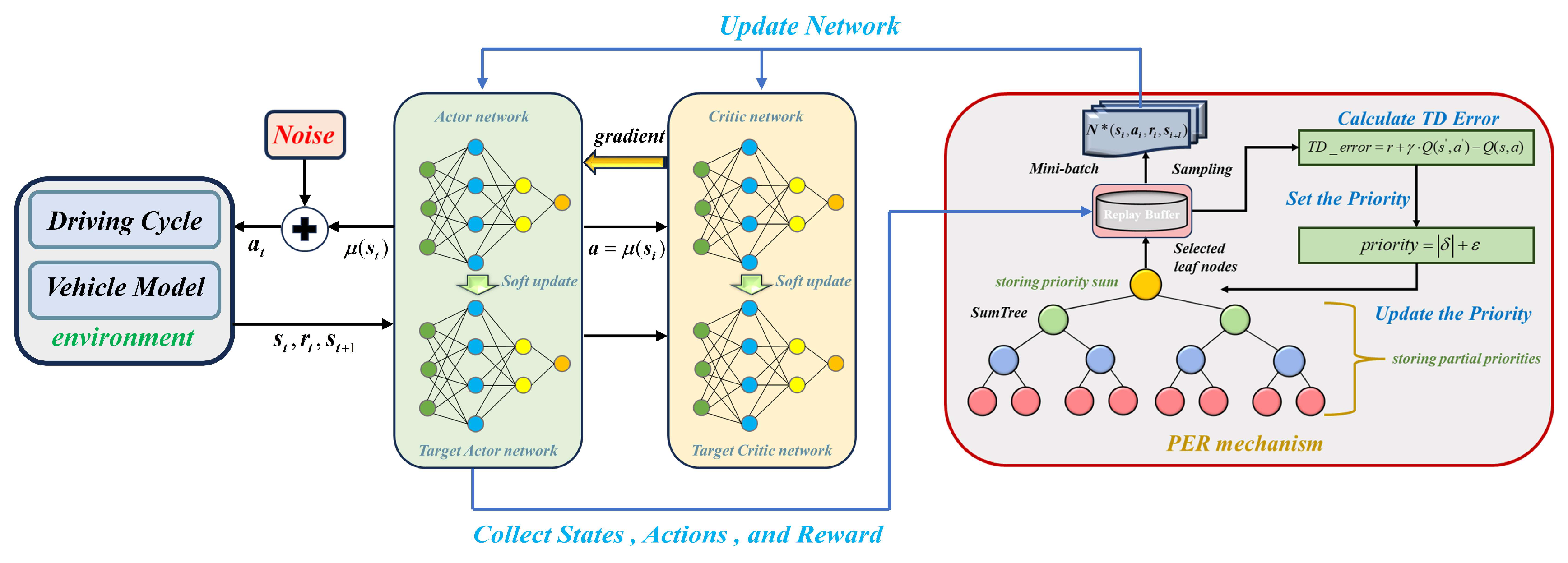
• Combination of prioritized experience replay (PER) with the traditional DDPG algorithm to form the PER–DDPG algorithm, which is used for training EMS of fuel cell vehicles.
• Integration of DRL with TL by transferring the experience data saved from the source task when training the target task, aiming to accelerate model convergence and enhance the EMS’s energy distribution performance.
• Employment of two different strategies for comparison to explore more appropriate TL methods: transfer all parameters of the neural network or transfer only part of the neural network parameters.

The structure of the remaining parts of this paper is shown in Figure 1.

2. Collection and Modeling for Fuel Cell Vehicles

2.1. Data Collection

The test vehicle (a manufacturer-specific 7-seat MPV hydrogen fuel cell vehicle) was instrumented with a CAN analyzer to monitor real-time operational parameters through the vehicle controller. As illustrated in Figure 1, data from the controller were transmitted via the CAN bus to an external receiver and ultimately stored on a computer. The power system architecture, characteristic curves, and vehicle-related parameters are detailed in Figure 2 and

Table 1. Main configuration of the FCHEV.

Items	Parameters	Value
Vehicle	Curb weight	2650 kg
	Tire radius	0.35 m
	Frontal area	3 m2
	Rolling resistance coefficient	0.013
	Air resistance coefficient	0.36
	Final drive ratio	9.5

, respectively.

2.2. Fuel Cell Vehicle Structure

Figure 2a illustrates the power system architecture and energy flow pathways of the fuel cell vehicle, comprising a fuel cell system, a DC/DC converter, an inverter (DC/AC), a traction battery, and an electric motor. Based on this configuration, the vehicle operates in four distinct modes [32]:

• Pure electric mode.
• Pure fuel cell mode.
• Hybrid mode.
• Regenerative braking mode.

2.3. Power System Model

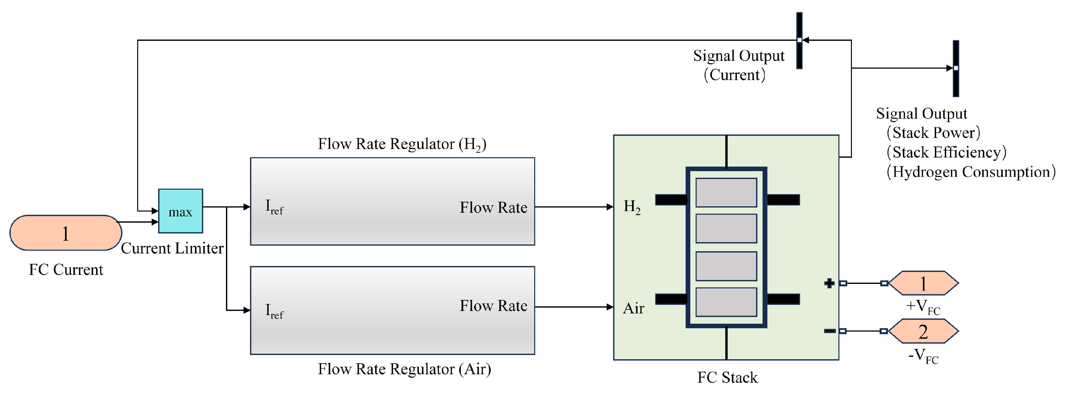
2.3.1. Fuel Cell Model

The fuel cell system serves as the primary power source of the vehicle, comprising a fuel cell stack and auxiliary components such as a hydrogen supply system, an air supply system, and others [33,34]. The fuel cell simulation system model is shown in Figure 3.

Figure 2b shows the efficiency and hydrogen consumption curves of the fuel cell. The fuel cell output power can be expressed as follows:

$$P_{fc}=U_{out}\cdot I_{st}\cdot {\eta }_{DC/DC}$$

(1)

where U_out is the output voltage of the fuel cell, I_st is the output current of the fuel cell stack, and η_DC/DC is the DC/DC converter efficiency.

The hydrogen consumption model of the fuel cell can be expressed as follows [35]:

$$m_{fc}={\displaystyle \frac{1}{LVH}}{\displaystyle \int \frac{P_{fc}}{{\eta }_{fc}{\eta }_{DC/DC}}}dt$$

(2)

where LVH is the low heating value of hydrogen and η_fc is the fuel cell efficiency.

2.3.2. Traction Battery Model

The traction battery acts as an auxiliary power source to compensate for the slow dynamic response of the fuel cell [36]. At the same time, it can store the surplus power from the fuel cell as well as the power generated by regenerative braking, thereby improving the vehicle’s range. Figure 2c illustrates the battery’s resistance and open-circuit voltage at different state-of-charge (SOC) levels. The SOC model of the battery can be expressed as follows:

$$SOC=\xi (P_{bat})={\displaystyle \frac{\sqrt{V_{OC}^2-4R_0{P}_{bat}}-V_{OC}}{2R_0{Q}_{bat}}}$$

(3)

where V_OC is the open-circuit voltage, R₀ is the internal resistance, Q_bat is the battery capacity, and P_bat is the battery power.

2.3.3. Motor Model

The electric motor is the driving device of the fuel cell vehicle with two operating modes, driving and regenerative braking, as shown in Figure 2d. The motor MAP diagram is the corresponding efficiency relationship of the motor at different speeds and torques. The model can be expressed as follows:

$$\left\{\begin{array}{l}{P}_m={\displaystyle \frac{{\omega }_m{T}_m{\eta }_m{\eta }_{DC/AC}}{9550}},T_m>0\\ P_m={\displaystyle \frac{{\omega }_m{T}_m}{9550{\eta }_m{\eta }_{DC/AC}}},T_m<0\end{array}\right.$$

(4)

where T_m is the torque, ω_m is the speed, η_m is the motor efficiency, and η_DC/AC is the inverter efficiency.

Table 2. Main parameters in the equation.

Parameter	Value	Unit
Uout	256–320	V
Ist	0–360	A
ηDC/DC	0.94	-
ηDC/AC	0.95	-
LVH	120	MJ/kg
Pfc	0–92	kW
ηfc	0–0.64	-
mfc	0–1.8783	g/s
VOC	280.8–305.36	V
R0 (discharging)	0.2808–0.9768	Ω
R0 (charging)	0.3364–0.9884	Ω
Qbat	13	kW·h
Pbat	0–104	kW
Tm	−310–310	N·m
ωm	0–16000	r/min
ηm	0.7–0.92	-

summarizes some constant values used in modeling.

3. Energy Management Strategies Based on PER–DDPG and Transfer Learning

3.1. The PER–DDPG Algorithm

In this study, a DDPG algorithm incorporating prioritized experience replay (PER) was designed, as shown in Figure 4. The core of the DDPG is an actor–critic architecture-based agent that interacts with the environment through states, actions, and rewards, aiming to maximize long-term rewards [37,38].

In DRL, samples are generated in chronological order, which can lead to correlations between them. To break this correlation, an experience replay mechanism is typically employed [39]. Specifically, data generated from the agent’s interactions with the environment are stored in a replay buffer. During training, a mini-batch of data is randomly sampled from the buffer to compute the loss function and update the model parameters. However, different samples do not share the same importance, and in traditional experience replay, all samples have an equal probability of being drawn, making it easy to overlook crucial experiences. PER is an improvement over traditional experience replay in that it prioritizes samples based on their importance, thus favoring experiences that contribute more to training. In this study, PER replaces the conventional experience replay in the DDPG, forming the PER–DDPG algorithm and improving the model’s training efficiency under complex operating conditions.

PER determines the importance of each sample based on the TD error. A larger TD error indicates a greater deviation between the model’s prediction and the actual sample, and therefore the sample is more valuable for training. The TD error is expressed as follows:

$$\mathrm{TD}\mathrm{error}=r+\gamma \cdot Q(s^{\prime },a^{\prime })-Q(s,a)$$

(5)

where r denotes the instantaneous reward, γ represents the discount factor, and Q (s′, a′) and Q (s, a) represent the Q-values of the target network and the main network in the DDPG algorithm, respectively.

The sampling probability is proportional to the TD error:

$$P_i={\displaystyle \frac{p_i^{\rho }}{{\Sigma }_k{p}_k^{\rho }}}$$

(6)

where P_i denotes the sampling probability of the ith sample, ρ_i is the TD error of the ith sample, and ρ is the prioritization factor.

The SumTree structure is a binary tree designed to improve the computational efficiency of PER [40]. In this structure, leaf nodes store the sample priority weights, while each parent node stores the sum of its child node values. Because PER changes the data distribution, it introduces bias and can increase instability. Therefore, importance sampling weights are required to correct the effect of different samples on the model:

$${\omega }_i={({\displaystyle \frac{1}{N\cdot P(i)}})}^{\beta }$$

(7)

where ω_i denotes the weight of the ith sample, N denotes the capacity of the experience replay buffer, and β denotes the bias correction parameter.

3.2. Algorithm Setting

In reinforcement learning algorithms, the choice of state variables and action variables determines the optimization goal of the algorithm. State variables describe the current interaction environment. Specifically, in the EMS studied in this paper, the state variables include the SOC, vehicle speed, acceleration, fuel cell power, and battery power, defined as follows:

$$\mathrm{state}=\left\{SOC,v,acc,P_{fc},P_{bat}\right\}$$

(8)

Since the fuel cell is the main power source of the vehicle analyzed in this paper, the action variable was defined as follows:

$$\mathrm{action}=\left\{P_{fc}\right\}$$

(9)

The optimization objectives of the EMS in this study were to reduce the hydrogen consumption of the fuel cell and keep the state of charge within a reasonable range. Therefore, the reward function was set as follows:

$$\mathrm{reward}=-\{\alpha [fuel(t)]+\beta {[so{c}_{ref}-soc(t)]}^n\}$$

(10)

where α and β are the respective weight parameters of the two objectives, fuel(t) represents the hydrogen consumption of the fuel cell, and SOC_ref is the reference value for maintaining the target SOC. Based on the relevant literature and experimental test results, the parameters α and β were set to 1 and 350, respectively [41].

3.3. Transfer Learning

A neural network is capable of extracting features from data. Based on these features, we combined transfer learning (TL) with the PER–DDPG algorithm to enable the model to converge quickly and improve performance when training the EMS under new working conditions. The principle of transfer learning is shown in Figure 5: the source domain was used as a pre-training model, which achieved convergence by training on multiple driving conditions and saved the weights and bias parameters in the hidden layer of the actor–critic network. The target domain reused the parameters of the source domain network to assist in initializing the model during training, and then fine-tuned the model according to the new task to adapt to the new data features. The TL model can be expressed using the following equation:

$${\theta }_T={\theta }_S+\Delta \theta$$

(11)

where θ_T represents the target domain parameters, θ_S denotes the source domain parameters, and Δθ denotes the fine-tuned update of the target domain.

In the PER–DDPG algorithm, the hidden layers of the actor–critic structure consist of three fully connected layers, with the number of neurons being 200, 100, and 50, respectively. The detailed structure of the hidden layers is shown as follows:

$$\mathrm{Actor}\left\{\begin{array}{l}{h}_1=\mathrm{Re}LU(w_{1}s+b_1)\\ h_2=\mathrm{Re}LU(w_2{h}_1+b_2)\\ h_3=\mathrm{Re}LU(w_3{h}_2+b_3)\end{array}\right.$$

(12)

$$\mathrm{Critic}\left\{\begin{array}{l}{h}_1=\mathrm{Re}LU(w_{1s}s+w_{1a}a+b_1)\\ h_2=\mathrm{Re}LU(w_2{h}_1+b_2)\\ h_3=\mathrm{Re}LU(w_3{h}_2+b_3)\end{array}\right.$$

(13)

where h represents the neural network layer, ReLU is the activation function, and w and b represent the weight and bias, respectively. Each layer in the hidden layers is responsible for a different task: the first layer is responsible for extracting basic information from each feature dimension of the input state s; the second layer captures the correlations between state variables based on this information; and the third layer performs higher-level abstraction and refinement on the features extracted by the second layer, providing highly integrated feature support for the output layer [42]. To explore the optimal transfer learning strategy, we designed two methods: transferring all parameters of the three hidden layers or transferring only the parameters of the first two hidden layers while reinitializing the third layer’s features with the neural network in the target domain. The rationale for this selection is that the first two layers of the network extract fundamental, general-purpose features that improve generalization in the target task. In contrast, the third layer encodes higher-level, task-specific decision logic; transferring its parameters can impede policy re-adaptation in the target task and result in negative transfer. The hyperparameter settings for the source and target domains are shown in

Table 3. Hyperparameter configuration.

Parameters	Source Domain	Target Domain
Episode	500	100
Replay buffer size	50,000	50,000
Learning rate of the actor network	0.001	0.0009
Learning rate of the critic network	0.001	0.0009
Reward discount	0.9	0.9
Batch size	64	64

.

4. Results and Discussion

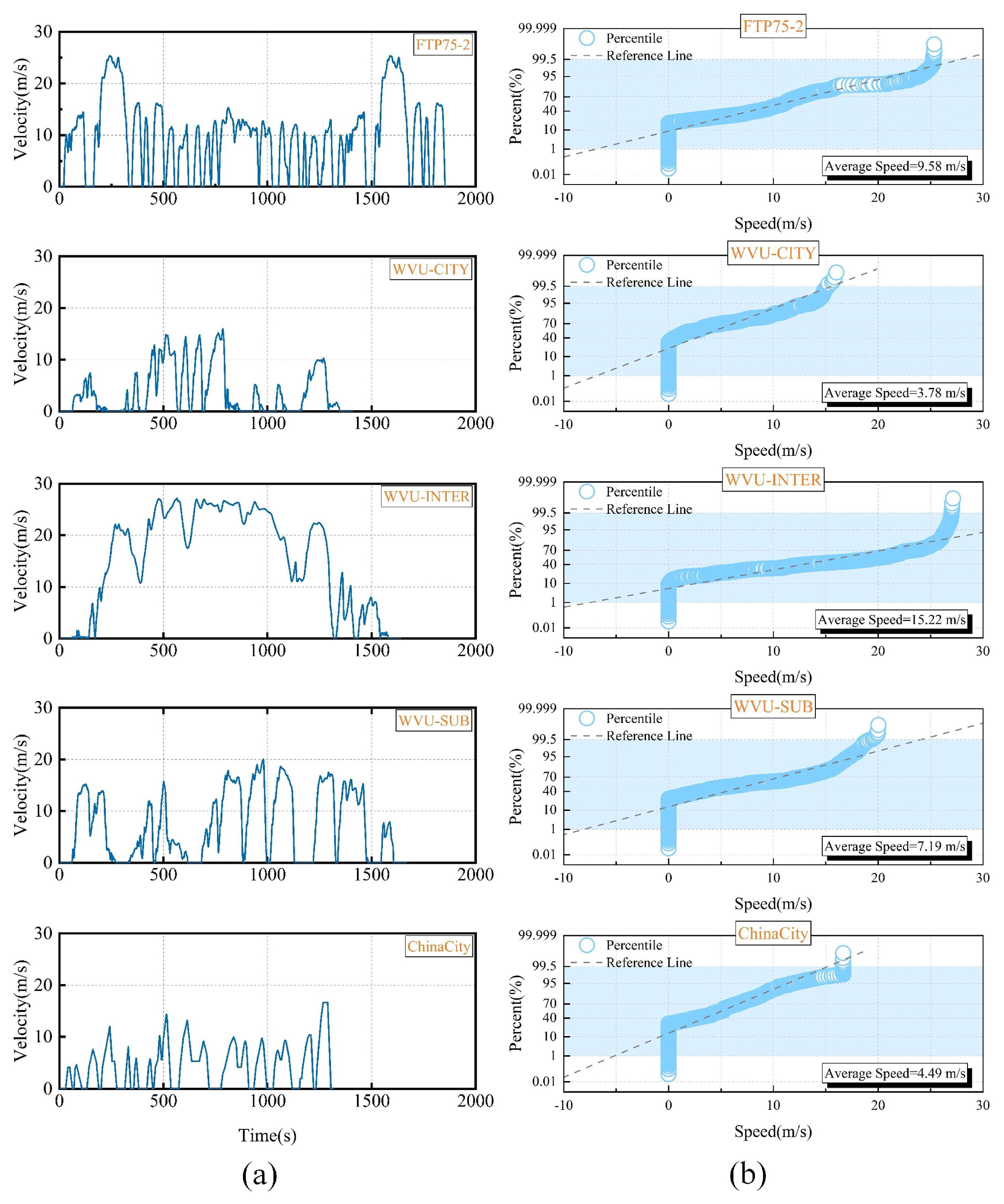
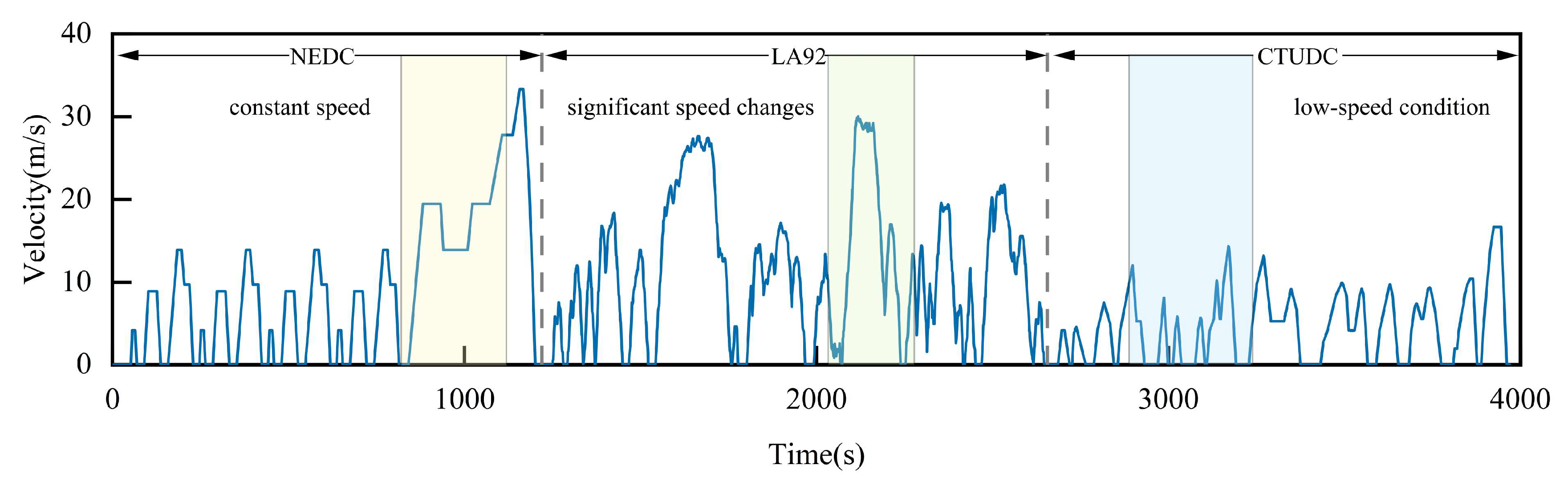
4.1. Driving Cycles

In order to ensure excellent generalization of the target domain model, five typical driving cycles (shown in Figure 6) were selected for the source domain. These cycles cover three different speed variation scenarios: urban, suburban, and peri-urban. The specific training procedure was as follows: first, an identifier was assigned to each of the five driving cycles; next, in each episode, one of these cycles was randomly selected for training; finally, once the model was converged, the corresponding neural network parameters were saved.

Table 4. Attributes of driving cycles.

Driving Cycles	Characteristics	Average Speed	Scenario
FTP75-2	Frequent stops and starts	9.58 m/s (34.49 km/h)	Urban peak traffic
WVU-CITY	More rapid acceleration	3.78 m/s (13.61 km/h)	Urban driving
WVU-INTER	Smooth speed changes	15.22 m/s (54.79 km/h)	Intercity driving condition
WVU-SUB	Stable speed, fewer stops	7.19 m/s (25.88 km/h)	Suburban driving
ChinaCity	Low speed	4.49 m/s (16.16 km/h)	Congested urban traffic

demonstrates the various attributes of the five driving cycles trained in the source domain, which include the characteristics of the driving cycles, the average speed, and the application scenarios.

Figure 7 shows the target domain driving cycle, which consists of the NEDC, the LA92, and the CTUDC. The NEDC, or the New European Driving Cycle, represents European urban and suburban driving scenarios, characterized by long periods of driving at a constant speed and overall smooth driving conditions. The LA92 is based on actual road driving data from the Los Angeles area and includes more sections with sharp acceleration and deceleration, simulating a complex driving environment. The CTUDC is a typical urban driving cycle in China. Due to severe urban road congestion, the average speed in this driving condition is low, and start–stop driving is more frequent. This hybrid driving cycle is more complex, overlapping with the source domain driving cycles, but also quite different, and can more comprehensively evaluate the effect of TL.

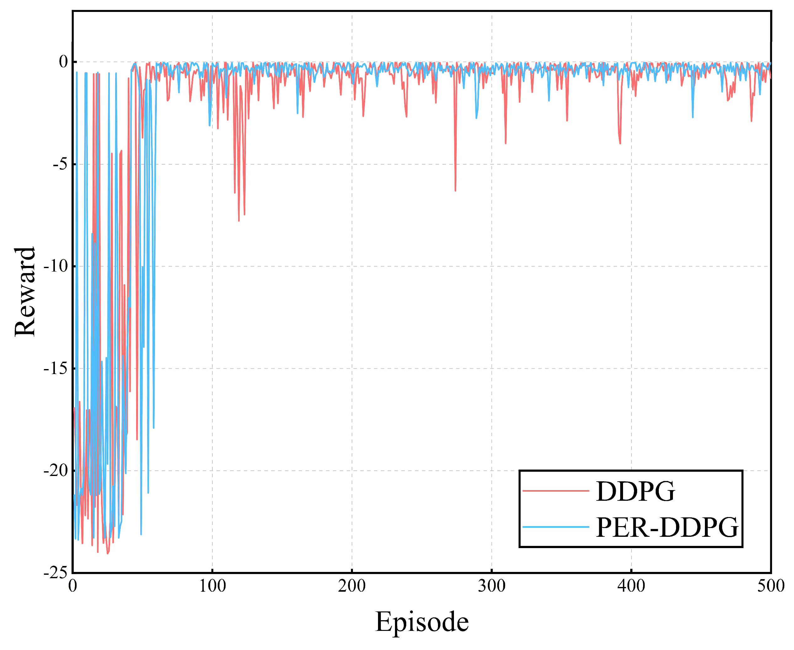
4.2. Training Conditions of the Source Domain

In order to achieve good results with TL, it is essential to first train a well-performing model for the source domain. In this study, the selected driving cycles were relatively complex, making the training process more challenging, so efficient algorithms were required. As shown in Figure 8, the source domain model was trained using both the traditional DDPG algorithm and the PER–DDPG algorithm. From the figure, it can be seen that the DDPG algorithm performed poorly in training the model, with not only a lower average reward, but also frequent large fluctuations, indicating slow convergence and poor stability. In contrast, the performance of the PER–DDPG was significantly better than that of the DDPG, with the reward stabilizing earlier, and smaller frequency and amplitude of fluctuations after convergence. Overall, PER significantly improved the performance of the DDPG, showing stronger adaptability in complex environments.

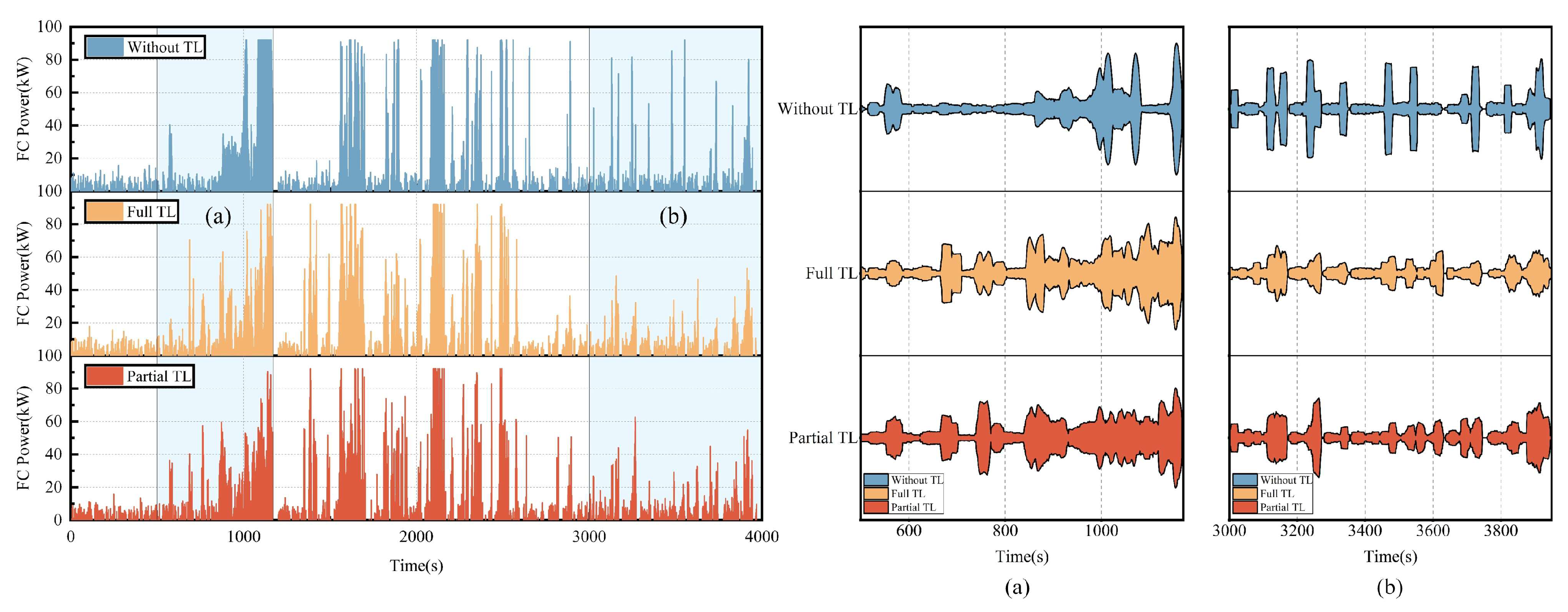
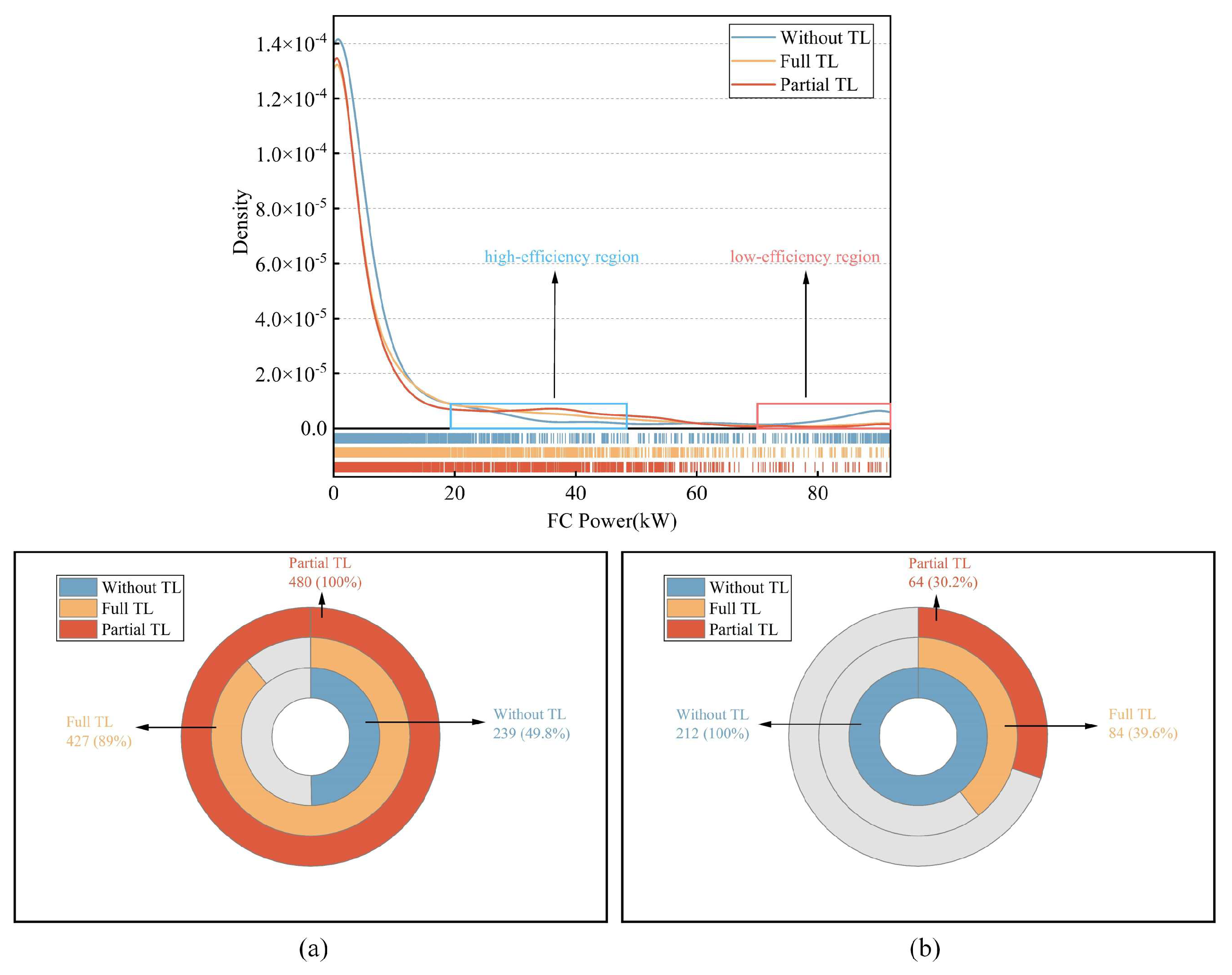
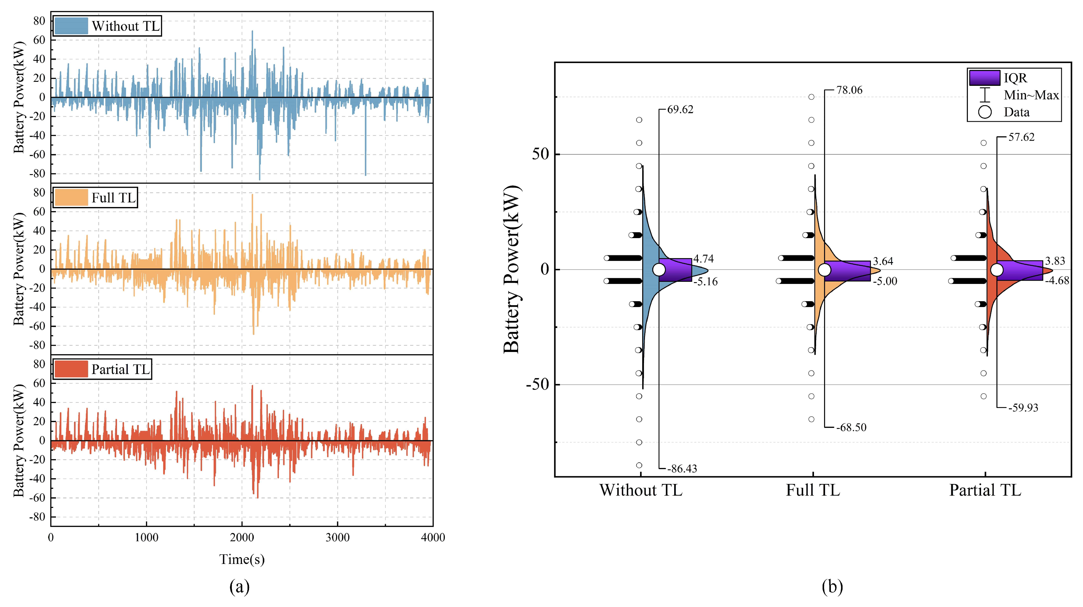
4.3. Power Distribution of Energy Sources in the Target Domain

In order to verify the effect of transfer learning, we took an EMS without transfer learning as a benchmark and compared it with two transfer learning methods. In the following, the EMS without transfer learning is referred to as Without TL, the strategy of transferring three layers of neural network parameters is referred to as Full TL, and the strategy of transferring the first two layers of neural network parameters is referred to as Partial TL.

The power output of the fuel cell under the target-domain mixed driving cycle with the three strategies is shown in Figure 9. Figure 9a,b uses kite charts to depict fuel cell power; the larger the chart’s area, the higher the power output. Under the Without TL strategy, the power of the fuel cell fluctuated drastically and frequently switched between low-power and high-power operating states. According to the dynamic characteristics of the fuel cell power output shown in Figure 9a,b, the adaptability of the EMS to complex operating conditions was significantly enhanced with TL, and the fuel cell operated more smoothly. Specifically, Figure 9a shows the effect of the EMS on the fuel cell output power when entering the high-speed condition from the low-speed condition in the NEDC. The transition of fuel cell power from low to high was very unsmooth under the Without TL strategy, whereas with the use of TL, the EMS was able to gradually increase the fuel cell power in accordance with the speed change of the condition. Figure 9b shows the effect of the EMS on the fuel cell output power after entering the CTUDC. The Without TL strategy performed poorly in this driving cycle, and it was difficult to adapt to the low-speed urban conditions, where the fuel cell frequently operated in the high-power range. The two strategies using TL could still operate smoothly under complex working conditions due to the reuse of parameters from the source domain task.

Table 5. STD and CV of the fuel cell power under the three strategies.

Strategy	STD	CV
Without TL	21,450.7	2.22
Full TL	17,305.63	1.92
Partial TL	17,112.07	1.89

shows the standard deviation and the coefficient of variation (the ratio of the standard deviation to the mean) of the fuel cell power under the three strategies, which are used to measure the absolute and relative fluctuations of the data, respectively. The expression is as follows:

$$\mathrm{STD}=\sqrt{{\displaystyle \frac{{\displaystyle \sum _{i=1}^n{(x_i-\mu )}^2}}{n}}}$$

(14)

$$\mathrm{CV}={\displaystyle \frac{STD}{\mu }}$$

(15)

where μ denotes the mean value.

From the data in Table 5, it can be seen that with the use of TL, the fuel cell power output was relatively smoother and the occurrence rate of large fluctuations was lower. The Partial TL strategy had the best performance, with the standard deviation (STD) and coefficient of variation (CV) decreasing by 20.26% and 14.86%, respectively.

Fuel cells working in the low-efficiency interval for a long time not only increase hydrogen consumption, but also accelerate the catalyst aging rate, which adversely affects the lifetime. From Figure 10, it can be seen that the working point distribution of the fuel cell was optimized after using TL, and both TL strategies reduced the number of working points of the fuel cell in the low-efficiency interval. At the same time, they allowed the fuel cell to work in the high-power interval in more scenarios. Under the Without TL strategy, the number of working points of the fuel cell in the low-efficiency interval was 212, and the number of working points in the high-efficiency interval was 239. With transfer learning applied, the number of working points in the low-efficiency interval reduced by 60.38% and 69.81% for the Full TL and Partial TL policies, respectively, and the number of working points in the high-efficiency interval increased by 78.66% and 100.84%, respectively.

Figure 11 shows the performance of the three strategies when the traction battery was outputting energy. Under the Without TL strategy, the traction battery’s charging and discharging power ranged from −86.43 kW to 69.62 kW, and the overcharge problem was more serious. Moreover, the interquartile range (IQR) of the battery power was from −5.16 kW to 4.74 kW, which is much larger than that of the other two strategies, indicating that the traction battery’s operating state was not stable enough and the operating point distribution was relatively dispersed. If the traction battery operates in this state for a long time, it will increase heat loss and adversely affect its lifespan. Under the Full TL strategy, the traction battery’s charge and discharge power ranged from −68.5 kW to 78.06 kW. By using transfer learning, the problem of overcharging in this strategy was optimized, but there were several problems with the output power at the operating points being too high. The IQR range of the Full TL strategy was from −5 kW to 3.64 kW, which is narrower than that of the Without TL strategy and improved stability. The Partial TL strategy had the best energy distribution effect for the traction battery, with a balanced charge and discharge distribution. The power range was from −59.93 kW to 57.62 kW, and the IQR range was from −4.68 kW to 3.83 kW, which showed the best stability performance.

4.4. SOC Maintenance Performance in the Target Domain

Maintaining the SOC within a moderate range and allowing the battery to charge and discharge in a low-resistance state can effectively reduce battery degradation. In this study, the target SOC was set to 0.6, and the initial SOC was 0.65. Figure 12a illustrates the temporal variation of the SOC. It can be seen from the figure that the effectiveness of SOC maintenance under the Without TL strategy was the worst, with a large deviation from the target value. Under the two TL strategies, the SOC was maintained close to the target value. The evaluation system in Figure 12b consists of the following indicators:

$$\left\{\begin{array}{l}MAE={\displaystyle \frac{1}{n}}{\displaystyle \sum _{i=1}^n\left|y_i-\overline{y_i}\right|}\\ MSE={\displaystyle \frac{1}{n}}{\displaystyle \sum _{i=1}^n(y_i-\overline{y_i}}{)}^2\\ RMSE=\sqrt{{\displaystyle \frac{1}{n}}{\displaystyle \sum _{i=1}^n(y_i-\overline{y_i}}{)}^2}\\ MRE={\displaystyle \frac{1}{n}}{\displaystyle \sum _{i=1}^n\left|\frac{y_i-\overline{y_i}}{y_i}\right|}\\ Bias={\displaystyle \frac{1}{n}}{\displaystyle \sum _{i=1}^n(\overline{y_i}}-y_i)\end{array}\right.$$

(16)

Among them, MAE indicates the average absolute error between the actual value and the target value; MSE is the mean of the squared sum of the errors; RMSE is the square root of MSE; and MRE measures the relative proportion of the error to the target value. The lower the value of these four indicators, the smaller the error. Bias represents the average deviation, and the closer the value is to 0, the smaller the deviation. As can be seen from Figure 12b and the data in

Table 6. Data of various indicators under different strategies.

Indicator	Without TL	Full TL	Partial TL	Full TL Improvement	Partial TL Improvement
MAE	0.0116	0.0074	0.0070	36.21%	39.66%
MSE	0.00025	0.00019	0.00017	24.00%	32.00%
RMSE	0.0158	0.0138	0.0134	12.66%	15.19%
MRE	0.0187	0.0119	0.0111	36.36%	40.64%
Bias	−0.0114	−0.0073	−0.0069	35.96%	39.47%

, after using TL, all errors were significantly reduced, and the Partial TL strategy performed better than the Full TL strategy. In the bias indicator, the Partial TL strategy also showed a value closer to 0 than the Full TL strategy.

4.5. Model Training Efficiency and Hydrogen Consumption in the Target Domain

The average reward of the target domain model training is shown in Figure 13a. The Without TL strategy, which did not use TL, converged in the 44th round. After using TL, the model training efficiency was significantly improved. Under the Partial TL strategy, the initial reward value was higher than that of Without TL and Full TL, and it reached a converged state in the 18th round. Under the Full TL strategy, the model converged in the 20th round, which is slightly less effective than Partial TL. The two methods, Full TL and Partial TL, improved the convergence speed by 54.55% and 59.09%, respectively.

As shown in Figure 13b,c, the hydrogen consumption of the fuel cell vehicle decreased after using transfer learning. After model convergence, the average hydrogen consumption was 596.24 g under the Without TL strategy, 570.15 g under the Full TL strategy, a decrease of 2.74%, and 564.64 g under the Partial TL strategy, a decrease of 3.69%. Based on the above comparison, it can be concluded that the overall performance of the EMS under the Partial TL strategy was the best.

5. Conclusions

This paper proposes an energy management strategy that combines deep reinforcement learning and transfer learning and applies it to hydrogen fuel cell vehicles. The implementation method of this strategy is as follows: first, a source domain model is trained using data from multiple driving cycles, and the experience (neural network parameters) learned from the source domain is saved. When training the target domain model, these parameters are reused to improve the convergence speed and energy distribution effectiveness of the target domain model. Compared to other deep reinforcement learning-based energy management strategies, the proposed strategy effectively avoids the shortcomings of poor generalization. The key conclusions and contributions are as follows:

1. Prioritized experience replay (PER) can effectively enhance the training efficiency of reinforcement learning algorithms. The PER–DDPG algorithm used in this paper significantly outperformed the traditional DDPG algorithm in training the source domain model.

2. In the TL task addressed in this paper, the source task was trained on five driving cycles, whereas the target task was trained on a single hybrid driving cycle. Although there were similarities, significant differences also existed. For instance, the source task typically used cycles with a total driving time of no more than 2000 s, while the target task employed a continuous, more complex cycle lasting close to 4000 s. These discrepancies introduced a risk of negative transfer. A comparison of two TL methods confirms that transferring parameters from higher-level neural network layers readily induces negative transfer. Therefore, when applying transfer learning to scenarios in which the source and target tasks differ substantially, the transfer of highly abstract features should be avoided.

3. Using a strategy without transfer learning and reinitializing the model as a benchmark, transfer learning strategies showed significant improvements in the following aspects: model convergence speed increased by 59.09%; fuel cell and battery power output stability improved, and the working point distribution became more reasonable. The number of working points of the fuel cell in the low-efficiency range decreased by 69.81%, while the number of working points in the high-efficiency range increased by 100.84%; hydrogen consumption decreased by 3.69%; SOC maintenance effectiveness improved, and the target SOC error (MAE) decreased by 39.66%.

For the fuel cell to operate stably and efficiently, its operating temperature needs to be controlled. Therefore, the thermal management system is an important guarantee for the fuel cell. In addition to the fuel cell, the traction battery likewise requires precise temperature control. The thermal management system uses the fuel cell’s waste heat to warm the battery until it reaches its optimal operating temperature; when the temperature rises too high, it adjusts the coolant valve opening to hasten heat rejection. Future research will apply deep learning and transfer learning to the thermal management system.

References

1. Pramuanjaroenkij, A.; Kakac, S. The fuel cell electric vehicles: The highlight review. Int. J. Hydrogen Energy 2023, 48, 9401–9425. [Google Scholar] [CrossRef]
2. Song, H.; Liu, C.; Moradi Amani, A.; Gu, M.; Jalili, M.; Meegahapola, L.; Yu, X.; Dickeson, G. Smart optimization in battery energy storage systems: An overview. Energy AI 2024, 17, 100378. [Google Scholar] [CrossRef]
3. Li, X.; Ye, T.; Meng, X.; He, D.; Li, L.; Song, K.; Jiang, J.; Sun, C. Advances in the Application of Sulfonated Poly(Ether Ether Ketone) (SPEEK) and Its Organic Composite Membranes for Proton Exchange Membrane Fuel Cells (PEMFCs). Polymers 2024, 16, 2840. [Google Scholar] [CrossRef] [PubMed]
4. Deng, K.; Liu, Y.; Hai, D.; Peng, H.; Löwenstein, L.; Pischinger, S.; Hameyer, K. Deep reinforcement learning based energy management strategy of fuel cell hybrid railway vehicles considering fuel cell aging. Energy Convers. Manag. 2022, 251, 115030. [Google Scholar] [CrossRef]
5. Luca, R.; Whiteley, M.; Neville, T.; Shearing, P.R.; Brett, D.J.L. Comparative study of energy management systems for a hybrid fuel cell electric vehicle- A novel mutative fuzzy logic controller to prolong fuel cell lifetime. Int. J. Hydrogen Energy 2022, 47, 24042–24058. [Google Scholar] [CrossRef]
6. Chen, B.; Ma, R.; Zhou, Y.; Ma, R.; Jiang, W.; Yang, F. Co-optimization of speed planning and cost-optimal energy management for fuel cell trucks under vehicle-following scenarios. Energy Convers. Manag. 2024, 300, 117914. [Google Scholar] [CrossRef]
7. Meng, X.; Sun, C.; Mei, J.; Tang, X.; Hasanien, H.M.; Jiang, J.; Fan, F.; Song, K. Fuel cell life prediction considering the recovery phenomenon of reversible voltage loss. J. Power Sources 2025, 625, 235634. [Google Scholar] [CrossRef]
8. Sun, X.; Fu, J.; Yang, H.; Xie, M.; Liu, J. An energy management strategy for plug-in hybrid electric vehicles based on deep learning and improved model predictive control. Energy 2023, 269, 126772. [Google Scholar] [CrossRef]
9. Lu, D.G.; Yi, F.Y.; Hu, D.H.; Li, J.W.; Yang, Q.Q.; Wang, J. Online optimization of energy management strategy for FCV control parameters considering dual power source lifespan decay synergy. Appl. Energy 2023, 348, 121516. [Google Scholar] [CrossRef]
10. Dai-Duong, T.; Vafaeipour, M.; El Baghdadi, M.; Barrero, R.; Van Mierlo, J.; Hegazy, O. Thorough state-of-the-art analysis of electric and hybrid vehicle powertrains: Topologies and integrated energy management strategies. Renew. Sustain. Energy Rev. 2020, 119, 109596. [Google Scholar]
11. Hou, S.; Gao, J.; Zhang, Y.; Chen, M.; Shi, J.; Chen, H. A comparison study of battery size optimization and an energy management strategy for FCHEVs based on dynamic programming and convex programming. Int. J. Hydrogen Energy 2020, 45, 21858–21872. [Google Scholar] [CrossRef]
12. Oladosu, T.L.; Pasupuleti, J.; Kiong, T.S.; Koh, S.P.J.; Yusaf, T. Energy management strategies, control systems, and artificial intelligence-based algorithms development for hydrogen fuel cell-powered vehicles: A review. Int. J. Hydrogen Energy 2024, 61, 1380–1404. [Google Scholar] [CrossRef]
13. Zhang, X.; Wang, X.; Yuan, P.; Tian, H.; Shu, G. Optimizing hybrid electric vehicle coupling organic Rankine cycle energy management strategy via deep reinforcement learning. Energy AI 2024, 17, 100392. [Google Scholar] [CrossRef]
14. Jia, C.C.; Zhou, J.M.; He, H.W.; Li, J.W.; Wei, Z.B.; Li, K.A. Health-conscious deep reinforcement learning energy management for fuel cell buses integrating environmental and look-ahead road information. Energy 2024, 290, 130146. [Google Scholar] [CrossRef]
15. Jia, C.; He, H.; Zhou, J.; Li, J.; Wei, Z.; Li, K.; Li, M. A novel deep reinforcement learning-based predictive energy management for fuel cell buses integrating speed and passenger prediction. Int. J. Hydrogen Energy 2025, 100, 456–465. [Google Scholar] [CrossRef]
16. Lee, W.; Jeoung, H.; Park, D.; Kim, T.; Lee, H.; Kim, N. A Real-Time Intelligent Energy Management Strategy for Hybrid Electric Vehicles Using Reinforcement Learning. IEEE Access 2021, 9, 72759–72768. [Google Scholar] [CrossRef]
17. Han, X.; He, H.; Wu, J.; Peng, J.; Li, Y. Energy management based on reinforcement learning with double deep Q-learning for a hybrid electric tracked vehicle. Appl. Energy 2019, 254, 113708. [Google Scholar] [CrossRef]
18. Du, G.; Zou, Y.; Zhang, X.; Guo, L.; Guo, N. Energy management for a hybrid electric vehicle based on prioritized deep reinforcement learning framework. Energy 2022, 241, 122523. [Google Scholar] [CrossRef]
19. Zhang, J.; Jiao, X.; Yang, C. A Double-Deep Q-Network-Based Energy Management Strategy for Hybrid Electric Vehicles under Variable Driving Cycles. Energy Technol. 2021, 9, 2000770. [Google Scholar] [CrossRef]
20. Tan, H.; Zhang, H.; Peng, J.; Jiang, Z.; Wu, Y. Energy management of hybrid electric bus based on deep reinforcement learning in continuous state and action space. Energy Convers. Manag. 2019, 195, 548–560. [Google Scholar] [CrossRef]
21. Hu, B.; Li, J. A Deployment-Efficient Energy Management Strategy for Connected Hybrid Electric Vehicle Based on Offline Reinforcement Learning. IEEE Trans. Ind. Electron. 2022, 69, 9644–9654. [Google Scholar] [CrossRef]
22. Wu, J.D.; Wei, Z.B.; Li, W.H.; Wang, Y.; Li, Y.W.; Sauer, D.U. Battery Thermal- and Health-Constrained Energy Management for Hybrid Electric Bus Based on Soft Actor-Critic DRL Algorithm. IEEE Trans. Ind. Inform. 2021, 17, 3751–3761. [Google Scholar] [CrossRef]
23. Liu, R.; Wang, C.; Tang, A.H.; Zhang, Y.Z.; Yu, Q.Q. A twin delayed deep deterministic policy gradient-based energy management strategy for a battery-ultracapacitor electric vehicle considering driving condition recognition with learning vector quantization neural network. J. Energy Storage 2023, 71, 108147. [Google Scholar] [CrossRef]
24. Hu, Y.; Xu, H.; Jiang, Z.; Zheng, X.; Zhang, J.; Fan, W.; Deng, K.; Xu, K. Supplementary Learning Control for Energy Management Strategy of Hybrid Electric Vehicles at Scale. IEEE Trans. Veh. Technol. 2023, 72, 7290–7303. [Google Scholar] [CrossRef]
25. Wu, C.C.; Ruan, J.G.; Cui, H.H.; Zhang, B.; Li, T.Y.; Zhang, K.X. The application of machine learning based energy management strategy in multi-mode plug-in hybrid electric vehicle, part I: Twin Delayed Deep Deterministic Policy Gradient algorithm design for hybrid mode. Energy 2023, 262, 125084. [Google Scholar] [CrossRef]
26. Li, M.; Liu, H.; Yan, M.; Wu, J.; Jin, L.; He, H. Data-driven bi-level predictive energy management strategy for fuel cell buses with algorithmics fusion. Energy Convers. Manag. X 2023, 20, 100414. [Google Scholar] [CrossRef]
27. Zhou, J.; Liu, J.; Xue, Y.; Liao, Y. Total travel costs minimization strategy of a dual-stack fuel cell logistics truck enhanced with artificial potential field and deep reinforcement learning. Energy 2022, 239, 121866. [Google Scholar] [CrossRef]
28. Lee, H.; Song, C.; Kim, N.; Cha, S.W. Comparative Analysis of Energy Management Strategies for HEV: Dynamic Programming and Reinforcement Learning. IEEE Access 2020, 8, 67112–67123. [Google Scholar] [CrossRef]
29. Wang, K.; Yang, R.; Zhou, Y.; Huang, W.; Zhang, S. Design and Improvement of SD3-Based Energy Management Strategy for a Hybrid Electric Urban Bus. Energies 2022, 15, 5878. [Google Scholar] [CrossRef]
30. Lian, R.; Tan, H.; Peng, J.; Li, Q.; Wu, Y. Cross-Type Transfer for Deep Reinforcement Learning Based Hybrid Electric Vehicle Energy Management. IEEE Trans. Veh. Technol. 2020, 69, 8367–8380. [Google Scholar] [CrossRef]
31. Lu, D.; Hu, D.; Wang, J.; Wei, W.; Zhang, X. A data-driven vehicle speed prediction transfer learning method with improved adaptability across working conditions for intelligent fuel cell vehicle. IEEE Trans. Intell. Transp. Syst. 2025; Early Access. [Google Scholar]
32. Jouda, B.; Al-Mahasneh, A.J.; Abu Mallouh, M. Deep stochastic reinforcement learning-based energy management strategy for fuel cell hybrid electric vehicles. Energy Convers. Manag. 2024, 301, 117973. [Google Scholar] [CrossRef]
33. Yan, M.; Li, G.; Li, M.; He, H.; Xu, H.; Liu, H. Hierarchical predictive energy management of fuel cell buses with launch control integrating traffic information. Energy Convers. Manag. 2022, 256, 115397. [Google Scholar] [CrossRef]
34. Jia, C.; Zhou, J.; He, H.; Li, J.; Wei, Z.; Li, K.; Shi, M. A novel energy management strategy for hybrid electric bus with fuel cell health and battery thermal- and health-constrained awareness. Energy 2023, 271, 127105. [Google Scholar] [CrossRef]
35. Hu, D.; Wang, Y.; Li, J. Energy saving control of waste heat utilization subsystem for fuel cell vehicle. IEEE Trans. Transp. Electrif. 2023, 10, 3192–3205. [Google Scholar] [CrossRef]
36. Xie, S.; Hu, X.; Xin, Z.; Brighton, J. Pontryagin’s Minimum Principle based model predictive control of energy management for a plug-in hybrid electric bus. Appl. Energy 2019, 236, 893–905. [Google Scholar] [CrossRef]
37. Li, J.; Wu, X.; Hu, S.; Fan, J. (Eds.) A Deep Reinforcement Learning Based Energy Management Strategy for Hybrid Electric Vehicles in Connected Traffic Environment. In Proceedings of the 6th IFAC Conference on Engine Powertrain Control, Simulation and Modeling (E-COSM), Tokyo, Japan, 23–25 August 2021. [Google Scholar]
38. Zheng, C.; Zhang, D.; Xiao, Y.; Li, W. Reinforcement learning-based energy management strategies of fuel cell hybrid vehicles with multi-objective control. J. Power Sources 2022, 543, 231841. [Google Scholar] [CrossRef]
39. Tang, X.; Zhou, H.; Wang, F.; Wang, W.; Lin, X. Longevity-conscious energy management strategy of fuel cell hybrid electric Vehicle Based on deep reinforcement learning. Energy 2022, 238, 121593. [Google Scholar] [CrossRef]
40. Gao, Z.; Gao, Y.; Hu, Y.; Jiang, Z.; Su, J. (Eds.) Application of Deep Q-Network in Portfolio Management. In Proceedings of the 5th IEEE International Conference on Big Data Analytics (ICBDA), Xiamen, China, 8–11 May 2020. [Google Scholar]
41. Zhu, Z.; Lin, K.; Jain, A.K.; Zhou, J. Transfer learning in deep reinforcement learning: A survey. IEEE Trans. Pattern Anal. Mach. Intell. 2023, 45, 13344–13362. [Google Scholar] [CrossRef]
42. Wang, K.; Wang, H.; Yang, Z.; Feng, J.; Li, Y.; Yang, J.; Chen, Z. A transfer learning method for electric vehicles charging strategy based on deep reinforcement learning. Appl. Energy 2023, 343, 121186. [Google Scholar] [CrossRef]
Figure 1. Structure of the paper.
Energies 18 02192 g001
Figure 2. Powertrain structure and characteristics. (a) The powertrain structure of the FCHEV. (b) FC characteristic. (c) Traction battery performance. (d) Motor map.
Energies 18 02192 g002
Figure 3. Fuel cell system simulation model.
Energies 18 02192 g003
Figure 4. PER–DDPG algorithm structure.
Energies 18 02192 g004
Figure 5. Principle of transfer learning.
Energies 18 02192 g005
Figure 6. Relevant information of driving cycles. (a) Source domain driving cycles. (b) Speed distribution.
Energies 18 02192 g006
Figure 7. Target domain driving cycle.
Energies 18 02192 g007
Figure 8. Source domain model training performance.
Energies 18 02192 g008
Figure 9. Comparison of fuel cell power output under different strategies. (a,b) Dynamic characteristics of the fuel cell power output.
Energies 18 02192 g009
Figure 10. Fuel cell operating point density distribution. (a) Number of operating points in the high-efficiency region. (b) Number of operating points in the low-efficiency region.
Energies 18 02192 g010
Figure 11. Traction battery performance. (a) Traction battery charging and discharging power. (b) Traction battery energy distribution.
Energies 18 02192 g011
Figure 12. SOC maintenance performance and error. (a) SOC variation curve. (b) Error between the SOC and the target value.
Energies 18 02192 g012
Figure 13. Training performance and hydrogen consumption analysis. (a) Average reward curve. (b) Hydrogen consumption curve. (c) Average hydrogen consumption after convergence.
Energies 18 02192 g013