Learning and Characterizing Chaotic Attractors of a Lean Premixed Combustor

Abstract

This paper is about the characteristics of and a method to recognize the onset of limit cycle thermoacoustic oscillations in a gas turbine-like combustor with a premixed turbulent methane/air flame. Information on the measured time series data of the pressure and the OH* chemiluminescence is acquired and postprocessed. This is performed for a combustor with variation in two parameters: fuel/air equivalence ratio and combustor length. It is of prime importance to acknowledge the nonlinear dynamic nature of these instabilities. A method is studied to interpret thermoacoustic instability phenomena and assess quantitatively the transition of the combustor from a stable to an unstable regime. In this method, three-phase portraits are created on the basis of data retrieved from the measured acoustics and flame intensity in the laboratory-scale test combustor. In the path to limit cycle oscillation, the random distribution in the three-phase portrait contracts to an attractor. The phase portraits obtained when changing operating conditions, moving from the stable to the unstable regime and back, are analyzed. Subsequently, the attractor dimension is determined for quantitative analysis. On the basis of the trajectories from the stable to unstable and back in one run, a study is performed of the hysteresis dynamics in bifurcation diagrams. Finally, the onset of the instability is demonstrated to be recognized by the 0-1 criterion for chaos. The method was developed and demonstrated on a low-power atmospheric methane combustor with the aim to apply it subsequently on a high-power pressurized diesel combustor.

1. Introduction

For power generation and propulsion, combustion of gaseous or liquid fuels in gas turbine engine combustors will remain important for decades to come in view of the high efficiency and power density. In the path of transition to sustainable fuels, methane and diesel/kerosene/jet fuel will be replaced by hydrogen, ammonia, and sustainable aviation fuel. The challenges related to their combustion will, however, remain. The emission of nitric oxides will still be an issue, and the drive to reduce them will continue. This is laid down in the Paris Agreement in 2015 [1], whose main goal is to achieve a decrease of 2 °C in the global temperature due to a reduction in emissions of up to 25% in 2030 [2]. In addition, the need to reduce and control thermoacoustic oscillations also has to be faced. A method that was proven to be successful in the past for natural gas to reach this low NOx emission target is lean premixed combustion. It remains to be seen if this concept will be an option with new sustainable fuels. But for all fuels, the occurrence of thermoacoustic instabilities in lean premixed combustion has to be reckoned with. This paper presents a method to analyze and predict the onset of instability and predict a likely growth of amplitudes. This is performed for premixed methane combustion with the option to generalize this to other combustion concepts.

The flame in the combustor is a powerful thermoacoustic monopole source that can drive the acoustics in the combustor into a high-amplitude limit cycle oscillation. This can lead to destructive processes in the engine [3]. Being able to predict and understand these instabilities is a continuous challenge that calls for experimental work on combustion systems that are representative of gas turbine engine combustion chambers. The aim is to develop effective post-processing concepts of the data, allowing predictive methodologies to avoid thermoacoustic instabilities [4].

In experimental work, the so-called data-driven approach, a nonlinear time series analysis to study thermoacoustic instabilities, has been presented in the works of Gotoda et al. [5] and more recently by [6] studying a ducted premixed laminar flame; intermittency state in premixed combustion [7]; the multifractal signature of transition combustion dynamics in [8]; influence of variations in the input heat flux [9]; effect of blending methane with hydrogen [10]; and premixed swirling flames in [11,12]. They have pioneered in the nonlinear analysis of laboratory-scale combustors, mostly with laminar flow.

Studied were the high-amplitude oscillations and how the system goes from chaotic to non-chaotic behavior. How to identify and make a clean distinction of the stages at which the combustor behavior changes was shown. This can be when the composition of the fuel, the position of the flame, or the air-to-fuel ratio varies for a certain combustor. Most of the nonlinear analysis through three-phase portraits has been performed in the laminar regime, with operational airflows of Reynolds numbers of the order of 1000. More recently, refs. [10,11] presented nonlinear analysis of the combustion dynamics of methane/hydrogen mixtures. Ref. [10] worked at leaner conditions and Reynolds numbers of 19,000, air-to-fuel equivalence ratio of 1.8, and increasing the percentage of methane. The change from stable to limit cycle oscillations occurs as methane is more prominent in the mass fraction. A property of a deterministic system is that its evolution is fully determined, but its predictability is limited by the exponential growth of errors in the measurements [13]. The prediction of a chaotic time series can be approximated by the nonlinear functional mapping of the signal. This is by far not a new idea, as the initial chaotic time series prediction takes us back to 1987, where it was already known that chaotic fluid flows can generate state spaces onto an attractor of a few dimensions [14]. However, computational power and developments in the artificial intelligence umbrella have now opened a world of possibilities to process experimental nonlinear data and make predictions with it.

The present study aims at nonlinear treatment of pressure and OH-chemiluminescence time series retrieved from the combustor with two different geometries. The data in the time series is based on data from multiple wall-mounted pressure transducers and data from a photomultiplier tube. The thermoacoustic system, composed of the combustion chamber and the flame, is viewed as a black box. With the methodology introduced by Abarbanel [15], three-phase portraits are obtained From the obtained time series based on the computed system delay time and global embedding dimension [16]. The phase portraits were obtained for a variation in the operating parameters, where the system evolved from stable/chaotic to deterministic/unstable and back. The transition from chaotic to deterministic was observed by means of the 0-1 test. For all operating conditions, the fractal dimension of the phase portraits was established and the predictive capabilities for thermoacoustic oscillations were analyzed. This was all performed for a high Reynolds number flow with the combustion flow well in the turbulent regime. This differs from studying laminar combustion in that if you have laminar combustion, most of the heat release disturbances are coupled to the pressure; in turbulent combustion, on the contrary, the heat release is affected by the pressure and by the turbulent flow fluctuations. Therefore, pressure fluctuations and heat release are noisier. This method can be used on a small scale and at atmospheric pressure, as well as for larger flows and high pressure, because it is easy to use the time series of the dynamic data OH-chemiluminescence and, more importantly, the pressure. The method can be used identically in both cases. The present paper is organized as follows: In Section 2, the applied methodology is introduced as is the combustion system on which this was applied. The combustion system delivered varied operating conditions data in terms of pressure transducer and photomultiplier time series. The behavior of the combustion system shows a bifurcation in the transition from stable to unstable operation. This is presented in Section 3. The nonlinear behavior of the combustion dynamics is analyzed by means of a phase space construction in Section 4. In Section 5, the 0-1 test for chaos is investigated to see if the transition from stable combustion dynamics with small growth rate to limit cycle oscillations is related to a switch from chaotic to deterministic behavior. If this can be used to predict the onset of limit cycle oscillations is explored. Finally, in Section 6, the conclusions and takeaway of the paper are summarized.

2. Methodology and Experimental Set up

In this section, first the methodology followed to investigate the nature of limit cycle oscillations is lined out. Subsequently, the combustor that is used to provide the data is presented. Since this is about thermoacoustic oscillations, the data obtained are time series of pressure samples and photomultiplier samples. The target of this study was to explore the unstable behavior of a combustor with a turbulent air inlet flow and turbulent flame. First, the time series are observed using a conventional Fourier transformation to reveal the spectral content of the signals. The combustor can operate either in a stable or unstable mode, with a well-reproduceable transition with a change in equivalence ratio. The oscillation amplitude distribution changes in a very characteristic way in the transition, and this is analyzed. This transition of amplitude distribution can be mapped in a bifurcation diagram, revealing the change in the combustion oscillations behavior.

More is to be learned from the obtained data time series by more advanced data processing. To this end, a phase space reconstruction is made of the data to observe the possible motion of the system to a lower-dimensional attractor. The presence of such an attractor would indicate chaotic system behavior switching to deterministic. Therefore, for all operation conditions, the 0-1 test for chaos is performed, it is and investigated if this will serve as a precursor for instability in this turbulent premixed combustor.

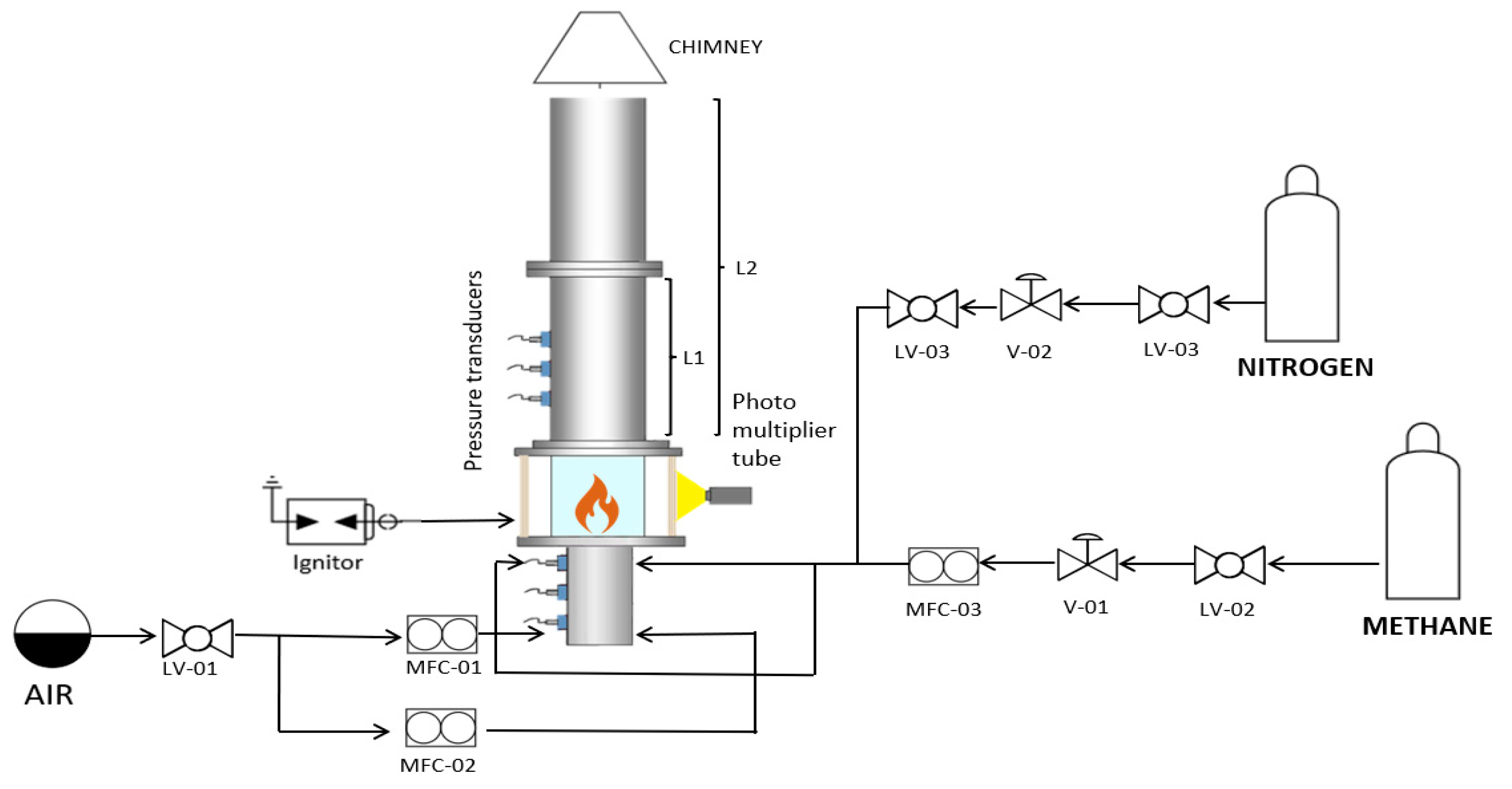
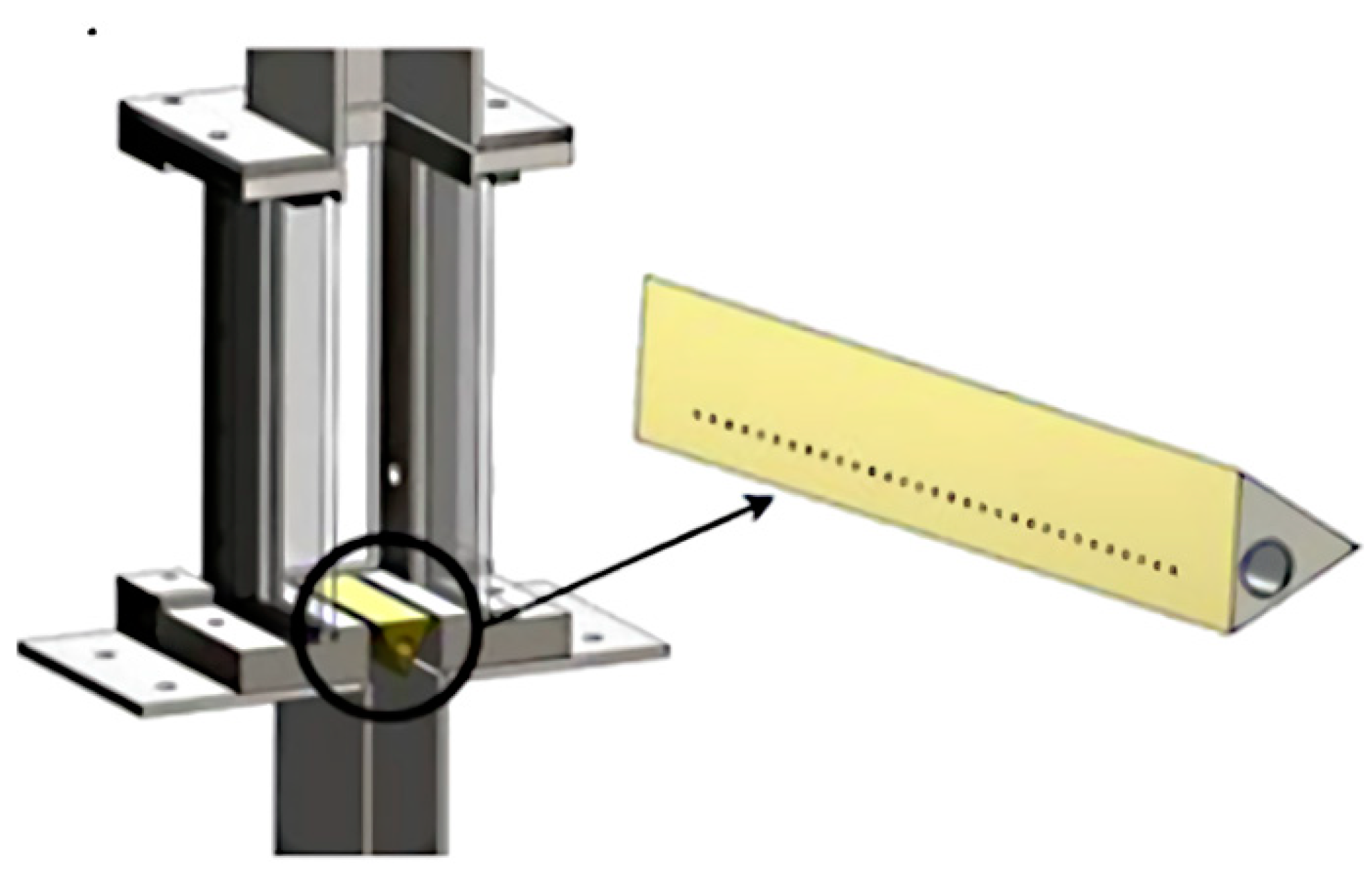
2.1. Experimental Set up

For the studies presented, an available combustion system was used. This was the combustor developed and built in the LIMOUSINE project. Figure 1 sketches the test rig layout and shows a detailed view of the burner geometry. This geometry consists of a triangular wedge holding the flame on the bluff body wake (Figure 2). The triangular wedge has a hollow body with 32 holes per face on both upstream-directing faces. Through these holes, methane fuel, supplied from both ends of the wedge, is injected into the airflow. Solenoid valves and mass flow controllers were controlled by a program run in LabView. This combustor burns stable at a lean fuel-to-air equivalence ratio but transits into limit cycle oscillation when the equivalence ratio is increased sufficiently close to. The air to the burner is supplied in a plenum that opens via the wedge passage into the combustion chamber that has a larger width. Since the airflow past the wedge has a high turbulence intensity, the methane fuel injected mixes fast, leading to a premixed methane/airflow into the combustor from each side of the wedge. The turbulent flame stabilizes on the recirculation area created by the boundary layer detachment at the two sharp downstream-facing edges of the wedge. The plenum has a length of 275 mm with a cross-section of 25 × 150 mm². (width × depth). The combustion chamber on top of the plenum has a length of 780 mm with a cross-section of 50 × 150 mm² (width × depth, L1 in Figure 1). The original length (L1) was defined as a quarter of the associated wavelength of the fundamental frequency under test, which is 50 Hz. In addition to this, it is similar to or lower than comparable lengths to other experimental combustors. The liner can be equipped with a liner extension that allows for an extra 610 mm of combustor length (L2 in Figure 1), giving an overall of 1610 mm full length. In the combustion chamber, four quartz windows are placed starting at the wedge position to allow optical access to the flame from all sides.

2.2. Instrumentation and Data Acquisition

Acoustic data are collected by 6 Kulite XTE 190M (±0.1% FSO BFSL (Typ.), ±0.5% FSO (Max.)) wall-mounted pressure transducers, 3 upstream and 3 downstream from the burner. Four thermocouples are installed, distributed over the length of the combustor. A Thorlabs PMM01 photomultiplier tube (Thorlabs Inc., Newton, NJ, USA, with quantum efficiency peak of 25%), with a bandpass filter of 310 nm mounted, was used to acquire the OH* chemiluminescence of the flame.

The signals are measured by National Instruments cards and a LabVIEW data acquisition program. The DAQ system (NI 9239) can read ±10 V signals at a maximum sample rate of 50,000 Hz simultaneously in all the (12) input channels. In the research performed here for each test, 3.2 s of data were obtained at a sample rate of 10,000 Hz. These sample parameters were chosen to be able to study pressure oscillations in the range of 50 to 800 Hz.

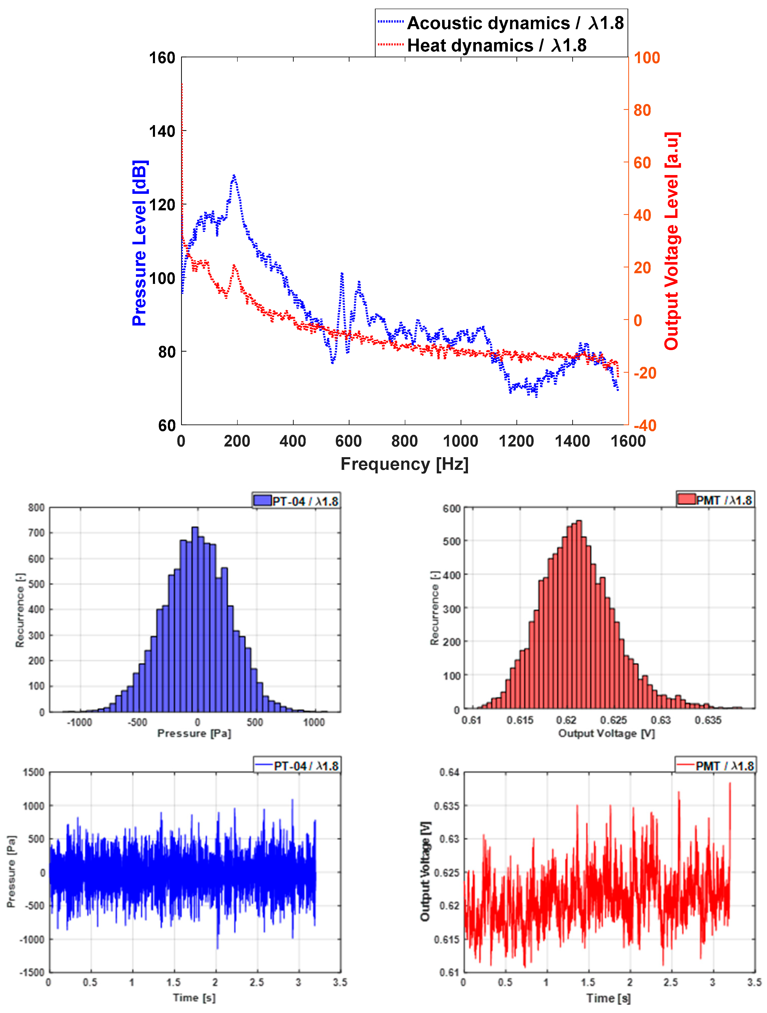
3. Analysis of Optics and Pressure Data

A series of experiments with lean combustion conditions is performed as follows, with the combustor at a nominal thermal power of 50 kW. The combustor is started near stoichiometric, and subsequently the airflow is quickly increased to reach an air factor of 1.9. In that situation the combustion process is stable and low-amplitude combustion noise is observed and driven by turbulence. Subsequently the air factor is decreased in steps of 0.1 (1.9 to 1.8 to 1.7…). The experiment is operated on the basis of three parameters: thermal power, air factor, and combustor length. The thermal power ranges between 20 kW and 80 Kw in order to have a turbulent flow. For practical reasons the rig is operated at 50 kW. The results were not sensitive to the thermal power. The air factor was in the range of 1 to 2 for lean combustion and to prevent blowoff. The combustor length was chosen with a view to the axial wavelength of the dominant frequencies. After every stepwise change in the airflow, pressure measurements are performed after the thermoacoustic system has become stationary. The air factor is decreased till well beyond the point the thermoacoustic system has become unstable and developed at a high amplitude limit cycle oscillation. The lowest air factor reached is 1.2, where the combination of high flame temperature and high amplitude pressure oscillations has reached the limit that the combustor can sustain for a brief time without being damaged. Subsequently the process is reversed, and the path back to an air factor of 1.9 is followed. This is in order to detect possible hysteresis in the nonlinear processes involved. The thermoacoustic system can switch between two characteristic states: stable low noise amplitude and limit cycle oscillation with high amplitude saturation.

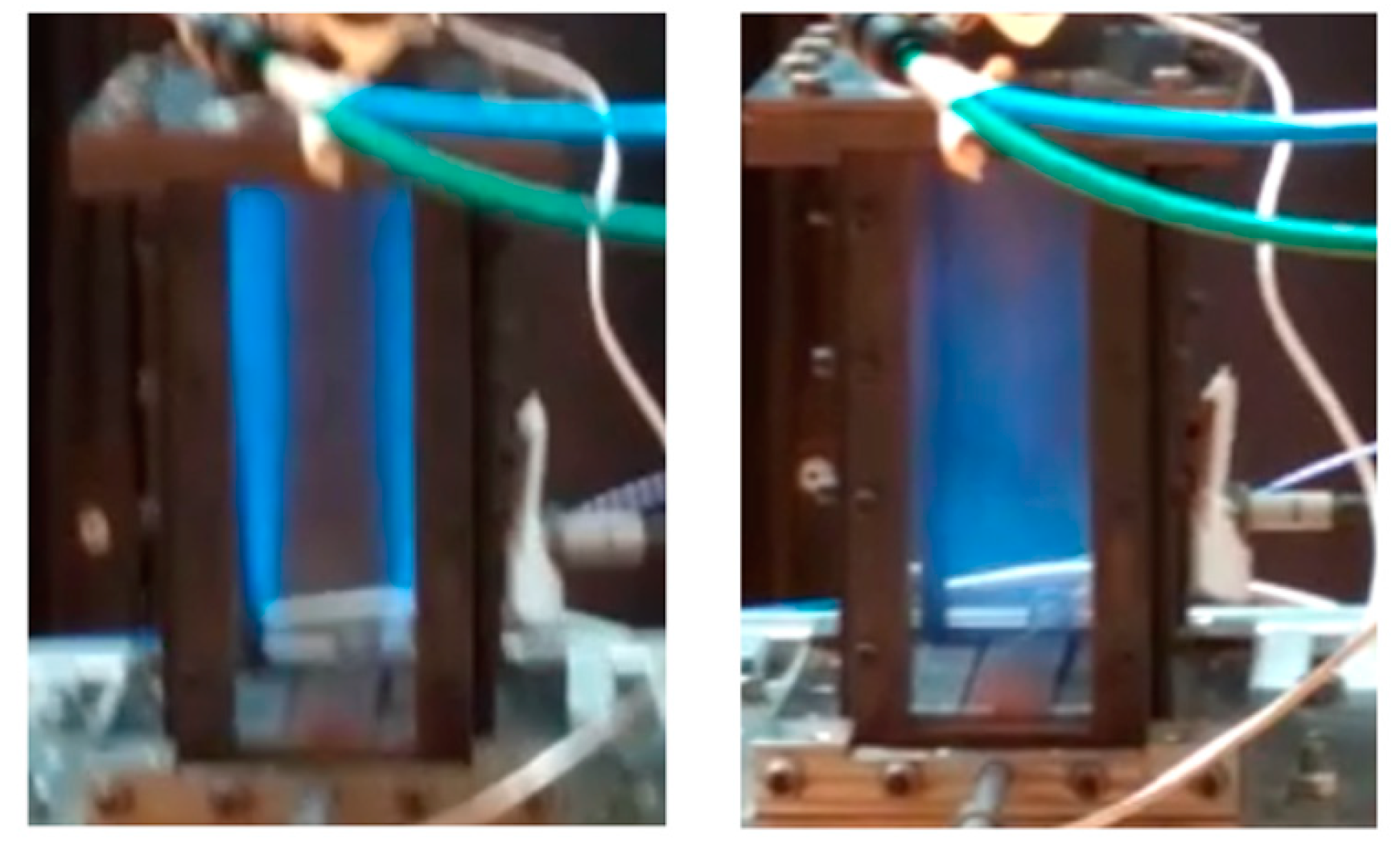
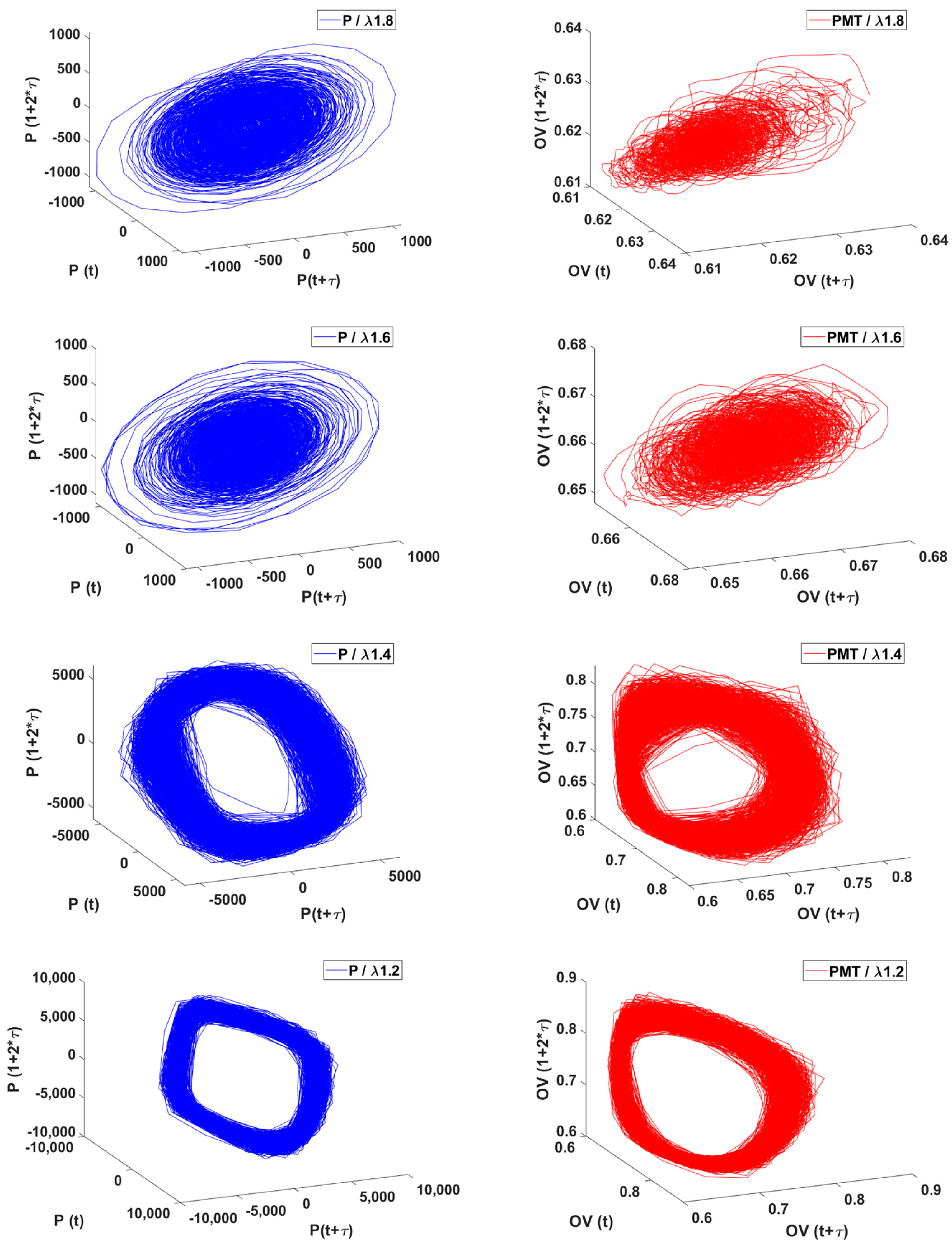
3.1. For the L1 Case (Original Length)

An optical snapshot viewed from the side of the combustor of the stable and the unstable case can be seen in Figure 3. For the air factor (λ) of 1.8 (left picture), it can be seen how the flame is totally divided in the two sides where the fuel holes are located. There is a long and thin flame that extends toward the optical window. On the right, we have a λ of 1.2, where we encountered limit cycle oscillations, shown as a compacted flame that anchors at the bluff body in its wake.

First, we look at the stable case, being the one with a higher air factor (λ = 1.8). Figure 4 shows the power spectrum in dB and related logarithmic units for both the acoustics and the rate of heat release. On both spectra, there are no resonant dominant frequencies observed. There is increased activity (130 dB) in the range of 50–300 Hz for the acoustic signal. The higher frequency amplitudes are below 100 dB. The signal histogram (middle) allows us to evaluate the amplitude distribution changes from a stable case to a transitional state and to an unstable situation. The time series (bottom), which for the case of the pressure is seen to heavily vary with time.

The stable mode pressure amplitude histogram at air factor 1.8 is observed to be a symmetric bell shape and symmetrically distributed on both sides of 0 amplitude with a maximum representation of low amplitudes and a decline of occurrence with increasing amplitude. The maximum amplitude with a very low occurrence is 400 Pa. For the OH* chemiluminescence case, the intensity time series vary strongly with time, and the histogram shows a bell-shaped distribution as well, balanced around mean chemiluminescence intensity, with its center slightly moved towards lower values.

Figure 5 shows a representative measured pressure time series of the limit cycle oscillation state and the frequency spectrum at air factor 1.2. The pressure amplitude is quite high and constant with time and indicates a saturation of the process. The spectrum for pressure oscillations shows a dominant peak of 160 dB at a frequency of 240 Hz. At this frequency the PMT signal (rate of heat release) also shows a very high peak.

Regarding the signal histograms, in the limit cycle mode the amplitude distribution has become flat with a strong emphasis on the high amplitudes. It can be concluded that the pressure amplitude distribution changes in a very characteristic way in the path to switch to the unstable/limit cycle mode. Regarding the OH* chemiluminescence, we see higher and constant values and a saturated signal. Nevertheless, the histogram shows a distribution of the intensity values most concentrated in low values and then a decay and a similar distribution for the higher intensities, with a slight peak around 0.83 (value as an arbitrary unit). And then a decrease. In the superposed spectra, a number of very dominant resonant frequencies can be observed. A main resonant frequency appears around 240 Hz at 165 dB. The structural mode is also observed and at a higher amplitude than in the stable mode (135 dB). Other resonant frequencies can be observed at 650 Hz, 800 Hz (140 dB), and 1400 Hz (120 dB). The characteristics of these two states and the system changes in the path for high-to-low air factors are explored next.

The cross-spectrum magnitude, phase, and coherence of the oscillations of gauge pressure and rate of heat release (measured by the chemiluminescence signal) are presented in Figure 6 for the cases of λ = 1.8 (dash-dot), 1.6 (dot), 1.4 (dash), and 1.2 (solid line). It can be seen that the coherence in all cases remains high up to about 1400 Hz, indicating a coupling of acoustics and rate of heat release fluctuations. From this figure the peak magnitude location and its phase are observed to analyze the nature of the oscillations. The Rayleigh equation for thermoacoustic instability predicts that if the phase of the peak magnitude is between −180 and 180 degrees, the rate of heat release fluctuations will amplify the pressure oscillations. In case the acoustic source term is larger than the damping and loss of acoustic energy, the growth rate will be positive, and a limit cycle may be reached. The two lean cases (λ = 1.8, 1.6) have a negative peak at 186 Hz for the first and 196 Hz for the second, both not significant and indicating that the signals are about 180 degrees out of phase. Hence, the oscillatory growth rate is negative or near zero.

In the close-to-stoichiometric air factor 1.4 case, there are three prominent peaks: the first, at 234 Hz and with a positive value, and the next ones have a negative value and are located at 467 Hz and 705 Hz. For the λ = 1.2 case, when the high-amplitude oscillations are happening, the cross spectrum shows the first peak at 246 Hz and a positive value. This indicates (and shows in the phase diagram) a phase difference between acoustics and rate of heat release fluctuations of about 0 degrees. This confirms the Rayleigh prediction of a positive growth rate and limit cycle oscillation. The next two peaks are at 493 Hz, with a positive value, and 740 Hz on a remarkably close value of the amplitude. There is a lower peak at 989 Hz. The coherence has a value of 1 that coincides with the more defined and larger amplitude peaks.

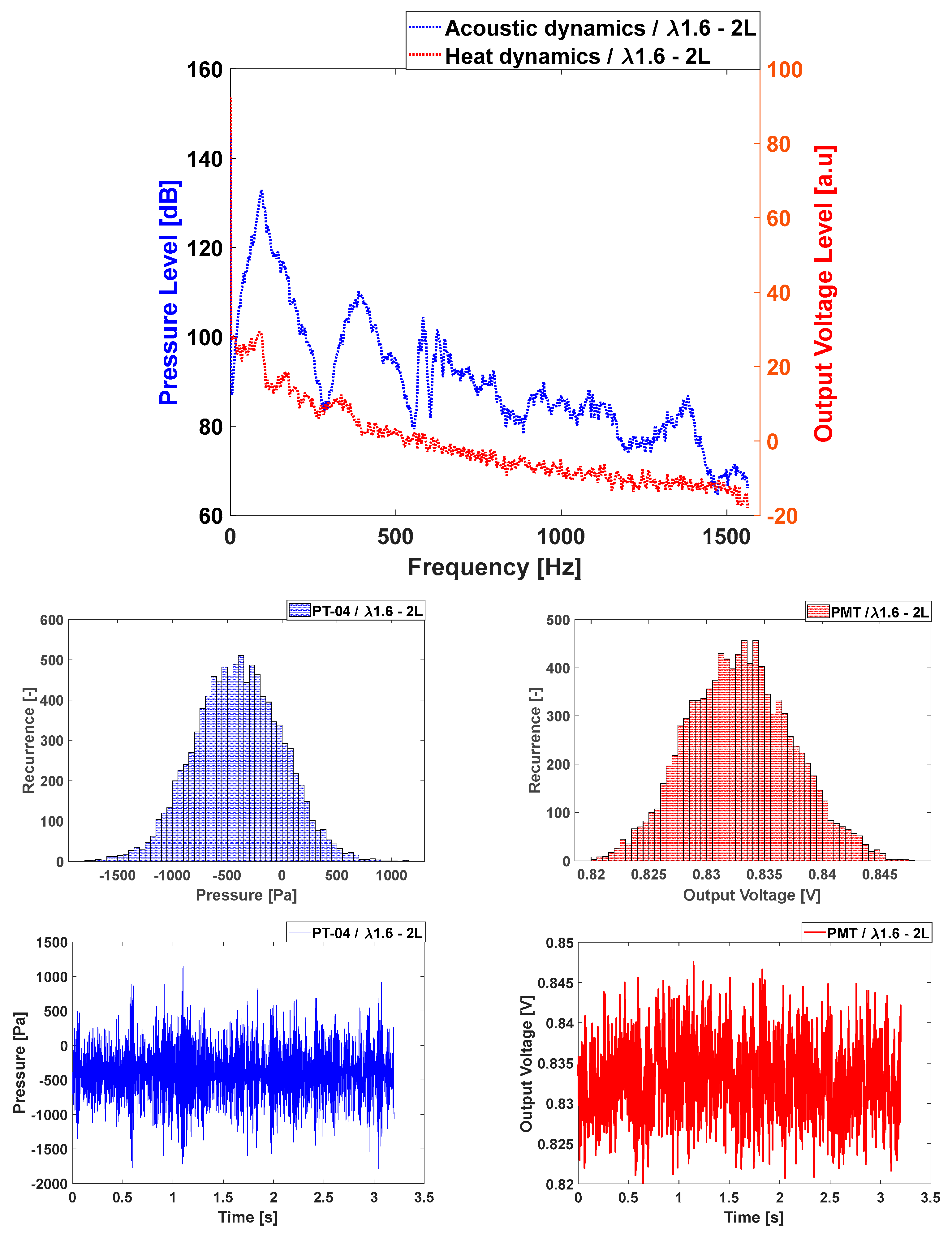
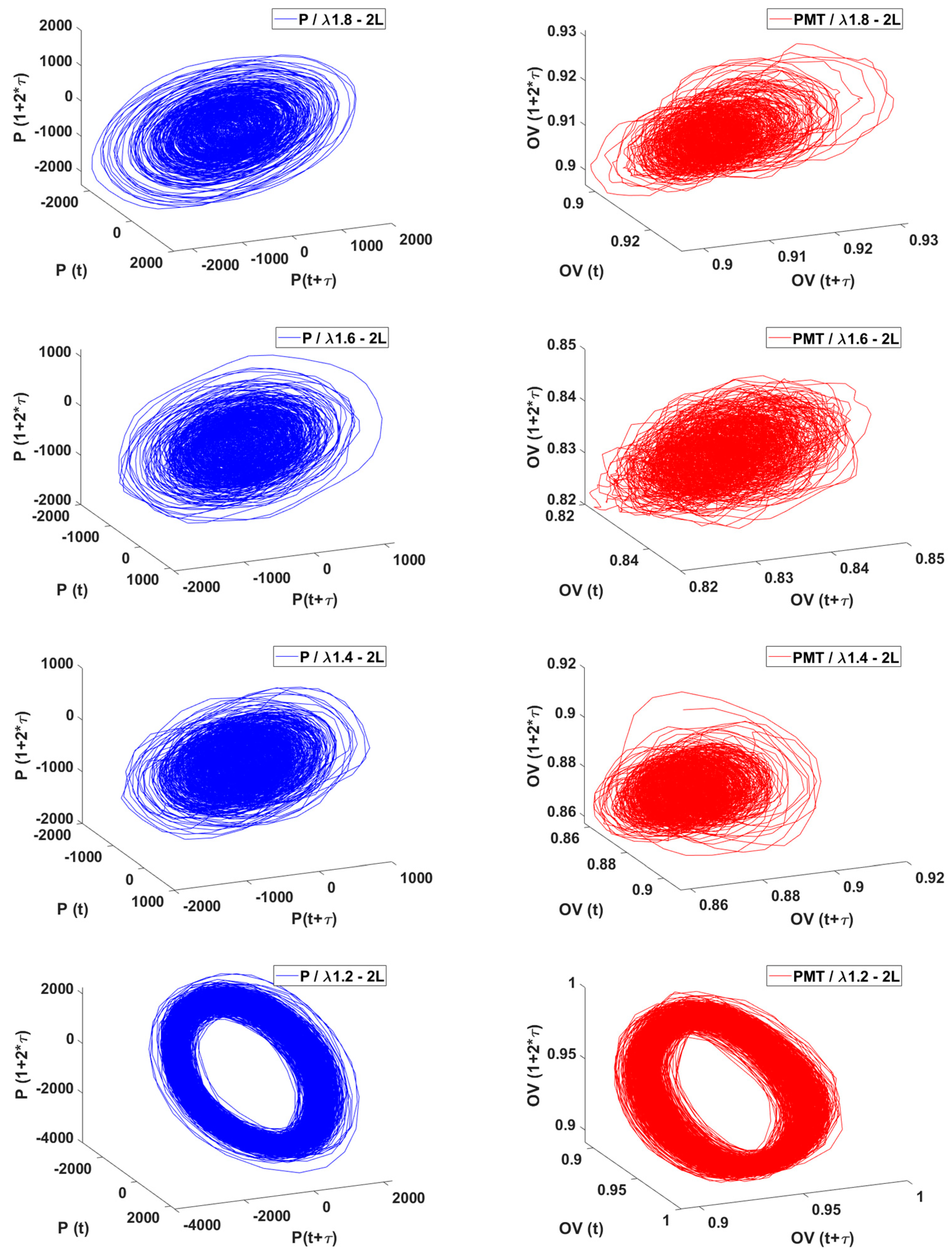
3.2. For the L2 Case (Double Length)

Subsequently, experiments are performed with the same combustor but at double length downstream of the burner deck, at a nominal power of 50 kW (0.99 g/s of methane) and the highest air–fuel equivalence ratio before reaching the lean blow-off. The experimental sequence was from λ = 1.8, 18.2 g/s of air, to λ = 1.2, 12.1 g/s of air, and back.

Figure 7 shows the pressure time series and the amplitude histogram for the stable case λ = 1.8. We again encounter a seemingly random varying pressure amplitude decreasing with frequency and a symmetrical gaussian shape for the amplitude distribution with most values concentrated in low amplitudes of less than 500 Pa. For the case of the PTM signal, for which raw data are presented, we see a randomly changing signal that tends to decrease its mean value with frequency, behavior that can also be appreciated in the amplitude distribution data histogram.

Figure 8 shows the pressure time series in an unstable case, reaching the limit cycle oscillation at this point, close to the stoichiometric combustion. The pressure amplitude is now high and constant; next to it, the histogram shows a “u” shape with peaks in high values of pressure. A similar response tendency can be observed for the PTM signal in its own unit rank.

Different from what was observed on the original combustor length. Where previously there was a clear transition regime that shared qualities of both unstable and stable regimes, for this geometry what happens is that in between the conditions of the stable and unstable regimes, the systems jump from one to the other.

Looking at the spectrums of both pressure and the PTM signal obtained by a Fourier for both λ = 1.8 and 1.2. For the first case, the pressure signal, there is a high dB around 100 Hz, and further than 200 Hz is not above 110 dB. The PTM signal does not show any excitation. For the second, λ = 1.2, at 162 Hz (of 155 dB for the pressure signal) and 327 Hz with an extra peak for the pressure signal at 585 Hz and 652 Hz, it is clear that both signals are coupled and correlated.

We can see that for the double-length case, the pressure peaks have displaced to lower frequencies, and they have a lower amplitude.

Meanwhile, the visual of the flame remains quite similar for both lengths.

In Figure 9 for the double length, the cross-spectrum magnitude, phase, and coherence of the pressure and the chemiluminescence are presented for λ = 1.8, 1.6, 1.4, and 1.2. It can be observed that for the λ = 1.6, we do not have an important peak in the cross spectrum. A high amplitude oscillation is not reached under these conditions. Apparently, a longer liner gives more damping to the acoustic waves, and reaching a self-excited oscillation requires a stronger thermoacoustic source term.

The λ = 1.8, 1.6, and 1.4 cases have a magnitude peak in 86 Hz, 146 Hz, and 95 Hz, respectively, all of them with values below zero. These cases have a phase shift of about 180 degrees and have a negative growth rate.

In the 1.2 case, there are two prominent magnitude peaks, at 165 Hz with a positive value and 467 Hz and 331 Hz with a negative one. Again, the coherence value validates the presence of the peaks.

3.3. Intermittent Case for L2

A particular feature of the studied combustor in the double-length version is that it presents a clearly intermittent case. Important observations of the intermittent case in a combustor and how the intermittency keeps being fed by the change in position in the flame related to its repositioning on the recirculation zones have been studied in experimental work [10]. When Figure 7 (stable) and Figure 8 (unstable) are compared to Figure 9 and Figure 10 for both lengths, this clearly shows the transition from the stable case, with lower amplitudes in the pressure and in the flame OH-chemiluminescence followed by sections of higher amplitude that repeat themselves over the time series of 3.2 s. When looking at the histograms, the distribution shape shows this tendency of having sections of big amplitude and maintaining these high values.

The spectra of both signals show important peaks, particularly at lower frequencies, mixed with a decay of the amplitude with frequency.

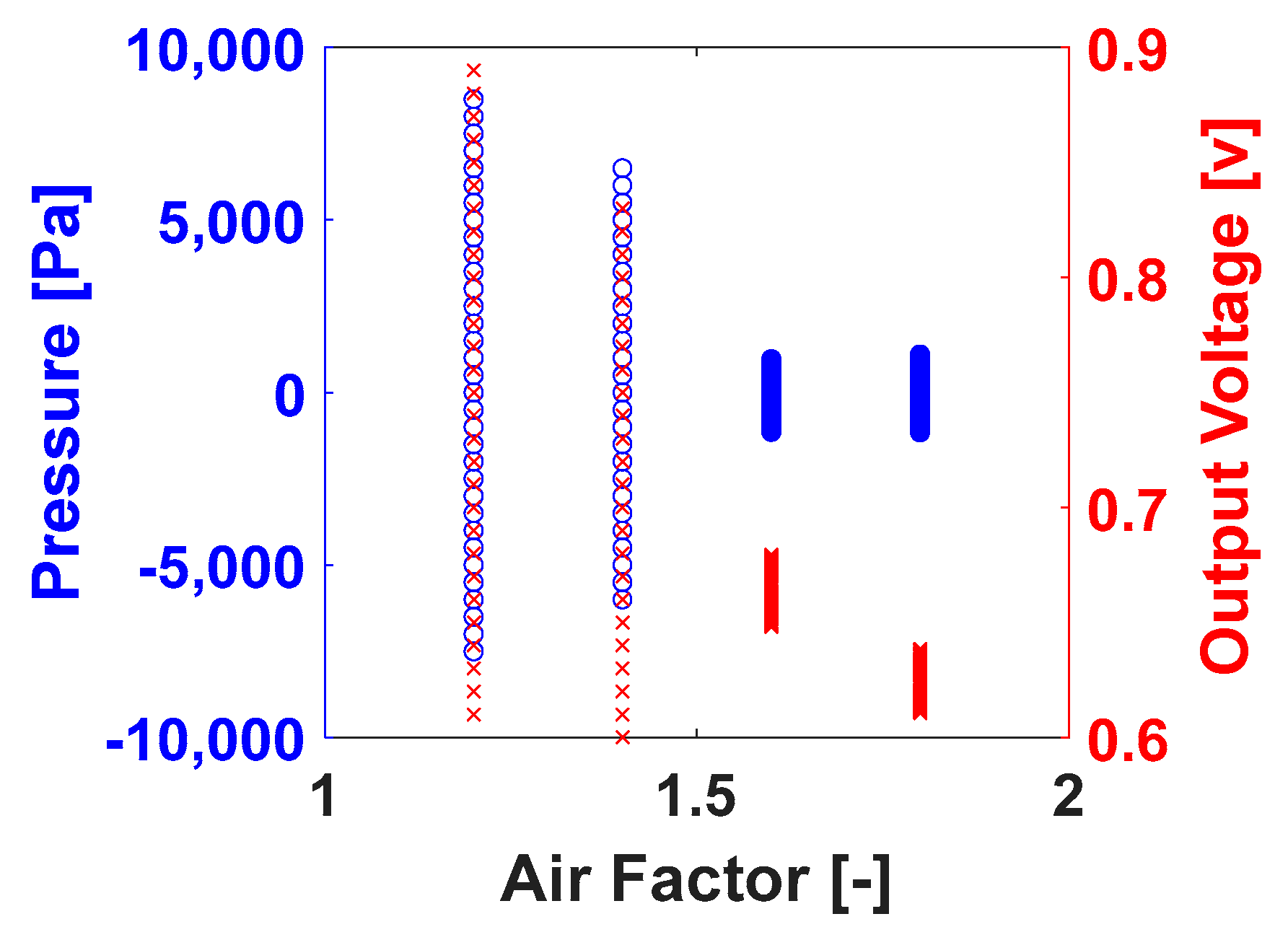
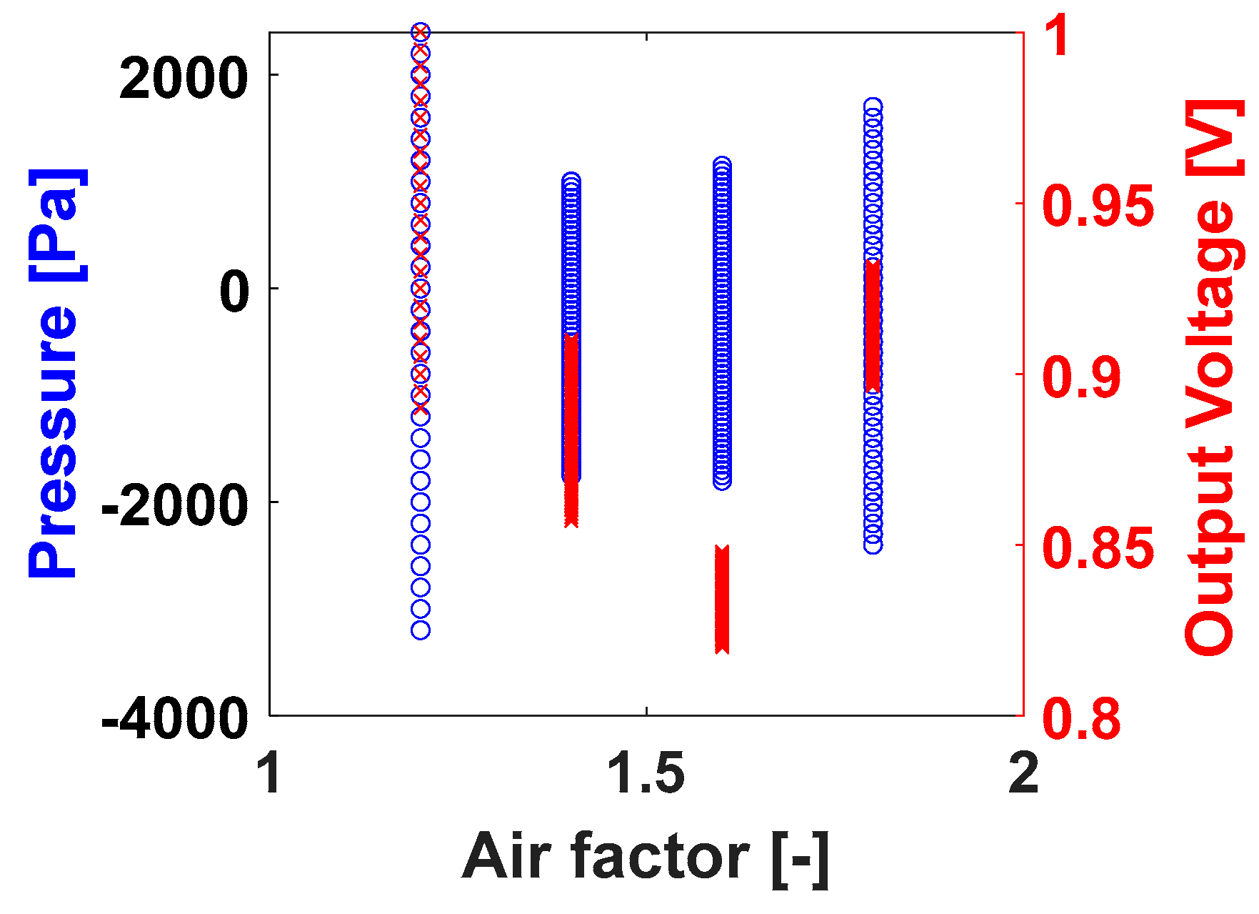
3.4. Bifurcation Diagrams

It was shown above that the combustion system can operate in two stationary modes: one stable low noise level mode and a mode with a fully developed limit cycle oscillation with saturated amplitude. Interesting is the transition between these two modes: what happens in the path from stable to limit cycle, and how does the system return to the stable mode from a limit cycle oscillation? To this end, the traverse between these two modes is explored in both directions. Results of the data obtained from both paths, from stable to unstable and from unstable through 18 different cases, are compared. A preliminary view of this was presented in [17].

The next step to understand how the pressure amplitude distribution changes in the mode transition is by analyzing the bifurcation diagram of the pressure and OH* chemiluminescence values. Figure 11 shows, for the L1 case, the pressure amplitude range (on the left) as a function of decreasing air factor with, on the right, the flame intensity. It is observed that in the stable mode, at high air factor, the range is small, about 400 Pa, and near symmetric around the mean pressure. In the transition the range becomes much larger, around 8000 Pa, and asymmetric with emphasis on the mean pressure. For the case of the PMT signal, the amplitude distribution shows again to be dependent on the air–fuel equivalence factor, and at a lower value of λ, the ranges are much larger than on higher values. Different from the behavior observed with the pressure bifurcation diagram, the values do not concentrate in the middle value of the measured signal, but they are concentrated in the lower values, which makes for a more negatively affected flame intensity by the increasing air.

For the L2 case, Figure 12, the pressure and the intensity signal, where the pressure amplitude range is presented as a function of the decreasing air factor, the ranges do not have a marked tendency when working in learner conditions. The ranges become smaller in the in-between conditions where the system is intermittent. For the case of the intensity, the range of intensity values increases as the air factor decreases, but the values themselves are moving from lower to higher without a clear trend.

4. Nonlinear Analysis

After the relatively simple analysis of the pressure amplitude data, a more mathematical analysis is performed on the basis of the work on strange attractors by Takens [18]. From the obtained time series of the pressure just downstream of the flame, phase space coordinates can be constructed on the basis of the instantaneous values and the value shifted at a certain time delay to generate phase portraits. This system time delay must satisfy the property of being far enough in time that it can be able to generate new data and at the same time close enough to the original so it does not become uncorrelated from it. Takens’ approach to finding this value is through the Average Mutual Information (AMI) function [19], a function that relates two measurements that are close to, but almost independent from, each other by their joint probability density. The appropriate system time delay is then the first minimum when plotting this function with the number of time lags possible.

In this approach, the global embedding dimension is a parameter that must be determined in order to generate the phase space portrait. This parameter gives the lowest integer global dimension, which is the number of dimensions that is necessary to unfold the observed orbits formed by our time series and its delayed copies, and this can be performed by the projection of the attractor to lower-dimensional spaces. A methodology to find this value is through applying the False Nearest Neighbors (FNN) function, which measures the distance between two vectors and finds the nearest neighbor in the phase space. When they are real neighbors, they can go next to the other to form the orbit in the phase portrait. But if they are false, what we see is a projection from a higher dimension, which means that the attractor will not unfold. The dimension that removes all false neighbors and unfolds the attractor is the one defined as the lowest embedding dimension. A more precise explanation of how to determine these two important parameters to obtain the phase space portrait is presented below.

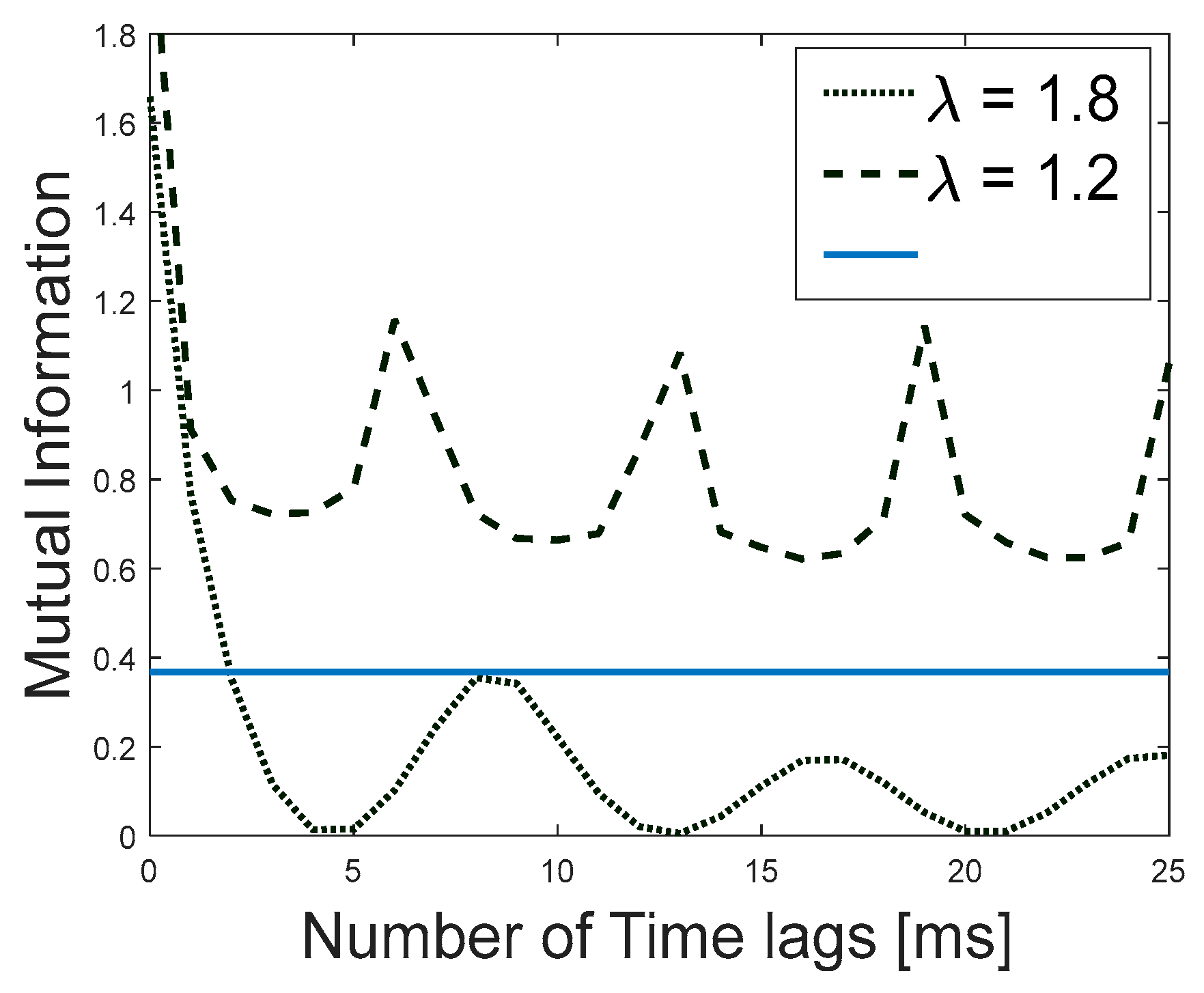
4.1. Average Mutual Information Function

The objective is to create a phase portrait that shows the observed variable (in our case, the pressure), using coordinates made from this same variable and its value further ahead in time at a system characteristic delay time. The system delay time needs to be determined that is far enough in time to generate new data but close enough that it does not become totally independent and uncorrelated. Let us consider a set of measurements $A$ and $B$, with their respective probability densities and joint probability density: $P_A\left(a_i\right)$, $P_B\left(b_j\right)$ and $P_{AB}\left(a_i{b}_j\right)$. The mutual information that gives the interaction between two measurements that are almost independent is then defined as:

$${log}_2\left[{\displaystyle \frac{P_{AB}\left(a_i{b}_j\right)}{{P_A\left(a_i\right)·P}_B\left(b_j\right)}}\right]$$

(1)

When $A$ and $B$ are indeed independent, their mutual information is equal to zero. The Average Mutual Information between both measurements can be defined as:

$$I_{AB}=\sum _{a_i{b}_j}{P}_{AB}\left(a_i{b}_j\right){log}_2\left[{\displaystyle \frac{P_{AB}\left(a_i{b}_j\right)}{P_A\left(a_i\right)P_B\left(b_j\right)}}\right]$$

(2)

As the name suggests, this function gives the relation between these two sets of measurements and their dependence. When adapting to the information from the measurements $s\left(t\right)$ through measurement of $s(t+T),$ the time-lagged measurements, we obtain:

$$I\left(t\right)=s\left(t\right),s\left(t+T\right)P\left(s\left(t\right),s\left(t+T\right)\right){log}_2\left[{\displaystyle \frac{P\left(s\left(t\right),s\left(t+T\right)\right)}{P\left(s\left(t\right)\right)P\left(s\left(t+T\right)\right)}}\right]$$

(3)

The method suggested by Takens is to use the time lag of the first minimum of the Average Mutual Information function as the system time delay.

In Figure 13, we can observe how the AMI data behaves for the two system modes. In both modes, the value of the AMI oscillates as a function of the number of time lags. For the stable mode (left diagram), the AMI value decreases with increasing time lag until eventually the correlation between points in the time series is lost, and the Average Mutual Information function tends to zero. In contrast with this, in the limit cycle oscillation mode the AMI amplitude remains high and constant; the AMI does not vanish with increasing time lag. This means the time series remains correlated in its limit cycle oscillation.

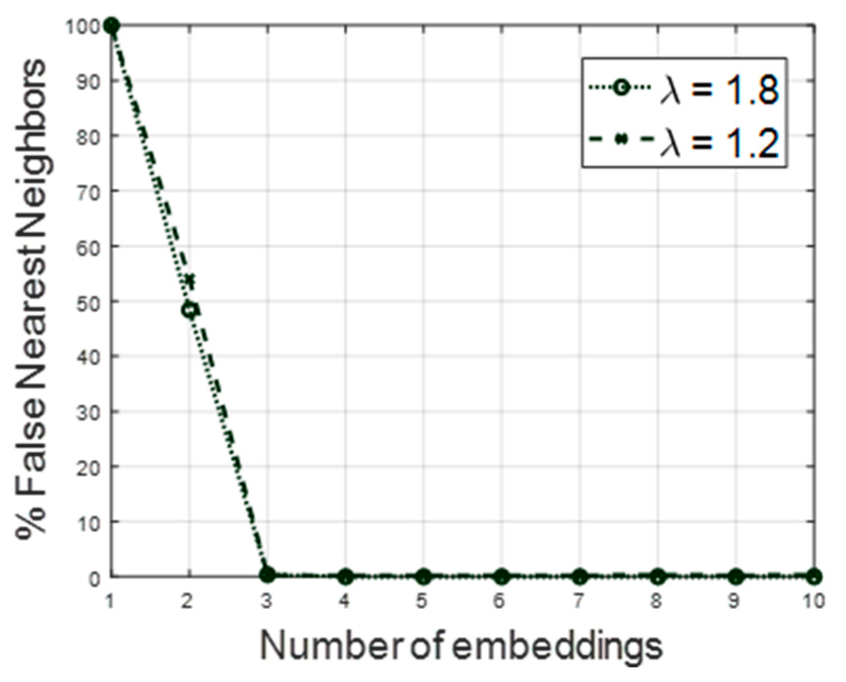
4.2. False Nearest Neighbors Function

To create these phase space reconstructions, we need to determine the integer global dimension, the lowest one, where the necessary number of coordinates to unfold observed orbits from the same signal times the time delay can be performed from the projection of the attractor to a lower-dimensional space. This is known as the embedding dimension. This is a global dimension, and several methods can be found in the literature to find this value. Following Abarbanel’s [14] recommendations and proposed methodology, we can talk about vector neighbors and their neighborhoods and apply this with the False Nearest Neighbors (FNN) function.

We consider two vectors, one of the state space reconstructions in a d dimension:

$$\begin{array}{c}y\left(k\right)=\left[s\left(k\right),s\left(k+T\right),\dots ,(k+\left(d-1\right)T\right]\end{array}$$

(4)

When examining the nearest neighbor in phase space of the vector $y\left(k\right)$ with time label k, we obtain:

$$y^{NN}\left(k\right)=\left[s^{NN}\left(k\right),s^{NN}\left(k+T\right),\dots ,s^{NN}(k+\left(d-1\right)T\right]$$

(5)

The Euclidean distance between these neighbors is:

$$\begin{array}{c}{R}_d{\left(k\right)}^2=m=1d{\left[s\left(k+\left(m-1\right)T\right)s^{NN}(k+\left(m-1\right)T\right]}^2\end{array}$$

(6)

While in dimension $d+1$ is

$$\begin{array}{c}{R}_{d+1}{\left(k\right)}^2=R_d{\left(k\right)}^2+{⌈s\left(k+dT\right)-s^{NN}\left(k+dT\right)⌉}^2\end{array}$$

(7)

If $y\left(k\right)$ is the $y^{NN} \left(k\right)$ neighbor, it can be the one before or next to it but along the orbit, allowing the attractor shape to be identified and compact. If they are false neighbors, this means that the former arrived at the later neighborhood by a projection from a higher dimension and showed that the dimension d does not unfold the attractor. Going to dimension $d+1$, the false neighbor can move out of the neighborhood; we can look for which is the lower dimension that removes all false neighbors and unfold the attractor, and that juncture is known as the $d_E$. Once this point is reached, the addition of dimensions would not change the false neighbor’s percentage.

Through an extended analysis, the criterion established to find two vectors that are false neighbors is that

$${\displaystyle \frac{⌈s\left(k+dT\right)-s^{NN}\left(k+dT\right)⌉}{R_A}}$$

(8)

It is greater than a number of two orders. Considering that R_A is the nominal radius of the attractor defined as the RMS value of the data about its mean.

Figure 14 shows where the percentage of false neighbors drops to zero: 3 for both the air equivalence factor of 1.8 and of 1.2. This means that the phase space reconstruction can be made for the pressure signal in the time lags: $\left[x\right(t),x(t+T{\tau }_s),x(t+2T{\tau }_s\left)\right].$

In Figure 15, we can observe the generated three-phase portraits for a power of 50 kW and the L1, original length. Starting from an air-fuel equivalence ratio, $\lambda =1.8$ and up to 1.2, we can clearly see that for the leaner, stable regime, the three-phase portrait trajectories are all overlapping together, and we cannot distinguish a tendency or a starting point to evaluate our attractors. On the other hand, as on the richer, unstable regime, the attractor unfolds, presenting a torus shape, and the trajectories of the attractor can be noticed. For the case of the PMT signal three-phase portraits, the shapes are not as well defined as the ones provided by the pressure signal, but the trend remains: when moving to stoichiometric combustion, the trajectories unfold towards a torus-like shape.

Figure 16 shows the three-phase portraits under the same condition but for L2, double length. As with previous observations, the formed attractors have interjected trajectories for the stable cases, and for the high-amplitude oscillation case, the attractor unfolds and acquires a torus shape. For the light intensity, the case is similar, but the attractor does not unfold yet in as clear a manner as with the pressure one. Again, when comparing with L1, the high amplitude oscillations are not reached until the $\lambda$ of 1.2.

4.3. Intermittent Case

The obtained three-phase portraits for the intermittent case studied in Section 3.3 are shown in the third row of Figure 16. These plots show that both stable and unstable behavior can be observed: detangled, torus-shaped trajectories tending to higher values and overlapping and jumbled trajectories in the center, crossing values of zero. While in other combustion systems, there is a strong differentiation and even an empty space in between both trajectories tendencies. For this combustor geometry, the three-phase portraits look almost filled, with just a slight separation between the centered trajectories and the torus shape.

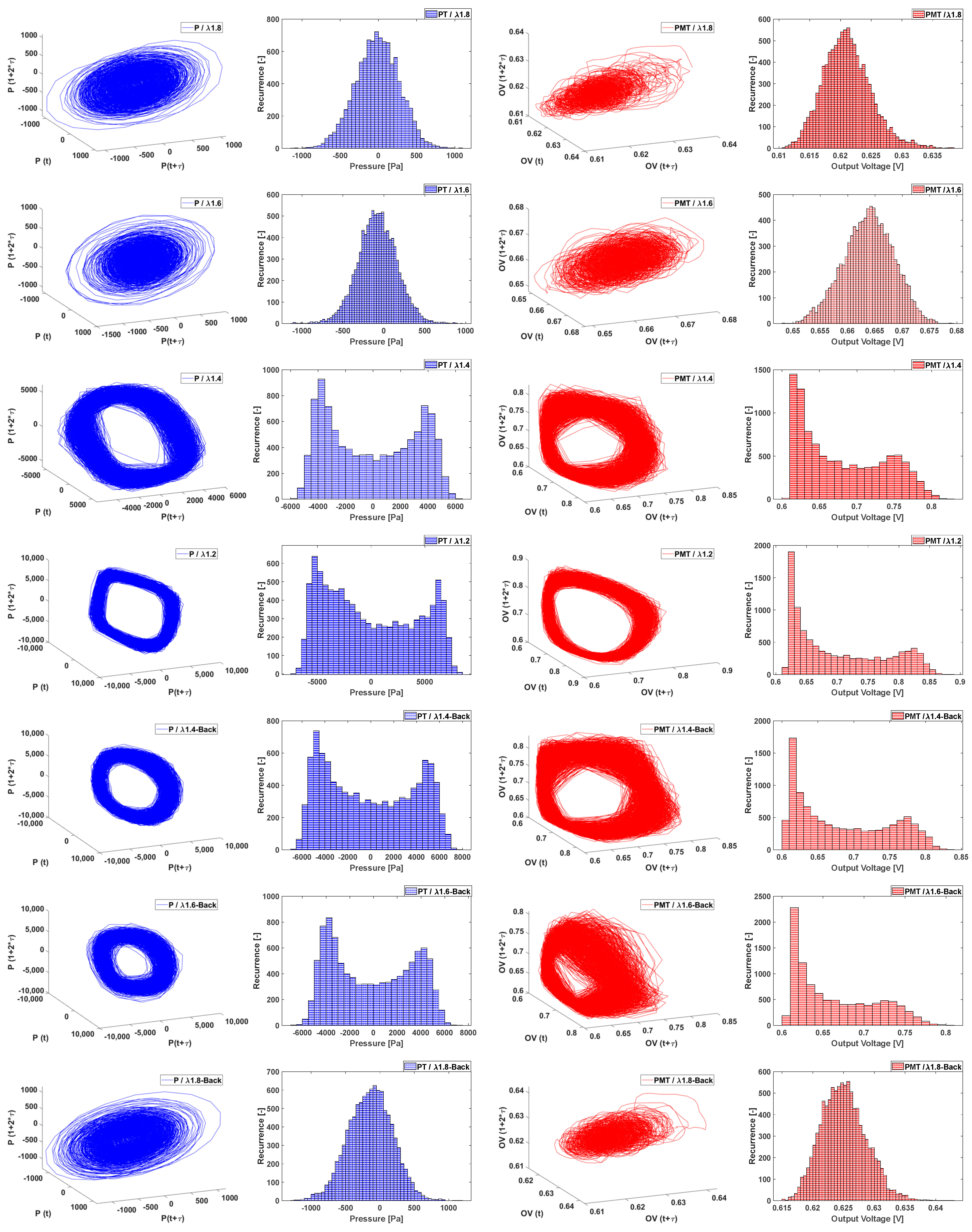
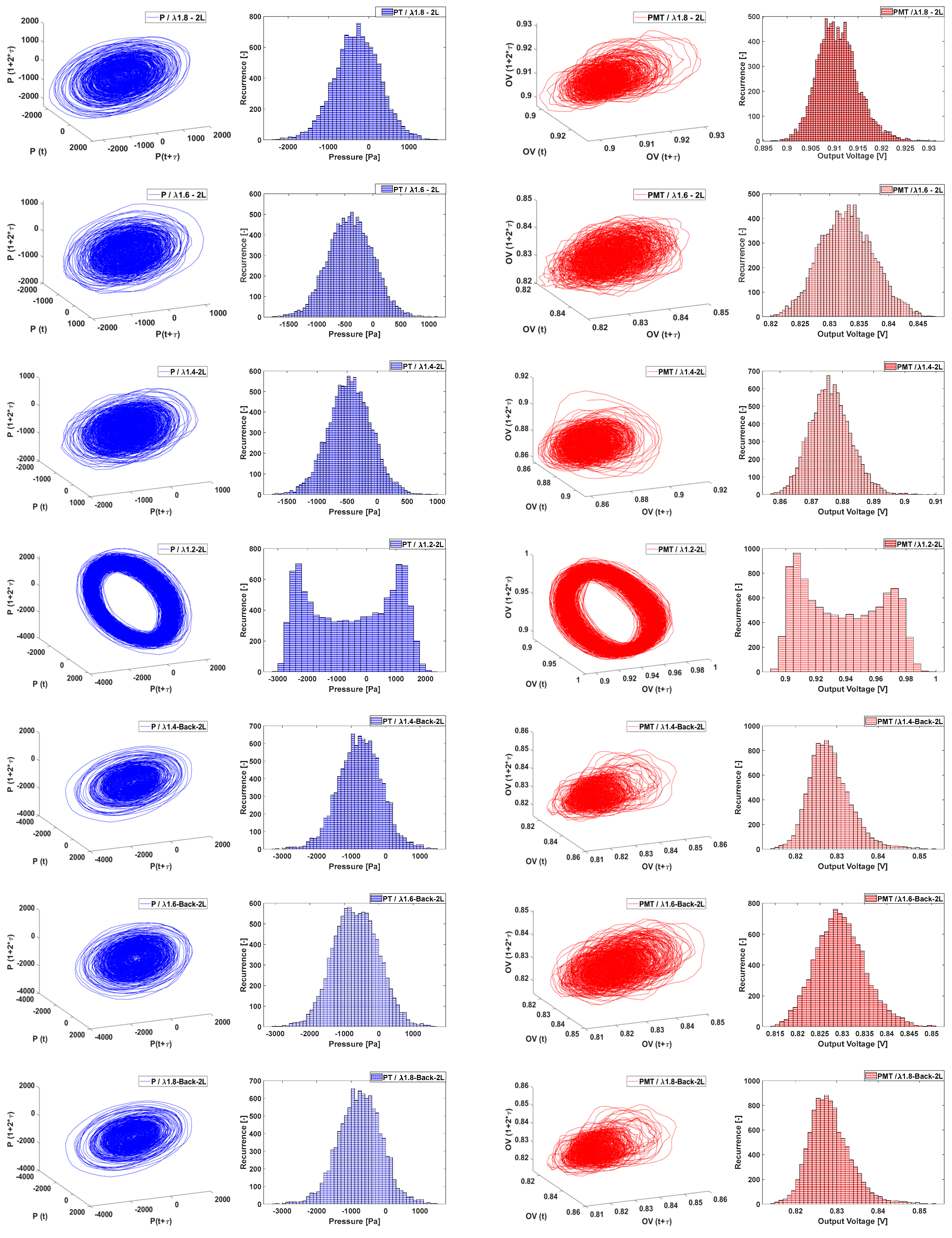
4.4. Hysteresis Effects: Histogram and Phase Portraits Approach

It is known that high-amplitude oscillation has a hysteric effect that can be expressed by means of the Hopf bifurcation point. Hereby, by means of the generated histograms and three-phase portraits of the pressure and flame intensity time series, we can appreciate the resistance of the system to replicate its conditions when these are preceded by certain operating conditions. In Figure 17, we can see that for cases of an air factor from 1.8 to between 1.4 and 1.6 (which implies an increase in fuel mass flow of 14%), in particular coming from a lean (stable) to a richer (unstable case), an intermittent case occurs.

Time series histograms and three-phase portraits, both from the pressure and the flame intensity, going from an air factor of 1.8, the leanest that the combustor allows, to 1.6, 1.4, and 1.2 (the closest to the stoichiometric value that the combustor can stand the elevated temperatures) are shown in Figure 17 and Figure 18. For both, acoustic and flame intensity histogram results reproduce the same behavior. When the air factor is high, there is a bell-shaped distribution that, as we previously acknowledged, has a smaller range. As we decrease the air factor, the bell shape breaks into a bimodal distribution with peaks of similar numbers of data points in its extremes. Finally, in the lowest air factor, the distribution is more irregular, having both a decreasing tendency for half of it and the u-shaped on the other half. Then, when going back in a higher air factor, λ = 1.4, the histogram shape is similar to the previous equal operating condition. Divergent from this case is the following: when going up to λ = 1.6, we still encounter a u-shaped histogram, opposite to the same operating point in the decreasing λ values case, where the histogram was a bell shape. The flame intensity histograms, the ones below and in red, show the same tendency and same resistance to go back in the same shapes for the increasing than for the decreasing of λ, with the notorious difference that the low λ value cases are more of an l-shape histogram than a u-shape. This favors lower values of the intensity rather than higher ones, with a soft peak that then decreases in the highest values.

Regarding the three-phase portrait sequence, we notice that a cleaner, with most trajectories overlapping and making the torus contour thinner, agrees with the operating conditions of the highest amplitude values of the limit cycle oscillations. On the other side of the sequence, the phase portrait has trajectories taking different directions and converging on the center of the plot. As the system becomes more unstable because of less lean conditions, the torus shape is gaining strength, and then, when going back to leaner conditions, the torus shape thickens, and finally all different trajectories converge. For the case of the pressure three-phase portraits, this resistance to “closing the core of the torus shape” is shown at λ = 1.4, where, in the decreasing air-fuel factor case, while open, it is thicker than in the same operating conditions revisited on the increasing sequence. For the case of the flame intensity, these three-phase portraits seem to be affected at all times by the change in conditions, and no plot looks as if it is equivalent on the increasing sequence. As already mentioned, the flame is heavily affected by both turbulence and pressure. The system’s chaotic behavior is complicated and most transparent where these two signals couple for certain frequencies.

From this, we can conclude that the process that holds for this difference between going from the leanest case to a close to stoichiometric versus from the close to stoichiometric to the leanest case is hysteresis induced by nonlinear effects induced by the flow. This is to say that the acoustic and flame intensity behavior is not only a function of the current operating conditions but that they are influenced by the past working state of combustion.

Regarding the differences in behavior related to the geometry, passing from L1 to L2, it can be observed that L2 exhibits greater damping effects. It has been studied [20] that shorter tubes will be less stable because of pressure coupling because of experiments that looked at instabilities for different tube lengths. The length of the tube also affects the transition stages in a very important way. When doubling the length of the liner, we effectively double the volume for the acoustic wave to propagate, which will decrease the amplitude, because the acoustic source and the acoustic energy loss remain constant.

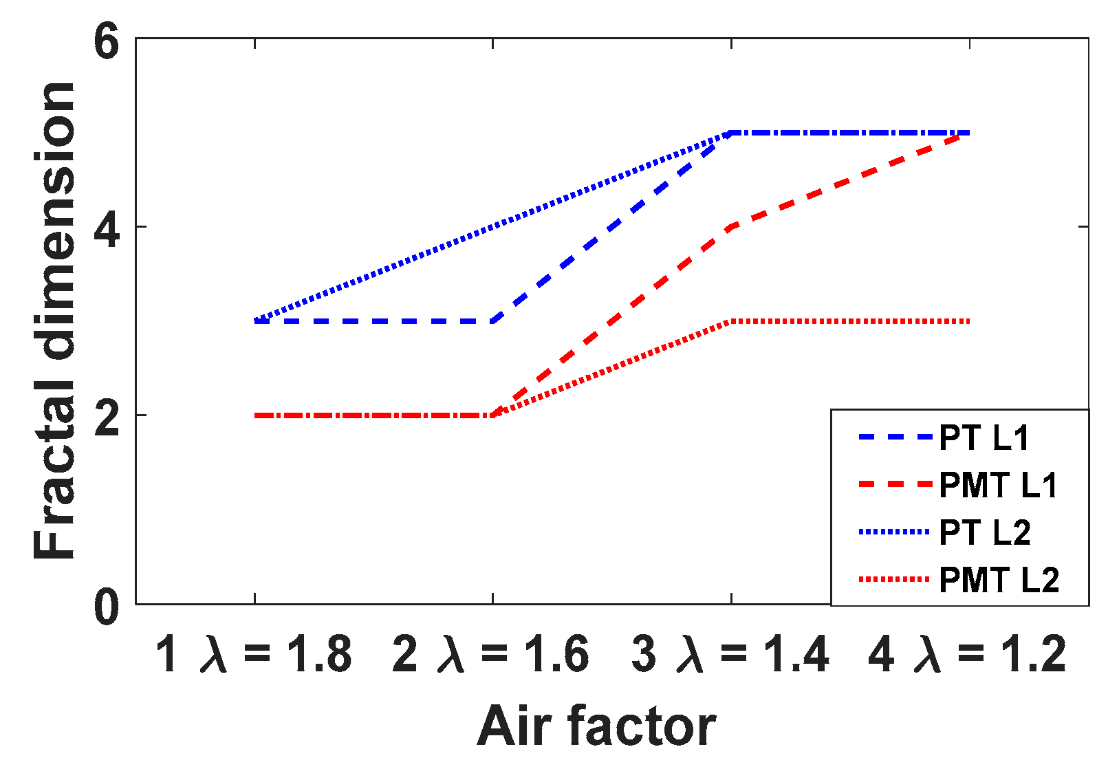
4.5. Fractal Dimension

An important property to characterize the generated attractor in the three-phase portraits that can indicate how to unfold the time series is the fractal dimension. This is a telling quantity that can reveal if a system is likely to show deterministic or chaotic behavior. This fractal dimension must be greater than 2 for a system likely to become chaotic. Several methods are available to find the fractal dimension, accounting for different characteristics for which the original data are available. For the case studied here, we use the “box counting” method, and the results for different operating points for both the standard-length case and the double-length case of the pressure and flame intensity are presented in Figure 19. There is a different behavior for the pressure signal as compared to the signal of the photomultiplier tube (i.e., rate of heat release). It can be observed that at lean air factors (=1.8), the fractal dimensions of both the PT and PMT for both combustor lengths are 2 and 3, respectively. This is the fractal dimension of the system of pressure fluctuations and the chemiluminescence of the flame. The fractal dimension of the flame surface of a premixed flame was studied by Kerstein [21]. There is a strong correlation between the wrinkling of the flame surface and the nature of the flame as a source of sound, as derived by Lighthill. Hence, their fractal dimensions must be correlated as well when the wrinkling is driven by turbulence–combustion interaction. Kerstein predicted a fractal dimension of 7/3 (2.33) for a turbulent premixed flame. This is close to the value for fractal dimensions of 2 and 3 as measured here at air factor 1.8.

This value of the fractal dimension changes when the flame is moving into a limit cycle periodic oscillation due to a coupling of the combustion to the acoustic oscillations. When moving to near stoichiometric combustion (air factor 1.2), the fractal dimension increases to 5 for the PT signal and for the standard length for the PMT signal. For the double length, the fractal dimension increases slightly less to 3 for the PMT signal. This increase in fractal dimension with a decrease in air factor can be explained by the fact that the pressure field and combustion rate fluctuations are driven here by the limit cycle acoustic oscillations. Then, the wrinkling of the flame field is not controlled by combustion–turbulence interaction but by acoustic wave–combustion interaction. Apparently, this leads to an increase in the fractal dimension of the system. Hence, the flame/combustion-acoustic system is developing from marginally chaotic to chaotic when moving from lean to stoichiometric. This is interesting, as in this change in air factor, the combustion-acoustic system develops periodic oscillation with a strange attractor in the phase diagram.

By [22,23], it is suggested that there is a correlation between fractal dimension $D$, flame structure length $l$ and turbulent flame speed $V_f$ given by

$$V_f~l^{D-1}$$

(9)

This equation does raise some questions, as the left- and right-hand sides have different dimensions. They observe for a lean flame a fractal dimension of the flame front of 2 at air factor 1.2, in line with [21]. With the air factor going from lean to stoichiometric, the fractal dimension of the flame is measured by them to decrease to 1.8. With a change to stoichiometric, the turbulent flame speed will increase. Since flame structure length is less than unity, this means the fractal dimension will have to decrease. The difference in behavior with the present work is explained by the fact that the work of [22] is on the wrinkled flame fractal dimension, as determined by turbulence–combustion interaction. The work presented here is dominated by combustion–acoustics interaction at near stoichiometric combustion.

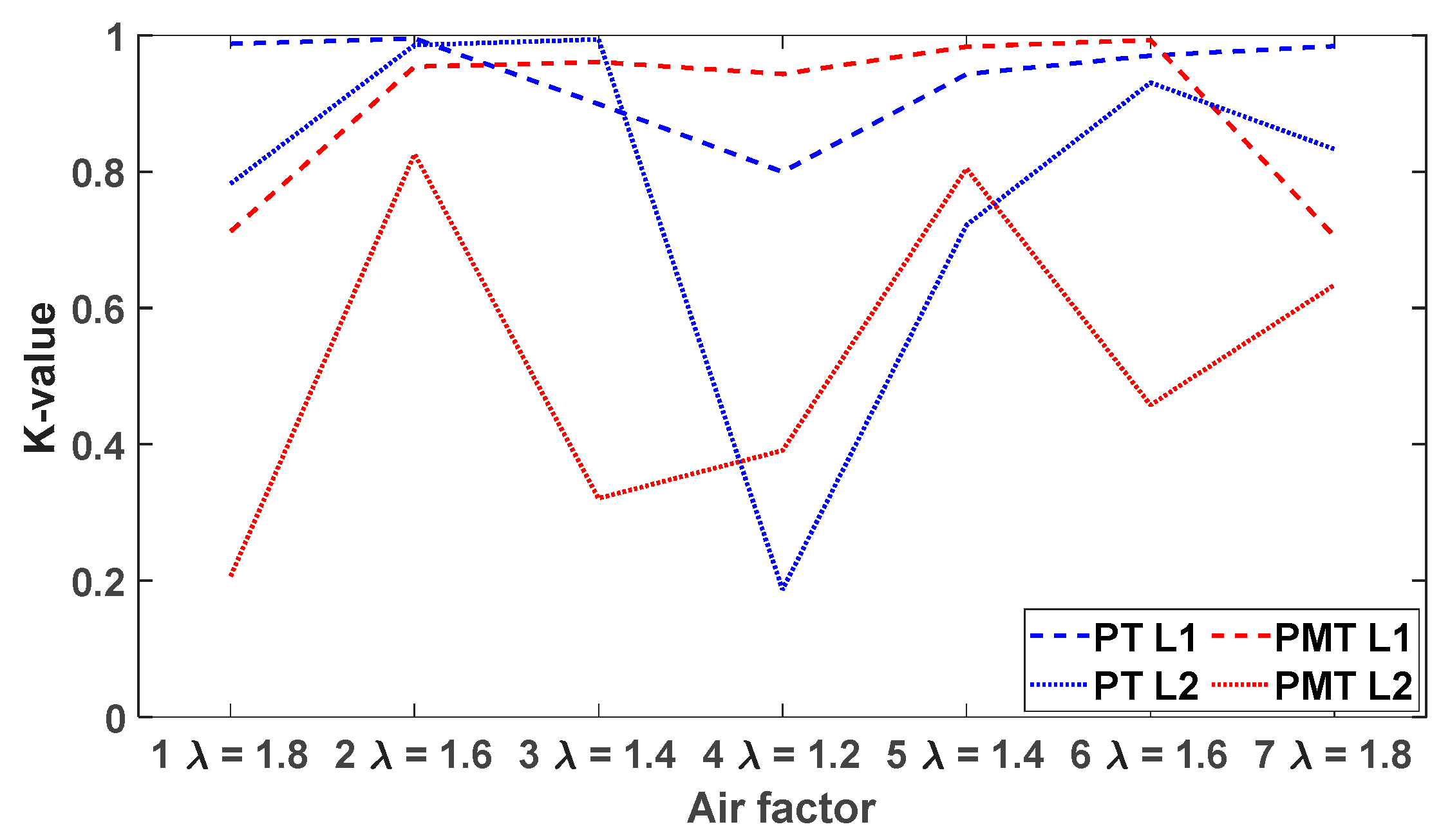
5. The 0-1 Test for Chaos

In the same fashion as [23], when we are presented with the time series and the pressure spectrum of the path from stable to unstable combustion, we do not see just a great change in the amplitude values, but also, we can find some hints in the high amplitude cases of the presence of deterministic non-chaotic behavior.

There are several techniques to evaluate the presence of chaos in a system; for this study, we decided on the 0-1 test, as first proposed by Gottwald and Melbourne [24]. This is under the notion that the methodology is very adaptable to a system of our kind and because the results have a visual appeal to our path kind of study.

This method was proposed as an alternative to the Lyapunov exponent for determining if a system is chaotic or not while offering the advantage of treating the data regardless of its dimension. It uses a time series as input data, and the output can be 0, related to a non-chaotic system, or 1, for a chaotic one.

For a given series, being these $\varphi \left(j\right)$ with $j=1,\dots N$, we obtain the translation variables, which are as follows:

$$p_c\left(n\right)={\sum }_{j=1}^n\varphi \left(j\right)\mathit{cos}\left(jc\right)$$

(10)

$$q_c\left(n\right)={\sum }_{j=1}^n\varphi \left(j\right)\mathit{sin}\left(jc\right)$$

(11)

For $n=\mathrm{1,2},\dots N$. Here, the diffusive or not diffusive behavior of $p_c$ and $q_c$ can be investigated by analyzing the mean square displacement $M_c\left(n\right).$ This test shows that if the dynamics of the given system have a regular behavior, then the mean square displacement will be bounded as a function of time. On the other hand, if the studied system is chaotic, it will scale linearly with time. From this we can assure that we have a mean square displacement that is a function of time, as shown in Equation (3).

$$M_c\left(t\right)=\underset{T\to \infty }{\mathit{lim}}{\int }_0^T{\left(p_c\left(t+\tau \right)-p_c\left(\tau \right)\right)}^2+{\left(q_c\left(t+\tau \right)-q_c\left(\tau \right)\right)}^{2}dt$$

(12)

And from this, we can obtain an approximation that accounts for a sample time ${\tau }_s$ to Equation (4).

$$M_c\left(n\right)=\underset{T\to \infty }{\mathit{lim}}{\int }_0^T{\left(p_{c{\tau }_s}\left(j+n\right)-p_{c{\tau }_s}\left(j\right)\right)}^2+{\left(q_{c{\tau }_s}\left(j+n\right)-q_{c{\tau }_s}\left(j\right)\right)}^{2}d\tau$$

(13)

For the case of continuous time systems, the mean square displacement is defined as:

$$D_c\left(n\right)=M_c\left(n\right)-V_{osc}\left(c.n\right)$$

(14)

where $V_{osc}(c.n)$ accounts for an oscillatory term that is obtained from

$$V_{osc}\left(c.n\right)={\left(E\varphi \right)}^2{\displaystyle \frac{1-cos\left(nc\right)}{1-cos\left(c\right)}}$$

(15)

We want to find and express the asymptotic growth rate, $K_c$, and if the value is closer to 0, it means that our data are deterministic (non-chaotic or limit cycle oscillations), or if it is closer to 1, it means that our data are chaotic. In order to obtain these values, we use the regression method. This method consists of having a linear regression for the log-log plot for the $M_c \left(n\right),$ so we have Equation (16):

$$K_c=\underset{n\to \infty }{\mathit{lim}}{\displaystyle \frac{log{M}_c\left(n\right)}{\mathit{log}n}}$$

(16)

The data obtained from the experiments are implemented for this test. The transition from stable state to unstable and then from unstable to stable is analyzed for both the pressure and the OH* chemiluminescence signals and for cases L1 and L2, as can be seen in Figure 20. When plotting the K values for both the pressure (in black) and the PMT signal (in red), we can see that when going from right to left at high λ values, K has values for pressure close to unity, confirming the presence of chaos and an absence of a periodic limit cycle, in line with the absence of low-dimensional attractors in the three-phase portraits. Then, at λ = 1.2, the value decays to a minimum. This indicates the transition to a low-dimensional strange attractor due to a deterministic periodic limit cycle oscillation. When moving further to the left to higher air factors, the value of K goes back up again, but with lower values than in the decreasing sequence but close enough to unity (higher than 0.6). This confirms the earlier observations of hysteresis and the reluctance of the system to leave the deterministic oscillation once this has formed.

The behavior of the PMT signal (rate of heat release) is more complicated, and the data are less straightforward. When at a high air factor, the K value is small and indicates deterministic behavior, which is in contradiction with the observed three-phase portraits. At intermediate air factor 1.6, the K value increases to unity, confirming chaotic behavior. At the minimum air factor, the K value decreases again to zero, indicating deterministic behavior. It can be concluded that at an intermediate to stoichiometric air factor, the K value for the PMT signal is a good measure for deterministic behavior, but in lean conditions, this is not the case. For the double length, the K variation is more extreme, possibly due to the large damping in the system.

In addition to this test, the Lyapunov exponent for confirmation of chaotic behavior is presented in Figure 21, obtained from the calculation method proposed by [25]. The Lyapunov exponent is a measure of the rate of separation of nearby trajectories in a dynamical system, which allows one to perceive the chaotic nature of a system. When comparing it with Figure 20, we can appreciate a similar behavior for predicting the onset of chaos and instability.

6. Conclusions

In this experimental study, the chaotic nature of the pressure and combustion rate oscillations of a premixed atmospheric combustor was studied as a function of air factor and combustor length. There is a significant difference in the behavior of the combustor at standard length and double length. At both lengths the combustion is stable and dominated by combustion–turbulence interaction at lean conditions. Near stoichiometric, the combustion reaches a limit cycle oscillation driven by acoustics–combustion interaction. The combustion dynamics differ, and the operating condition to reach the limit cycle oscillations moves in the sense that a smaller combustor length reaches the instability with leaner conditions. In addition to this, a longer liner length allows for an intermittent state where both stable and unstable modes coexist. Related to the instability frequencies presented for both cases, for the standard-length case, high amplitude oscillations occur at 246.4 Hz, 492.9 Hz, and 740.8 Hz, whereas for the double-length case, the high amplitude oscillations are located at 165.5 Hz, 331.9 Hz, and 656.9 Hz. The three-phase diagram generated for the pressure and chemiluminescence fluctuations develops from a chaotic diagram to a diagram with a strange attractor when moving from lean to rich combustion and into a limit cycle operation. In this change the amplitude distribution changes from a Gaussian shape to a flat distribution up to the maximum amplitude. For both length cases of high-amplitude oscillations, a hysteresis effect is observed when it is moved towards unstable cases and out of them. Subsequently, the fractal dimension of the pressure and chemiluminescence fluctuations was determined. At lean combustion, where the combustion is coupled primarily to turbulence, the fractal dimension of pressure is 2 and chemiluminescence is 3, in line with predictions by literature. When close to stoichiometric, the fractal dimension increases to 5 due to a switch to combustion fluctuations dominated by acoustics. Finally, a 0-1 test was performed to investigate if this can indicate an imminent change from stable to unstable combustion. This is confirmed with a change in the value of $K$ from unity to a low value when the unstable operation near stoichiometric is approached. The final conclusion is that postprocessing of measured pressure fluctuations or chemiluminescence is a powerful tool to analyze, characterize, and predict the behavior of a confined flame in a combustor. Of particular interest is the development of methods like the 0-1 test and the fractal dimension calculation so they can be measured in real time so this can be used as a warning that the gas turbine is reaching limit cycle conditions on time for a change in the operating parameters to stop the limit cycle on time and avoid damaging the gas turbine.

References

1. Ourbak, T.; Tubiana, L. Changing the game: The Paris Agreement and the role of scientific communities. Clim. Policy 2017, 17, 819–824. [Google Scholar] [CrossRef]
2. Pashchenko, D. Hydrogen-rich gas as a fuel for the gas turbines: A pathway to lower CO2 emission. Renew. Sustain. Energy Rev. 2023, 173, 113117. [Google Scholar] [CrossRef]
3. Poinsot, T. Prediction and control of combustion instabilities in real engines. Proc. Combust. Inst. 2017, 36, 1–28. [Google Scholar] [CrossRef]
4. Zhao, D.; Lu, Z.; Zhao, H.; Li, X.Y.; Wang, B.; Liu, P. A review of active control approaches in stabilizing combustion systems in aerospace industry. Prog. Aerosp. Sci. 2018, 97, 35–60. [Google Scholar] [CrossRef]
5. Gotoda, H.; Nikimoto, H.; Miyano, T.; Tachibana, S. Dynamic properties of combustion instability in a lean premixed gas-turbine combustor. Chaos 2011, 21, 013124. [Google Scholar] [CrossRef]
6. Kabiraj, L.; Sujith, R.I.; Wahi, P. Bifurcations of self-excited ducted laminar premixed flames. J. Eng. Gas Turbines Power 2012, 134, 031502. [Google Scholar] [CrossRef]
7. Roy, A.; Premchand, C.P.; Raghunathan, M.; Krishnan, A.; Nair, V.; Sujith, R.I. Critical region in the spatiotemporal dynamics of a turbulent thermoacoustic system and smart passive control. Combust. Flame 2021, 226, 274–284. [Google Scholar] [CrossRef]
8. Nair, V.; Sujith, R.I. Multifractality in combustion noise: Predicting an impending combustion instability. J. Fluid Mech. 2014, 747, 635–655. [Google Scholar] [CrossRef]
9. Unni, V.R.; Yogesh Prasaad, M.S.; Ravi, N.T.; Iqbal, S.M.; Pesala, B.; Sujith, R.I. Experimental investigation of bifurcations in a thermoacoustic engine. Int. J. Spray Combust. Dyn. 2015, 7, 113–130. [Google Scholar] [CrossRef]
10. Karlis, E.; Liu, Y.; Hardalupas, Y.; Taylor, A.M.K.P. H2 enrichment of CH4 blends in lean premixed gas turbine combustion: An experimental study on effects on flame shape and thermoacoustic oscillation dynamics. Fuel 2019, 254, 115524. [Google Scholar] [CrossRef]
11. Palies, P.; Durox, D.; Schuller, T.; Candel, S. Nonlinear combustion instability analysis based on the flame describing function applied to turbulent premixed swirling flames. Combust. Flame 2011, 158, 1980–1991. [Google Scholar] [CrossRef]
12. Zhang, B.; Shahsavari, M.; Rao, Z.; Yang, S.; Wang, B. Thermoacoustic instability drivers and mode transitions in a lean premixed methane-air combustor at various swirl intensities. Proc. Combust. Inst. 2021, 38, 6115–6124. [Google Scholar] [CrossRef]
13. Bakker, R.; Schouten, J.C.; Giles, C.L.; Takens, F.; Bleek, C.M. van den Learning Chaotic Attractors by Neural Networks. Neural Comput. 2000, 12, 2355–2383. [Google Scholar] [CrossRef]
14. Farmer, J.D.; Sidorowich, J.J. Predicting chaotic time series. Phys. Rev. Lett. 1987, 59, 845–848. [Google Scholar] [CrossRef] [PubMed]
15. Abarbanel, H.D.I. Analysis of Observed Chaotic Data; Springer: New York, NY, USA, 1996; ISBN 978-0-387-98372-1. [Google Scholar]
16. Kobayashi, T.; Murayama, S.; Hachijo, T.; Gotoda, H. Early Detection of Thermoacoustic Combustion Instability Using a Methodology Combining Complex Networks and Machine Learning. Phys. Rev. Appl. 2019, 11, 1. [Google Scholar] [CrossRef]
17. Arredondo, S.N.; Kok, J. A model to study spontaneous oscillations in a lean premixed combustor using non linear analysis. In Proceedings of the 26th International Congress on Sound and Vibration, ICSV 2019—Hotel Bonaventure, Montreal, QC, Canada, 7–11 July 2019; pp. 1–8. [Google Scholar]
18. Takens, F. Detecting Strange Attractors in Turbulence; Springer: Berlin/Heidelberg, Germany, 1981; pp. 366–381. [Google Scholar]
19. Wallot, S.; Mønster, D. Calculation of Average Mutual Information (AMI) and false-nearest neighbors (FNN) for the estimation of embedding parameters of multidimensional time series in matlab. Front. Psychol. 2018, 9, 1679. [Google Scholar] [CrossRef] [PubMed]
20. Dubey, A.K.; Koyama, Y.; Hashimoto, N.; Fujita, O. Effect of geometrical parameters on thermo-acoustic instability of downward propagating flames in tubes. Proc. Combust. Inst. 2019, 37, 1869–1877. [Google Scholar] [CrossRef]
21. KERSTEIN, A.R. Fractal Dimension of Turbulent Premixed Flames. Combust. Sci. Technol. 1988, 60, 441–445. [Google Scholar] [CrossRef]
22. Noguchi, Y.; Nakamura, K.; Hagiwara, Y.; Hitomi, S.; Kuwana, K. Flame Propagation and Fractal Dimension in a Concentric Double Cylinders Apparatus. J. Jpn. Soc. Exp. Mech. 2014, 14, s101–s104. [Google Scholar] [CrossRef]
23. Guan, Y.; Gupta, V.; Li, L.K.B. Intermittency route to self-excited chaotic thermoacoustic oscillations. J. Fluid Mech. 2020, 894, R3. [Google Scholar] [CrossRef]
24. Gottwald, G.A.; Melbourne, I. A new test for chaos in deterministic systems. Proc. R. Soc. A Math. Phys. Eng. Sci. 2004, 460, 603–611. [Google Scholar] [CrossRef]
25. Rosenstein, M.T.; Collins, J.J.; De Luca, C.J. A practical method for calculating largest Lyapunov exponents from small data sets. Phys. D Nonlinear Phenom. 1993, 65, 117–134. [Google Scholar] [CrossRef]
Figure 1. LIMOUSINE combustor layout.
Energies 18 01852 g001
Figure 2. The triangular wedge flame holder and its mounted position in the combustor.
Energies 18 01852 g002
Figure 3. Snapshot of the flame from the side of the combustor. Air factors of 1.8 (left) and 1.2 (right).
Energies 18 01852 g003
Figure 4. Acoustic in units of gauge pressure (blue) and PMT/heat release in units of output voltage (red) for a λ of 1.8. Power spectra (top), histograms (middle), and time series (bottom).
Energies 18 01852 g004
Figure 5. Acoustic in units of gauge pressure (blue) and PMT/heat release in units of output voltage (red) for λ of 1.2. Power spectra (top), histograms (middle), and time series (bottom).
Energies 18 01852 g005
Figure 6. Cross spectrum of the oscillation of gauge pressure and PMT/heat release output voltage for magnitude (top), phase (middle), and coherence (bottom). Results are shown for air factors 1.8, 1.6, 1.4, and 1.2 with the standard combustor length.
Energies 18 01852 g006
Figure 7. Acoustic in units of gauge pressure (blue) and PMT/heat release in units of output voltage (red) for λ of 1.8. Power spectra (top), histograms (middle), and time series (bottom). Double length.
Energies 18 01852 g007
Figure 8. Acoustic in units of gauge pressure (blue) and PMT/heat release in units of output voltage (red) for λ of 1.2. Power spectra (top), histograms (middle), and time series (bottom). Double length.
Energies 18 01852 g008
Figure 9. Cross spectrum of the oscillation of gauge pressure and PMT/heat release output voltage for magnitude (top), phase (middle), and coherence (bottom). Results are shown for air factors 1.8, 1.6, 1.4, and 1.2 with double combustor length.
Energies 18 01852 g009
Figure 10. Acoustic in units of gauge pressure (blue) and PMT/heat release in units of output voltage (red) for λ of 1.6. Power spectra (top), histograms (middle), and time series (bottom). Double length.
Energies 18 01852 g010
Figure 11. Bifurcation diagram for standard length (L1) for the acoustics/pressure (blue o) and rate of heat release/PMT output voltage (red x) signals.
Energies 18 01852 g011
Figure 12. Bifurcation diagram for double length (L2) for the acoustics/pressure (blue o) and heat release/PMT output voltage (red x) signals.
Energies 18 01852 g012
Figure 13. AMI function for an air–fuel equivalence factor of 1.8 (dot) and for one of 1.2 (dashed).
Energies 18 01852 g013
Figure 14. Percentage of False Nearest Neighbors for an air factor of 1.8 (dot) and for one of 1.2 (dashed).
Energies 18 01852 g014
Figure 15. Three-phase portraits for L1. Gauge pressure (P) in blue and PMT/heat release (output voltage, OV) in red for λ 1.8, 1.6, 1.4, and 1.2.
Energies 18 01852 g015
Figure 16. Three-phase portraits for L2. Gauge pressure (P) in blue and PMT/heat release (output voltage, OV) in red for λ 1.8, 1.6, 1.4, and 1.2.
Energies 18 01852 g016
Figure 17. Three-phase portraits and histograms for gauge pressure in blue and PMT/heat release for L1, following the sequence λ 1.8 (top), 1.6, 1.4, 1.2, 1.4, 1.6, and 1.8 (bottom).
Energies 18 01852 g017
Figure 18. Three-phase portraits and histograms for gauge pressure in blue and PMT/heat release for L2, following the sequence λ 1.8 (top), 1.6, 1.4, 1.2, 1.4, 1.6, and 1.8 (bottom).
Energies 18 01852 g018
Figure 19. Fractal dimension for both L1 (- -) and L2 (…), for gauge pressure (blue) and PMT/heat release (red).
Energies 18 01852 g019
Figure 20. The 0-1 test for chaotic behavior for both L1 (- -) and L2 (…), for gauge pressure (blue) and PMT/heat release (red).
Energies 18 01852 g020
Figure 21. Lyapunov exponent for both L1 (- -) and L2 (…), for gauge pressure (blue) and PMT/heat release (red).
Energies 18 01852 g021
Disclaimer/Publisher’s Note: The statements, opinions and data contained in all publications are solely those of the individual author(s) and contributor(s) and not of MDPI and/or the editor(s). MDPI and/or the editor(s) disclaim responsibility for any injury to people or property resulting from any ideas, methods, instructions or products referred to in the content.