Optimal Economic Dispatch Strategy for Cascade Hydropower Stations Considering Electric Energy and Peak Regulation Markets

Abstract

With the evolution of the power market and the increase in the new energy penetration rate, the power industry will present diversified characteristics. The continuous development of the electric energy market (EEM) and the peak regulation market (PRM) is also affecting the economic benefits of cascade hydropower stations, in which the EEM, as a market for electric energy trading in the power market, develops synergistically with the PRM and creates the conditions for the consumption of new energy sources; for this reason, this paper, while considering the benefits of cascade hydropower stations in the EEM in different time scales and the impact of the spot market, combines the compensation mechanism and apportionment principle of the PRM. This paper proposes an optimal economic scheduling strategy for cascade hydropower stations. Specifically, firstly, the strategy adopts multi-objective optimization. The objective function takes into account the generation capacity of the cascade hydropower stations, the benefits of the EEM, the influence of the spot market, the compensatory benefits of peaking, and the sharing expenses of peaking; secondly, the constraints at the level of the power grid, the level of the cascade hydropower stations, and the level of the market are taken into account comprehensively, and the Harris Hawk Algorithm is used to solve the model; lastly, by comparing different schemes, it is observed that under varying inflow conditions, the proposed dispatch strategy in this paper yields slightly lower revenue in the EEM than other schemes. However, due to its comprehensive consideration of the synergy between the PRM and the EEM, its overall economic benefits surpass those of other schemes. This fully validates the effectiveness and economic efficiency of the proposed dispatch strategy.

1. Introduction

Given the increasingly serious global energy crisis and environmental pollution, energy saving and emission reduction in the power industry have received great attention. The development and utilization of clean energy such as wind and hydropower have become a hot research topic under the background of the national strategies of ‘Carbon Peak, Carbon Neutral’ [1] and the construction of a new type of electric power system with new energy as the main body. Wind power and photovoltaic power generation are extremely dependent on natural conditions, and the instability of wind speed and sunshine leads to large fluctuations in power generation, making it difficult to ensure continuous and stable power output [2]. This intermittency means that wind and solar power cannot provide a constant and reliable supply of electricity, so there is an urgent need to strengthen the construction of the peak capacity of the power system [3].

With strong anti-disturbance regulation capability and flexible operation, cascade hydropower stations are an ideal regulating power source [4]. Along with the process of power market reform, cascade hydropower stations with regulating capability can effectively suppress the volatility of wind power [5]; however, due to the continuous improvements in the mechanisms of the EEM [6] and PRM, the benefits of cascade hydropower stations will be affected by new energy sources such as wind power; therefore, it is necessary to clarify how to maximize the benefits of cascade hydropower stations in participating in the EEM and PRM [7]. Therefore, there is an urgent need to clarify how to maximize the efficiency of the cascade hydropower stations in participating in the EEM and PRM. Therefore, this paper proposes a scheduling strategy for cascade hydropower stations under the consideration of the EEM and PRM from the point of view of the benefits of the cascade hydropower stations themselves [8].

Currently, there is limited research, both domestically and internationally, that incorporates the EEM and PRM into the economic dispatch operation of cascade hydropower stations. In many countries and provinces, these markets are still in the experimental stage [9], and the boundaries set by the operating experience of the electricity market are difficult to adapt to the stochastic fluctuations of new energy sources and load variations. This makes it challenging to accurately characterize system dynamics, thereby increasing the difficulty of precise economic dispatch for cascade hydropower stations in the current context. Reference [10] proposed an optimal trading strategy for hydropower stations participating in the EEM based on sequential clearing using distributional regression. Tian et al. [11] conducted a study on the operation of hydropower stations within the EEM environment and developed an optimization model for market declaration. In the literature [12], a stochastic optimization model was formulated for the participation of cascade hydropower stations in the day-ahead market and the secondary frequency regulation market, resulting in an operation plan that maximizes expected profits in both the electric energy and frequency regulation markets simultaneously. Authors [13] introduced a price-risk-based scheduling model for cascade hydropower stations participating in the EEM, which was applied to the day-ahead market declaration. The literature [14] focuses on maximizing revenue in the EEM, considering unit efficiency and head constraints, and employing a dynamic planning model to address the short-term scheduling problem of hydropower stations. The literature [15] examines the scheduling problem of cascade hydropower stations and pumped-storage stations participating in both the EEM and the spinning reserve market. Men et al. [16] use the Kamchay and Lower Sesan hydropower stations as case studies, providing a detailed analysis of the benefit compensation mechanisms under various ancillary markets in hydropower projects.

However, scholars, both domestically and internationally, have employed a variety of methods to address the optimization scheduling problem of cascade hydropower stations. Yuan et al. [17] considered both power generation and ecological protection objectives, and a comprehensive decision-making model for the optimal operation of cascade hydropower stations was developed, with the NSGA-II algorithm used to solve the optimization framework. In reference [18], an enhanced lightning search algorithm was applied to solve the scheduling model of cascade hydropower stations, with a particular emphasis on the stations’ internal constraints, resulting in improved solution accuracy. Zhu et al. [19] proposed a new clearing method for the cascade hydropower spot market. Introducing the water–electricity coupling degree (WCD) index and a multi-objective optimization model effectively alleviates the contradiction between water wastage and water shortage in hydropower stations after market clearing. Lu et al. [20] proposed a risk measurement method based on the Conditional Value at Risk (CVaR) to quantify the risk of renewable energy generation on the revenue of an energy portfolio. The superiority of the proposed approach is demonstrated by comparing it with methods that only consider spot price fluctuations. In reference [21], an energy allocation method for adjustable hydropower plants based on a time-varying relative risk aversion coefficient (TVRRA) is proposed. The method uses a two-layer optimization model to adjust the energy distribution of the hydropower plant, making it more aligned with practical decision-making needs.

Domestic and international scholars have made notable contributions to the research on cascade hydropower station participation in the electricity market. However, several gaps remain.

Firstly, most studies focus on the spot market, with limited research on the combined effects of the PRM and EEM on cascade hydropower stations.

Secondly, while many studies on the EEM examine the profits of cascade hydropower stations in the spot market, few address the negative impacts of new-energy participation in the spot market on these stations.

Lastly, in the field of ancillary services, there is a lack of research that separately examines the compensatory benefits and cost-sharing aspects of cascade hydropower stations’ participation in the PRM.

Given the existing research gaps in cascade hydropower stations, developing a dispatch strategy that integrates both the EEM and PRM is especially important. The specific approach in this study is as follows:

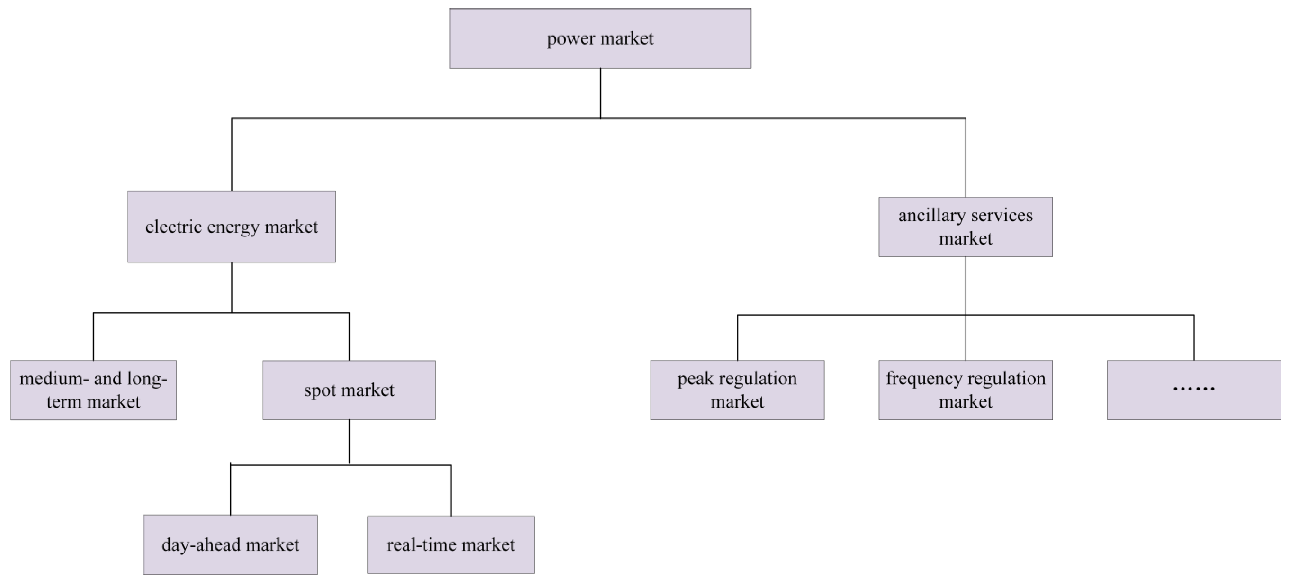
• Introduction to the power market framework

This paper first presents the fundamental framework of the power market, detailing the coupled mathematical models of various market levels within the EEM. Additionally, it introduces the compensation mechanism and cost-sharing principles of the PRM, providing the theoretical foundation for the objective function proposed later.

2.

Formulation of the objective function

The objective function is developed by comprehensively considering multiple factors, including power generation, economic benefits in the EEM, the impact of the spot market, peak regulation compensation, and cost-sharing expenses. The Analytic Hierarchy Process (AHP) is employed to determine the weights of the objective function components. Furthermore, by incorporating constraints at the grid level, hydropower station level, and market level, a mathematical model for the dispatch of cascade hydropower stations is established.

3.

Determine the solution method

To efficiently solve the multi-objective optimization problem, the Harris Hawks Optimization (HHO) algorithm is adopted, given its capability to rapidly converge to the global optimum. This approach ensures the effective and robust optimization of the proposed dispatch strategy.

4.

Conduct simulation verification

Finally, since the output of cascade hydropower stations depends on inflow conditions, two scenarios—high flow (wet season) and low flow (dry season)—are established based on actual dispatching rules. Scheduling schemes for cascade hydropower stations under these different conditions are obtained, and control schemes are designed for each scenario. The results demonstrate the effectiveness and economic feasibility of the proposed scheduling strategy.

The innovation of this study accounts for both the positive benefits and potential negative impacts of the dispatch strategy under the EEM and PRM. Specifically, in the EEM, the model considers power generation, revenue obtained from market participation across different time scales, and the negative impact of electricity price fluctuations caused by the uncertainty of new energy output in the spot market. In the auxiliary market, the model incorporates the compensation earned by cascade hydropower stations in deep peaking and the cost-sharing when thermal power units participate in deep peaking. In conclusion, as the power market continues to evolve and the penetration of renewable energy increases, this strategy highlights how cascade hydropower stations can optimize their economic benefits amid a complex and dynamic external environment. The findings offer valuable insights for the future dispatch optimization of cascade hydropower stations.

2. Theoretical Analysis of Cascade Hydropower Stations’ Participation in the EEM and PRM

As shown in Figure 1, with the ongoing development of the domestic power market, it is primarily divided into two main sectors: the electric energy market and the ancillary services market.

The EEM is responsible for trading electricity commodities within the power market system. From a temporal perspective, it can be categorized into medium- and long-term markets and spot markets, with the latter further subdivided into day-ahead and real-time markets. Medium- and long-term transactions offer market participants stability and predictability, while spot trading provides mechanisms for price discovery and flexible adjustments.

The ancillary services market primarily encompasses the PRM, frequency regulation market, and so on due to the ongoing development and updates in the ancillary services market, and the significant impact of the PRM and frequency regulation markets on cascade hydropower stations. Therefore, certain ancillary markets are omitted in this study. While considerable research has been conducted on aspects such as frequency regulation, studies focusing on the PRM remain relatively scarce. Therefore, this study concentrates on the impact of the PRM within the ancillary services sector on the scheduling of cascade hydropower stations [22].

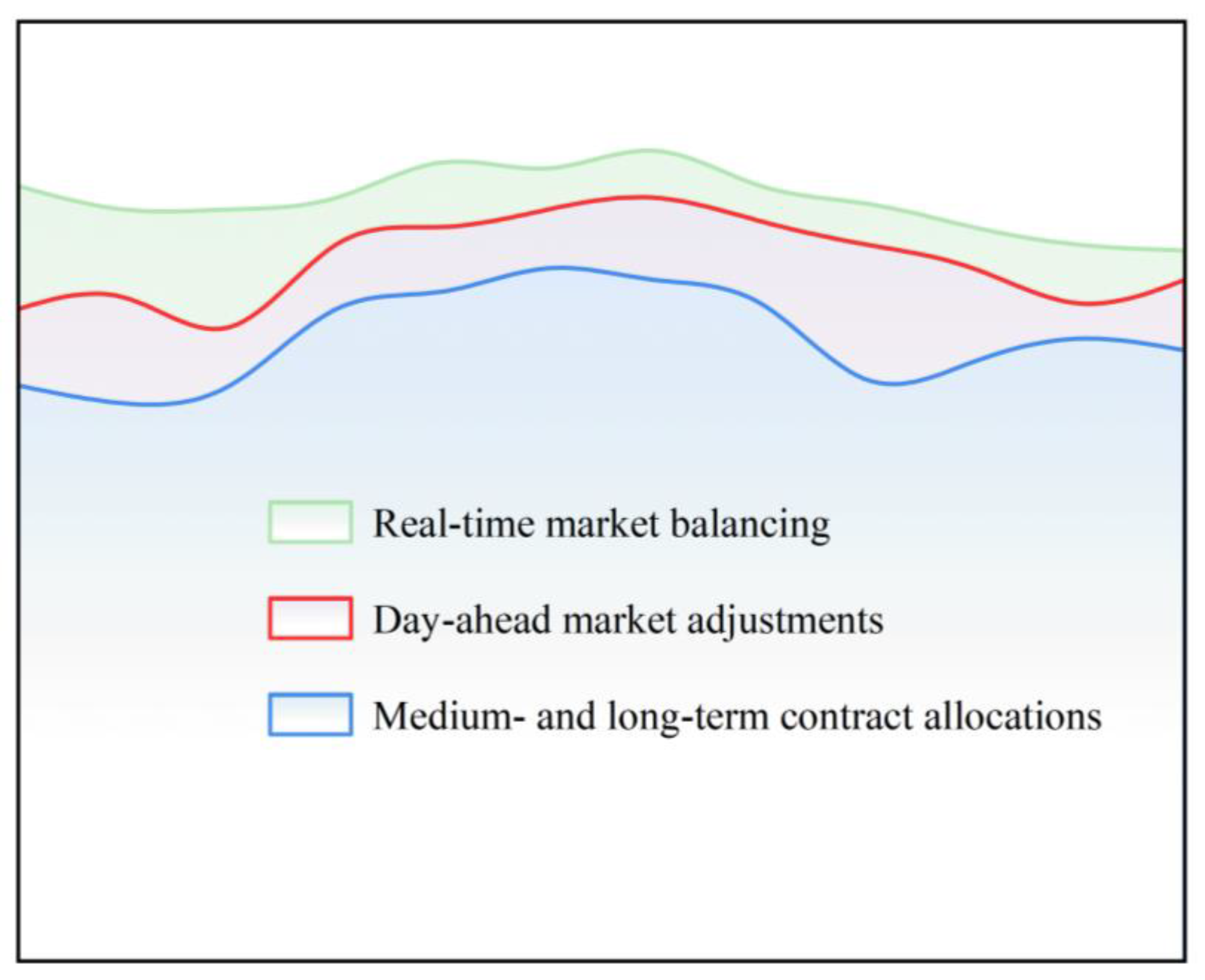
2.1. Theoretical Analysis of Cascade Hydropower Stations’ Participation in the EEM

As shown in Figure 2, in the power generation sector, daily electricity settlements are structured around three primary components:

• Medium- and long-term contract allocations: These are based on energy sales agreements established through trading platforms, providing a foundational generation schedule.
• Day-ahead market adjustments: To align with real-time grid demands and supply conditions, adjustments are made in the day-ahead market, ensuring a balanced and responsive generation plan [23].
• Real-time market balancing: Any discrepancies between forecasted and actual loads are addressed in the real-time market, facilitating immediate market-based corrections to maintain system equilibrium [24].

Figure 2. Diagram of the relationship between the various levels of the market under EEM.

Figure 2. Diagram of the relationship between the various levels of the market under EEM.

For cascade hydropower stations, daily electricity settlements encompass these three segments, ensuring comprehensive and adaptive participation in the EEM [25].

2.2. Theoretical Analysis of Cascade Hydropower Stations’ Participation in the PRM

In the power auxiliary services market [26], the principle of “those who provide the service gain; those who benefit bear the cost” is applied. Specifically, generating units that offer deep-peaking services receive compensation, while units that do not fulfill this obligation share the associated costs [27]. For hydropower plants participating in the PRM, there are two scenarios:

• Participating in deep peaking to earn compensation.
• Contributing to the shared costs when thermal power units engage in deep peaking.

To maximize the benefits of cascade hydropower stations in the PRM, increasing peaking compensation within a reasonable range and reducing peaking cost allocation is essential.

As shown in Figure 3a, during this period, the generating units connected to the grid included hydropower, thermal power, wind power, and photovoltaic (PV) power stations. When wind and PV generation experience a surge while the load demand remains low, hydropower and thermal power units must reduce their output. If the output falls below the compensated peaking threshold, both hydropower and thermal power units participate in deep peaking. Meanwhile, the reduction in generation from hydropower and thermal units due to peaking participation results in financial losses, which are jointly borne by the wind and PV power stations operating in the same period.

The generating side’s compensation benefits and peaking cost allocation for participating in the peak market are given in the following equation:

$$\left\{\begin{array}{l}{Z}_h=\eta \cdot Y_h\cdot \Delta t\\ Z_f=\eta \cdot Y_f\cdot \Delta t\\ Z_w=\eta \cdot Y_w\cdot \Delta t\\ Z_s=\eta \cdot Y_s\cdot \Delta t\\ Z_h+Z_f=Z_w+Z_s\end{array}\right.$$

(1)

$Z_h$ and $Z_f$ are the compensating revenues from hydropower and thermal power; $Z_w$ and $Z_s$ are the peak-sharing expenditures from wind power and PV; $\eta$ is the compensation tariff during the period; $Y_h$ and $Y_f$ are the peaking capacity contributed by hydropower and thermal power, respectively; $Y_w$ and$Y_s$ are the additional feed-in electricity from wind power and PV, respectively.

As shown in Figure 3b, when thermal power participates in deep peaking while hydropower, wind power, and photovoltaic power are generated during the same period, the peaking compensation received by thermal power due to deep peaking is shared among the other three power sources.

The generating side’s compensation benefits and peaking cost allocation for participating in the PRM are given in the following equation:

$$\left\{\begin{array}{l}{Z}_f=\eta \cdot Y_f\cdot \Delta t\\ Z_h=\eta \cdot Y_h\cdot \Delta t\\ Z_w=\eta \cdot Y_w\cdot \Delta t\\ Z_s=\eta \cdot Y_s\cdot \Delta t\\ Z_f=Z_h+Z_w+Z_s\end{array}\right.$$

(2)

$Z_f$ is the compensating gain for thermal power; $Z_h$, $Z_w$, and $Z_s$ are the peak-sharing expenditures for hydropower, wind, and PV; $\eta$ is the compensatory tariff in that time period; $Y_f$ is the peaking capacity contributed by thermal power; $Y_h$, $Y_w$, and $Y_s$ are the new feed-in electricity added by hydropower, wind power, and PV, respectively.

3. Economic Dispatch Model for Cascade Hydropower Stations Considering the EEM and PRM

The strategy sets a total of five objective functions: maximizing the generation of cascade hydropower stations, maximizing the benefits from the EEM, minimizing the impact of the spot market, maximizing the compensation revenue from peak regulation, and minimizing the peaking cost allocation for peak regulation. A multi-objective joint dispatch strategy is used to solve these objective functions. By considering constraints from the hydropower station itself, transmission capacity limitations, and the perspective of the electricity market, this strategy aims to achieve the maximization of the economic benefits of cascade hydropower stations.

3.1. Objective Function

Objective 1: Maximizing the power generation of cascade hydropower stations

$$W_E={\displaystyle \sum _{i=1}^I{\displaystyle \sum _{t=1}^T({\eta }_i}}\cdot Q_i^t\cdot H_i^t\cdot \Delta t)$$

(3)

$W_E$ is the intraday generation of the cascade hydropower station; $T$ is the total duration of 24 h; $i$ is the labeling number of each station; $Q_i^t$ is the generation flow rate of $i$ station at moment $t$; $H_i^t$ is the average net head of the generation of the $i$ station at moment $t$; $I$ is the total number of cascade hydropower stations; $\Delta t$ is the number of hours.

Objective 2: Maximizing the benefits of cascade hydropower station participation in the EEM

(1)

Medium- and long-term market returns:

$$W_C=C_l{\displaystyle \sum _{t=1}^T{E}_l^t}$$

(4)

$W_C$ is the revenue of the cascade hydropower station in the medium- and long-term market, $C_l$ is the price of electricity sold in the signed medium- and long-term contract, and $E_l^t$ is the amount of electricity disaggregated by the medium- and long-term contract to each period in period $t$.

(2)

Day-ahead market returns:

$$W_d={\displaystyle \sum _{t=1}^T{C}_d^t(E_d^t}-E_l^t)$$

(5)

$W_d$ is the revenue of cascade hydropower stations in the day-ahead market, $C_d^t$ is the price of electricity sold in each time slot, and $E_d^t$ is the amount of electricity generated by the cascade hydropower station in each time slot.

(3)

Real-time market returns:

$$W_r={\displaystyle \sum _{t=1}^T{C}_r^t}(E_r^t-E_d^t)$$

(6)

$W_r$ is the revenue of cascade hydropower stations in the real-time market, $C_r^t$ is the price of electricity sold in the real-time market every 15 min, and $E_r^t$ is the amount of electricity generated by cascade hydropower stations in each time period allocated under the electricity trading platform.

$$Max{W}_a={\displaystyle \sum _{n=1}^N{W}_C+W_d+W_r}$$

(7)

$W_a$ is the combined revenue of the EEM.

Objective 3: Maximization of compensation benefits from the participation of cascade hydropower stations in the PRM

Section 2.2 provides a detailed description of the mechanisms of compensation benefits from the participation of cascade hydropower stations in the PRM and analyzes the peak regulation output characteristics of cascade hydropower stations. From Section 2.2:

$$W_s={\eta }_s\cdot Y_s$$

(8)

$Y_s$ is the output of cascade hydropower stations in the PRM; ${\eta }_s$ is the PRM compensation price.

$$Max{W}_b={\displaystyle \sum _{t=1}^T{W}_S}\cdot \Delta t_1$$

(9)

$W_b$ is the compensatory return of cascade hydropower stations in the PRM.

Objective 4: Cascade hydropower stations are least negatively impacted by the spot market

Wind and solar power, as the primary participants in the spot market, contribute to increased market supply, particularly in regions with abundant wind and solar resources. However, the transmission capacity in different regions is limited. To better accommodate wind and solar power, hydropower output may be reduced to some extent. Additionally, since wind and solar power have lower marginal prices, their participation in the spot market can impact the market-clearing price of hydropower. The decline in hydropower’s grid electricity price due to the presence of wind and solar power in the spot market may further propagate to the medium- and long-term markets, affecting the contracted electricity transactions of cascade hydropower stations. In extreme cases, this could significantly undermine the economic benefits of cascade hydropower generation.

In the spot market, electricity prices are determined by wind, solar, thermal power, and demand levels. However, the inherent uncertainty of wind and solar power generation introduces price volatility. Assuming the baseline electricity price for a given period is $X_B$, the fluctuating component of the price can be denoted as $\Delta x$.

Then, the actual price of grid-connected electricity is $X_T=X_B+\Delta x$, while the fluctuating price of electricity $\Delta x$ depends on the mean load $\overline{P_l}$ in that time period, and the average outputs of wind, PV, and thermal power in that time period are $\overline{E_{W,t}},\overline{E_{S,t}},\overline{E_{f,t}}$.

$$\Delta x=Y((\overline{E_{W,t}}+\overline{E_{S,t}}+\overline{E_{f,t}})-\overline{P_l})$$

(10)

$Y$ represents the nonlinear relationship between fluctuating electricity prices, the power output of various types of power plants, and load, which is derived from historical data fitting.

When $\Delta x$ > 0, electricity prices are relatively high to some extent. In this case, cascade hydropower stations can increase power generation and feed more electricity into the grid to maximize their economic benefits. Conversely, when $\Delta x$ < 0, electricity prices are lower, and cascade hydropower stations can choose to store water while meeting peak regulation requirements. As $\Delta x$ fluctuates, optimizing the power output of cascade hydropower stations can help improve their overall generation efficiency and economic returns.

Once a cascade hydropower station has met its allocated electricity target under medium- and long-term contracts, the variation in power generation due to fluctuations in $\Delta x$ is given by $\Delta E_{h,t}$.

Then, the objective function is minimized by the negative impact of the spot market as the product of the amount of power change and the fluctuating electricity price in the spot market.

$$W_C=Min{\displaystyle \sum _{n=1}^N{\displaystyle \sum _{t=1}^T\Delta E_{h,t}}}\cdot \Delta x$$

(11)

$\Delta x$ is the fluctuating price of electricity; $\Delta E_{h,t}$ is the variation in power generation.

Objective 5: Minimizing the peaking cost allocation for cascade hydropower stations in the PRM

In power systems, all grid-connected power plants are obligated to participate in grid-peaking operations. Power units undertaking deep-peaking responsibilities receive compensation for providing peaking ancillary services, while those not fulfilling this obligation must share the associated peaking service costs. The cost of deep-peaking compensation is allocated among all market participants based on their electricity generation during the corresponding period.

From the perspective of maximizing the economic benefits of cascade hydropower stations, it is advantageous to minimize power generation during periods of high peak demand in the grid. This strategy effectively reduces the share of peaking cost allocation borne by hydropower units.

Thermal power plants serve as the primary providers of deep-peaking services, and their reduction in power output during peaking periods is denoted as $E_{F,t}$. The initially scheduled output of the cascade hydropower unit is $P_{H,t}$. To reduce the peak cost allocation, the hydropower station can adjust its output by reducing its scheduled generation by a decision variable $\Delta P_{H,t}$. Thus, optimizing $\Delta P_{H,t}$ allows cascade hydropower stations to strategically lower their share of peaking cost allocation.

$$W_D=Min{\displaystyle {\sum }_{i=1}^I{\displaystyle {\sum }_{t=1}^T(C_{F,t}}}\cdot E_{F,t}\cdot {\displaystyle \frac{\Delta P_{H,i}}{P_{F,i}+P_{S,i}+P_{w,i}+P_{H,i}}})$$

(12)

$P_{F,i}$, $P_{S,i}$, $P_{w,i}$, and $P_{H,i}$ are the output of thermal power, photovoltaic power, wind power, and the original plan of on-grid hydropower in the time period, $E_{F,t}$ is the pressure output of thermal power to participate in peaking, and $C_{F,t}$ is the negotiated electricity price for this time period.

$$Max{E}_A={\lambda }_1{W}_E+{\lambda }_2{W}_a+{\lambda }_3{W}_b-{\lambda }_4{W}_c-{\lambda }_5{W}_d$$

(13)

${\lambda }_1$, ${\lambda }_2$, ${\lambda }_3$, ${\lambda }_4$, and ${\lambda }_5$ are the weight coefficients of the respective objective functions.

The optimization scheduling problem of hydropower plants is addressed by simultaneously using the Analytical Hierarchy Process (AHP) to convert multi-objective functions into a single-objective function. This paper focuses on coordinating the optimization of five objectives: the generation capacity of the cascade hydropower stations, the benefits of the EEM, the compensatory benefits of peaking, the influence of the spot market and the peaking cost allocation, and the performance of a weight analysis for these objectives. To achieve the normalization of multiple objectives and unify their dimensions, this paper employs a judgment matrix to weigh the importance of each objective.

The judgment matrix can be further obtained based on the judgment elements obtained:

$$M=\left(\begin{array}{ccc}{C}_{11}& \cdots & C_{1n}\\ ⋮& \ddots & ⋮\\ C_{n1}& \cdots & C_{nn}\end{array}\right)$$

(14)

$n$ is the number of objectives in this matrix; $M$ is the judgment matrix.

After determining the matrix $M$, it is possible to derive the ratio of each objective function:

$${\pi }_i={\left({\displaystyle \prod _{j=1}^n{C}_{ij}}\right)}^{{\displaystyle \frac{1}{n}}}$$

(15)

The weights of the objectives are given in the following equation:

$${\lambda }_i={\displaystyle \frac{{\pi }_i}{{\displaystyle \sum _{j=1}^n{\pi }_j}}}$$

(16)

The objective function $E_A$ is to maximize the economic benefits of cascade hydropower stations, and ${\lambda }_1\sim {\lambda }_5$ represents the weight coefficient of the objective function. The different weight coefficients are set by evaluating the importance of the five objective functions.

$${\lambda }_1+{\lambda }_2+{\lambda }_3+{\lambda }_4+{\lambda }_5=1$$

(17)

3.2. Constraint Condition

(1)

Water level constraints:

$$Z_{i,\min }<Z_i^t<Z_{i,\max }$$

(18)

$Z_{i,\min }$ and $Z_{i,\max }$ represent the lower and upper water level limits of the $i$th hydropower station, respectively, while $Z_i^t$ denotes the water level of the $i$th hydropower station at a time.

(2)

Water balance constraints:

$$\begin{array}{l}{V}_{i,t}=V_{i,t-1}+\left(I_{i,t}+Q_{out,i-1,i-{\tau }_i}-Q_{out,i,t}\right)\Delta t\end{array}$$

(19)

In the equation, $V_{i,t}$ represents the reservoir storage of hydropower station i at the end of period t; $I_{i,t}$ denotes the inflow to station i during period t; $Q_{out,i,t}$ represents the outflow from station i during period t; τ_i is the travel time for the outflow from the upstream station to reach the downstream station.

(3)

Transmission channel constraints:

$${\displaystyle \sum _{i=1}^{N_G}\left(P_{pv,i,t}+P_{i,t}\right)}\le P_{D,\max },i\in D_G$$

(20)

In the equation, $D_G$ represents the set of subordinate power stations in the interconnected transmission line, while $P_{D,\max }$ denotes the maximum transmission capacity.

(4)

Medium- and long-term contracted power decomposition constraints:

$${\displaystyle \sum _{t=1}^T{E}_l^t}\ge E_{basic,l}^t$$

(21)

In the equation, $E_l^t$ represents the contracted electricity allocated to each day from medium- and long-term agreements, while $E_{basic,l}^t$ denotes the minimum daily electricity generation.

(5)

Hydropower plant output constraints at all levels:

$$P_{i,\min }<P_i^t<P_{i,\max }$$

(22)

$P_{i,\min }$ and $P_{i,\max }$ represent the lower and upper power output limits of the hydropower station, respectively.

(6)

Upper and lower limits of reservoir capacity and flow rate constraints for hydropower plants at all levels:

$$\left\{\begin{array}{l}{V}_{i,\min }\le V_{i,t}\le V_{i,\max }\\ Q_{out,i,\min }\le Q_{out,i,t}\le Q_{out,i,\max }\end{array}\right.$$

(23)

In the equation, $V_{i,\min }$ and $V_{i,\max }$ represent the minimum and maximum reservoir storage of a hydropower station, respectively, while $Q_{out,i,\min }$ and $Q_{out,i,\max }$ denote the minimum ecological outflow and the maximum outflow of a station, respectively.

4. An Economic Dispatch Model Solution Based on the HHO Algorithm

4.1. Fundamentals of the HHO Algorithm

In the optimal scheduling problem of cascade hydropower stations, the HHO algorithm is capable of handling complex nonlinearities, discontinuities, multi-modal, and high-dimensional issues. Additionally, it can prevent premature convergence, leading to better outcomes when solving multi-objective optimization problems. Therefore, this algorithm is employed to solve the model.

The Harris Hawk Optimization (HHO) algorithm is a metaheuristic algorithm that simulates the hunting behavior of Harris hawks in nature [28]. The algorithm primarily consists of two phases: exploration and exploitation, with a transition between the two phases governed by the prey’s escape energy. In the exploration phase, Harris hawks explore potential search areas by observing their environment and exchanging information with other individuals in the population. During the exploitation phase, the HHO algorithm adopts four different strategies to launch attacks based on the prey’s condition [29]. The basic description of the Harris Hawk Optimization algorithm is as follows [30]:

(1)

Global exploration phase

When the prey’s escape energy is $\left|E\right|\ge 1$, the algorithm enters the global exploration mode. This phase primarily occurs during the early iterations. In this stage, a random number $\alpha$ is generated. When $\alpha \ge 0.5$, the hawks have not located the prey, so they randomly update their positions. However, when $\alpha <0.5$, the hawks have detected the prey, and they update their positions based on the location of the prey.

$$X(t+1)=\left\{\begin{array}{l}{X}_{prey}(t)-X_m(t)-r_3\cdot \left[(LB+r_4\cdot (UB-LB)\right.]\hspace{1em}\hspace{1em}\alpha <0.5\\ X_{rand}(t)-r_1\cdot |X_{rand}(t)-2r_2\cdot X(t)|\hspace{1em}\hspace{1em}\hspace{1em}\hspace{1em}\hspace{1em}\hspace{1em}\hspace{1em}\alpha \ge 0.5\end{array}\right.$$

(24)

$X_{prey}(t)$ is the position of the prey, $X_m(t)$ is the average position of the population of hawks, $X_{rand}(t)$ is the position of a randomly selected hawk, $UB$ and $LB$ are the upper and lower bounds of the search range. $r_1$~$r_4$ are random numbers.

(2)

Transition phase

$$C=1-{\displaystyle \frac{t}{T}}$$

(25)

$t$ represents the current iteration number, and $T$ is the maximum iteration number. As the number of iterations increases, a linear relationship is established, causing $C$ to gradually decrease from 1 to 0.

$$E=2E_{0}C$$

(26)

$E$ represents the prey’s escape energy, and $E_0$ is the initial escape energy. This phase is used to transition between the exploration and exploitation stages.

(3)

Development phase

When $0.5<\left|E\right|<1$ is true, it indicates that the prey still has energy, so a soft encirclement or a rapid dive soft encirclement are employed.

• Soft Surrounding

When $0.5<\left|E\right|<1$ and $P\ge 0.5$, $P$ represents the prey’s escape probability. In this case, the prey has no possibility of escaping.

$$X(t+1)=[X_{prey}(t)-X(t)]-E\cdot |\beta \cdot X_{prey}(t)-X(t)|$$

(27)

$\beta$ is the random jump strength of the prey. $X_{prey}(t)$ is the position of the prey. $X(t)$ is the actual location of the eagle population at the iteration.

2.

Quick Dive Soft Wrap

When $0.5<\left|E\right|<1$ and $P<0.5$, the prey has a possibility of escape.

$$X(t+1)=\left\{\begin{array}{l}U=X_{prey}(t)-E\ast |\beta X_{prey}(t)-X(t)| \hspace{1em}\hspace{1em}\hspace{1em}\hspace{1em}\mathrm{F}\left(\mathrm{u}\right)\mathrm{F}\left(\mathrm{x}\right(\mathrm{t}\left)\right)\\ V=U+S\ast Levy(D)\hspace{1em}\hspace{1em}\hspace{1em}\hspace{1em}\hspace{1em}\hspace{1em}\hspace{1em}\hspace{1em}\hspace{1em} \mathrm{F}\left(\mathrm{v}\right)\mathrm{F}\left(\mathrm{x}\right(\mathrm{t}\left)\right)\end{array}\right.$$

(28)

When the escape energy is less than 0.5, Lévy flight is introduced to simulate the irregular behavior of the prey’s escape. The resulting position $U$ is compared with the current position’s fitness. If the outcome is suboptimal, the position is gradually adjusted until the best position is selected. $Levy(D)$ is the Lévy flight strategy, and $S$ is a D-dimensional random vector.

3.

Hard Surround

When $\left|E\right|<0.5$ and $P\ge 0.5$,

$$X(t+1)=X_{prey}(t)-E\cdot (X_{prey}(t)-X(t))$$

(29)

4.

Rapid Dive Hard Surround

When $\left|E\right|<0.5$ and $P<0.5$,

$$X(t+1)=\left\{\begin{array}{l}U=X_{prey}(t)-E\ast |\beta X_{prey}(t)-X_m(t)|\hspace{1em}\hspace{1em} \mathrm{F}\left(\mathrm{u}\right)\mathrm{F}\left(\mathrm{x}\right(\mathrm{t}\left)\right)\\ V=U+S\ast Levy(D)\hspace{1em}\hspace{1em}\hspace{1em}\hspace{1em}\hspace{1em}\hspace{1em}\hspace{1em}\hspace{1em} \mathrm{F}\left(\mathrm{v}\right)\mathrm{F}\left(\mathrm{x}\right(\mathrm{t}\left)\right)\end{array}\right.$$

(30)

$Levy(D)$is the Lévy flight strategy, and $S$ is a D-dimensional random vector. $X_{prey}(t)$ is the position of the prey, $X_m(t)$ is the average position of the population of hawks, and $\beta$ is the random jump strength of the prey. $E$ represents the prey’s escape energy. $F(·)$ is the fitness function.

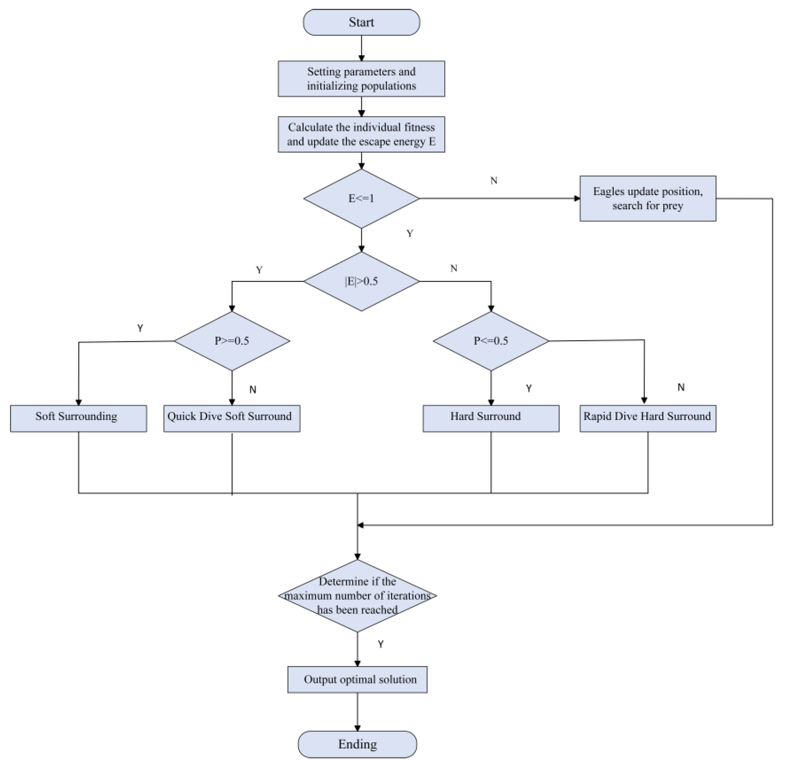
4.2. HHO Algorithm Solution Flow

As shown in Figure 4, the diagram illustrates the basic process of the Harris Hawk Optimization algorithm for solving a model.

(1)

Use the parameters of the cascade hydropower stations and the power grid as input data for the scheduling model; set the size of the hawk population and the total number of iterations.

(2)

Randomly initialize the population positions and calculate the fitness values of each hawk in the population.

(3)

Update the prey’s escape energy based on Equation (26).

(4)

Determine whether the hawks enter the exploration phase or the exploitation phase based on the prey’s escape energy.

(5)

When $E|\ge 1$, the prey’s escape energy is high, so the population’s positions are updated according to Equation (24), and the hawks update their positions, entering the exploration phase.

(6)

When $\left|E\right|<1$, the hawks update their positions, entering the exploitation phase.

(7)

When $\left|E\right|>0.5$, the escape probability is used to determine whether to employ a soft encirclement or a progressive soft encirclement.

1.

When $P\ge 0.5$, update the position based on Equation (27).

2.

When $P<0.5$, update the position based on Equation (28).

(8)

When $\left|E\right|<0.5$, the escape probability is used to determine whether to employ a hard encirclement or a progressive hard encirclement.

3.

When $P\ge 0.5$, update the position based on Equation (29).

4.

When $P<0.5$, update the position based on Equation (30).

(9)

Finally, check whether the maximum iteration count has been reached. If the maximum iteration count is reached, output the optimal solution; if not, return to step (3) and continue the iterations.

5. Simulation Verification

5.1. Initial Data for Simulation

To verify the effectiveness of the scheduling strategy proposed in this paper, a case study of the cascade hydropower station scheduling system is considered, which includes three hydropower stations, two photovoltaic plants (with installed capacities of 500 MW and 500 MW), one wind power plant (with an installed capacity of 1000 MW), and one thermal power plant (with an installed capacity of 3000 MW).

Table 1. Basic data table for cascade hydropower stations.

Project	Hydropower Station A	Hydropower Station B	Hydropower Station C
Average annual runoff (billion m3)	94.4	127	138
Average annual flow (m3/s)	299	403	436
Normal storage level(m)	400	200	80
Dead water level (m)	350	180	78
Total reservoir capacity (billion m3)	45.8	33.4	4.89
Reservoir regulation performance	Multi-annual regulation	Annual regulation	Daily regulation
Installed capacity (MW)	1840	1212	270
Firm power (MW)	308.3	241.9	77.4
Maximum head (m)	202	122	40
Minimum head (m)	147	80.7	22.3

presents the key parameters of the cascade hydropower stations. Additionally, since the scheduling of cascade hydropower stations largely depends on the water inflow conditions, simulations are conducted under two scenarios: the wet and dry seasons.

This section establishes four dispatch schemes to evaluate the impact of the EEM and PRM on the economic dispatch of cascade hydropower stations. Scheme 1 considers cascade hydropower stations participating only in the EEM. Scheme 2 considers the spot market’s influence on the power output of cascade hydropower stations in the energy market. Scheme 3 further incorporates the participation of cascade hydropower stations in both the energy market and the ancillary peak regulation market under the influence of the spot market. Based on Scheme 3, Scheme 4, which represents the proposed dispatch strategy, additionally considers the cost-sharing mechanisms of the cascade hydropower stations in the PRM.

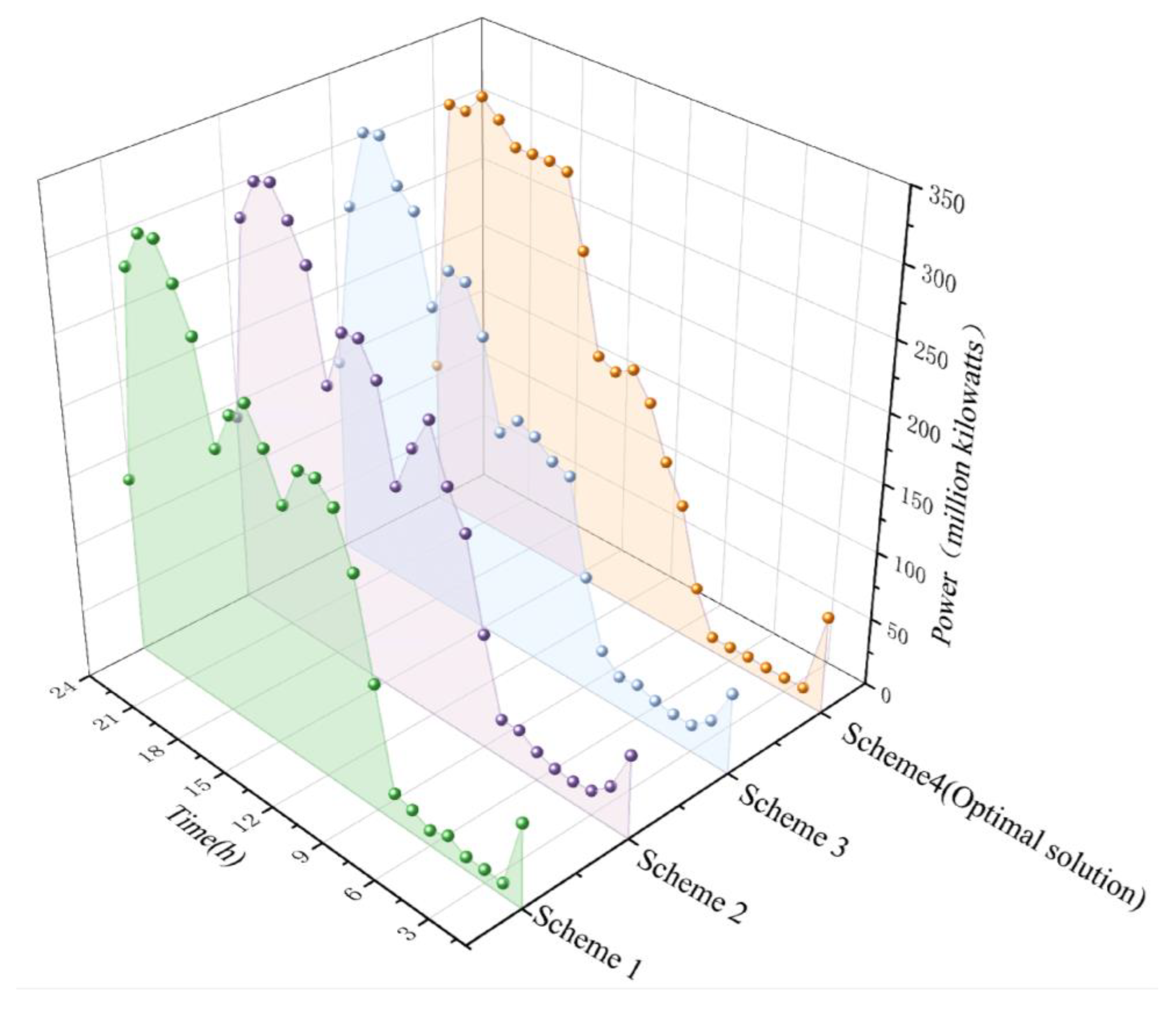
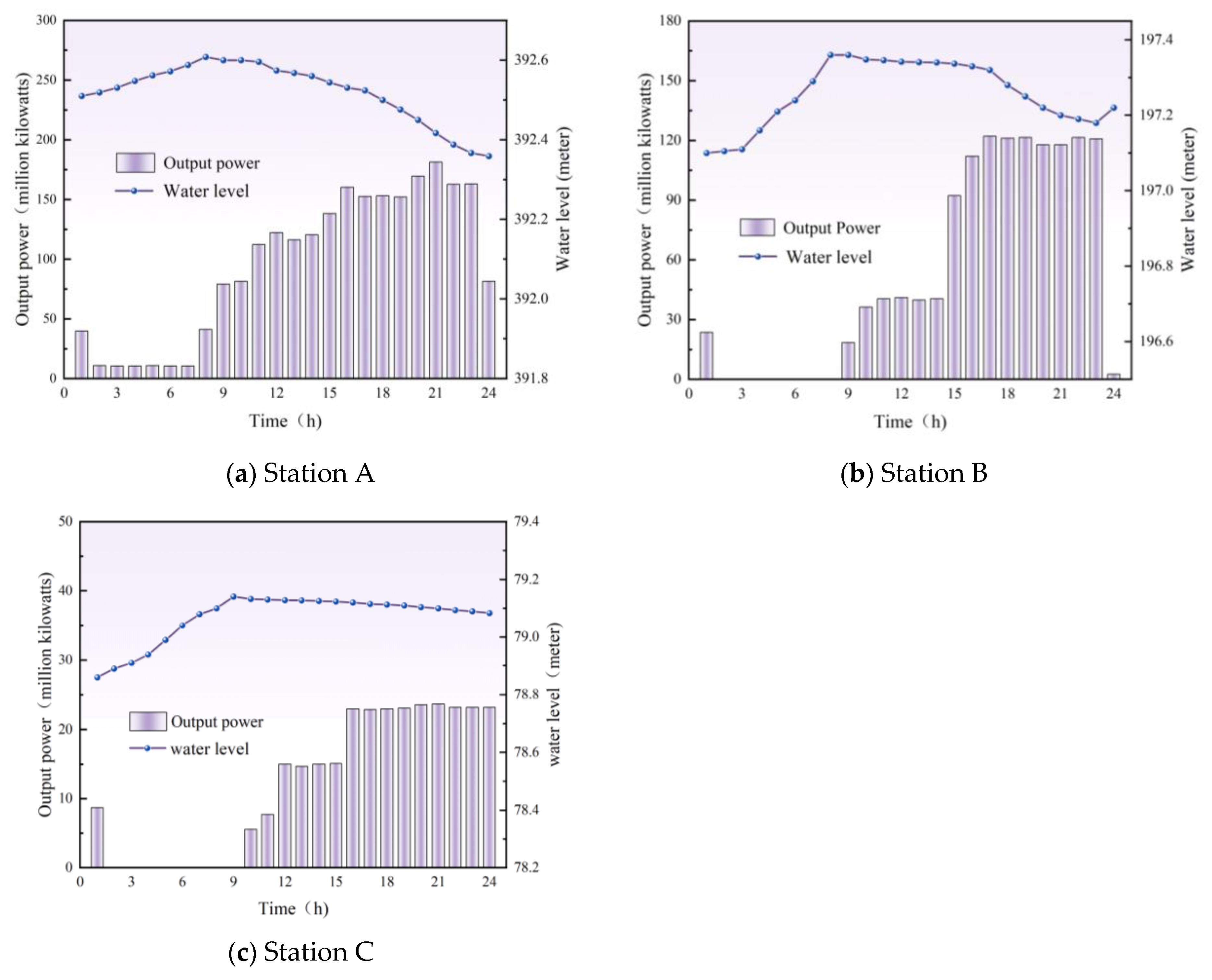
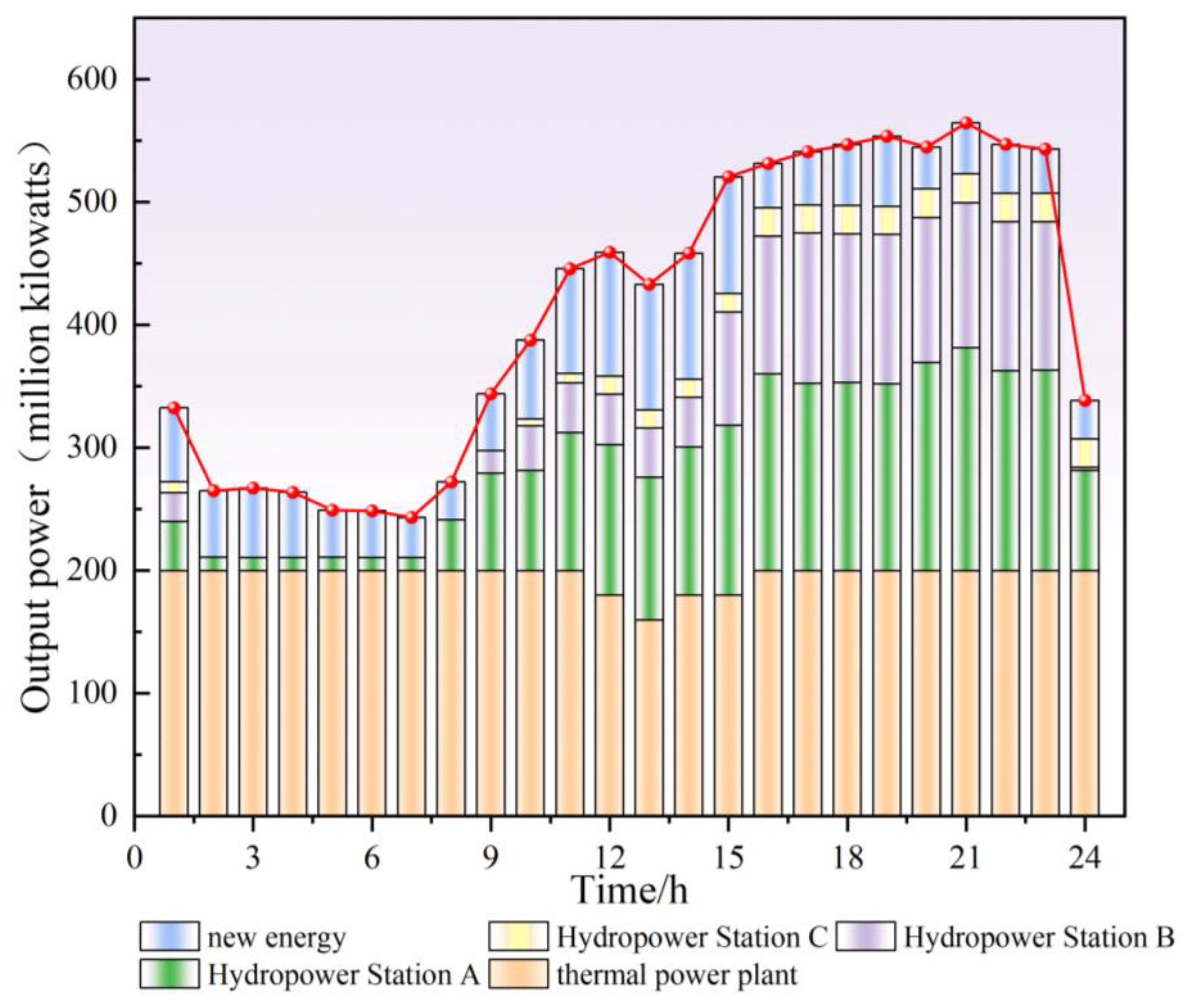
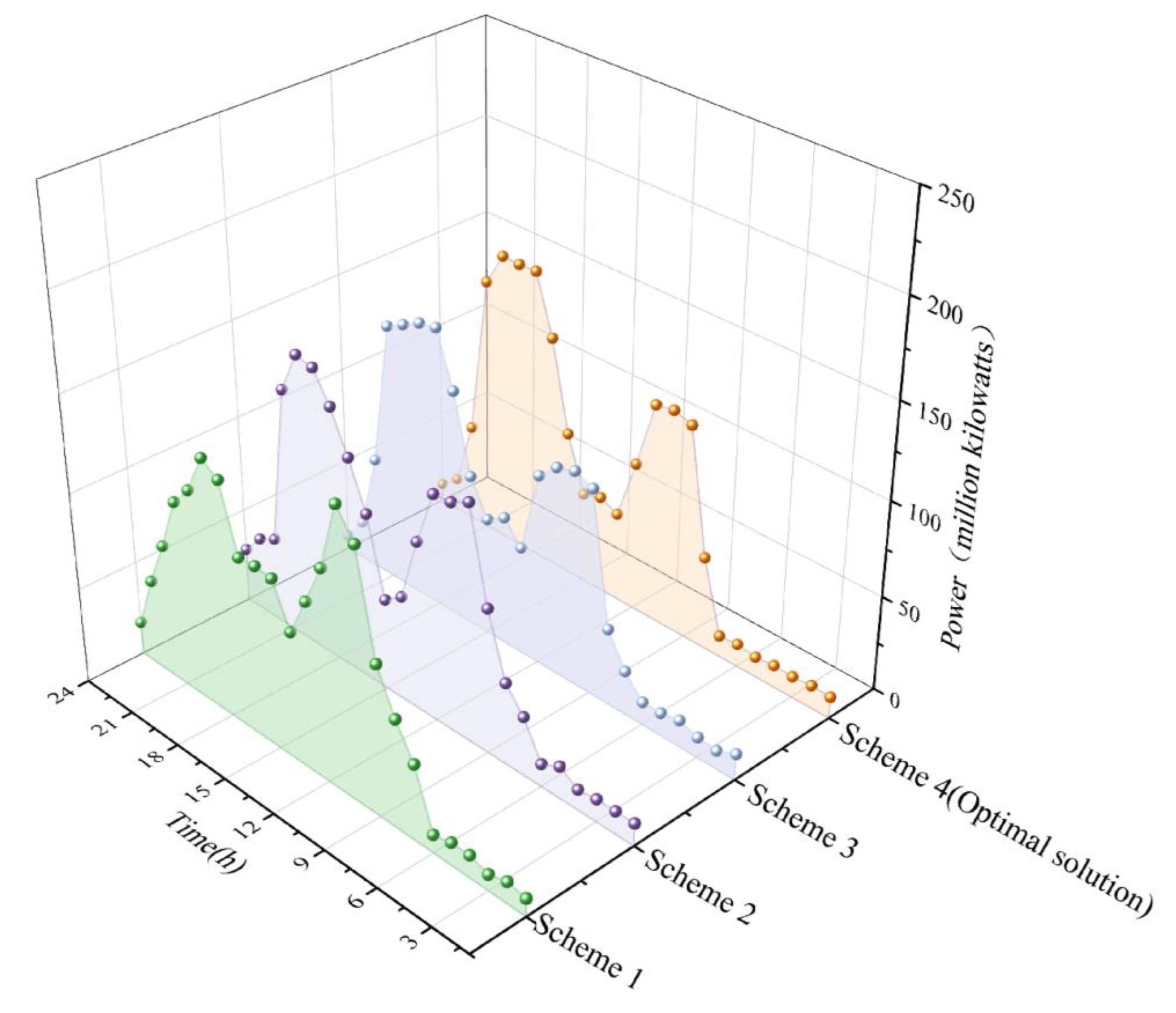
5.2. Simulation Results of Cascade Hydropower Stations Under the Wet Season

Based on the above scenarios, a comparison of the output of cascade hydropower stations under different scenarios during the wet season is derived using 24 h a day as a unit.

As illustrated in Figure 5, the power output of cascade hydropower stations varies under different dispatch schemes. Scheme 2, compared to Scheme 1, additionally accounts for the influence of the spot market. Given the abundant photovoltaic (PV) resources in the cascade hydropower basin, PV generation peaks around midday. To enhance the overall economic efficiency of cascade hydropower stations, their generation is strategically reduced during this period to facilitate water storage. In the evening, when electricity demand reaches its daily peak and PV generation is unavailable, hydropower stations increase their output to maximize economic returns. Scheme 3 builds upon Scheme 2 by integrating peak regulation market (PRM) participation. Positive peak regulation allows cascade hydropower stations to generate additional electricity, while deep-peak regulation provides financial compensation when renewable energy generation surges. Under Scheme 3, hydropower stations participate in the PRM at midday, further reducing their generation compared to Scheme 2 but receiving compensation from the ancillary service market. Additionally, during the evening peak, the availability of stored water enables higher power generation, allowing hydropower stations to contribute to peak load regulation and achieve greater overall revenue than in Scheme 2. Scheme 4, the proposed dispatch strategy, extends Scheme 3 by incorporating a cost-sharing mechanism for peak regulation. During the early morning hours, when electricity demand is low and wind power generation is strong, thermal power plants are prioritized for peak regulation to accommodate renewable energy. The compensation for thermal power regulation is distributed among other generating units operating during this period. To minimize cost-sharing expenses and enhance overall economic efficiency, cascade hydropower stations strategically reduce their generation during these hours, thereby increasing their total revenue.

As shown in

Table 2. Revenue table for hydropower stations under different schemes during the wet season.

Scheme	Revenue from EEM/CNY	Revenue from PRM/CNY	Total Revenue /CNY
Scheme 1	1376.45	0	1376.45
Scheme 2	1389.34	0	1389.34
Scheme 3	1332.89	66.34	1399.23
Scheme 4 (optimal scheme)	1321.23	81.52	1402.75

, The specific revenue outcomes of cascade hydropower stations under different schemes are as follows. Scheme 2 yields slightly higher revenue in the EEM than Scheme 1 due to the consideration of spot market price fluctuations. However, neither Scheme 1 nor Scheme 2 generate revenue from the PRM.

In contrast, Scheme 3 and Scheme 4 engage in peak regulation, resulting in a decrease in electricity generation. However, they offset this loss by earning revenue from the PRM. Consequently, their overall revenue is higher than the first two schemes. Furthermore, since Scheme 3 produces a greater power output than Scheme 4 during thermal power peak regulation, it incurs higher cost-sharing expenses. Therefore, the proposed optimization strategy in Scheme 4 ultimately achieves the highest total revenue among all four schemes.

Figure 6 presents the output strategy and water level control strategy for the cascade hydropower stations according to the optimal scheme.

As shown in Figure 6, since the cascade hydropower stations are in the high-flow period, they can generally operate at full capacity during the evening peak. However, during the midday peak, due to transmission capacity limitations, a certain degree of peak regulation is implemented to reserve a sufficient margin for renewable energy generation, reducing the curtailment of wind and solar power. This results in a reduction in hydropower output to store water for the evening peak. During the early morning hours, when electricity demand is low, and wind power is high, the cascade hydropower stations operate at a low output level.

Figure 7 presents the power output of various power plants under the optimal dispatch strategy.

Through the coordination between the power grid and cascade hydropower stations, the optimal dispatch strategy ensures the full consumption of renewable energy while smoothing the thermal power generation curve, optimizing thermal power operation, and enhancing the revenue of cascade hydropower stations.

First, the optimal scheme increases the dispatchable power of cascade hydropower stations during peak hours, strengthening their peak-shaving capability during both the morning and evening peaks. During high renewable energy generation periods, cascade hydropower stations participate in deep-peak regulation, earning compensation from PRM while reducing the peak regulation demand of thermal power.

Additionally, during the midday peak, although wind power is not at its optimal resource availability, the overall renewable energy output reaches its peak due to high photovoltaic generation. As a result, cascade hydropower stations reduce their output to prioritize the transmission of renewable energy, thereby facilitating its full utilization.

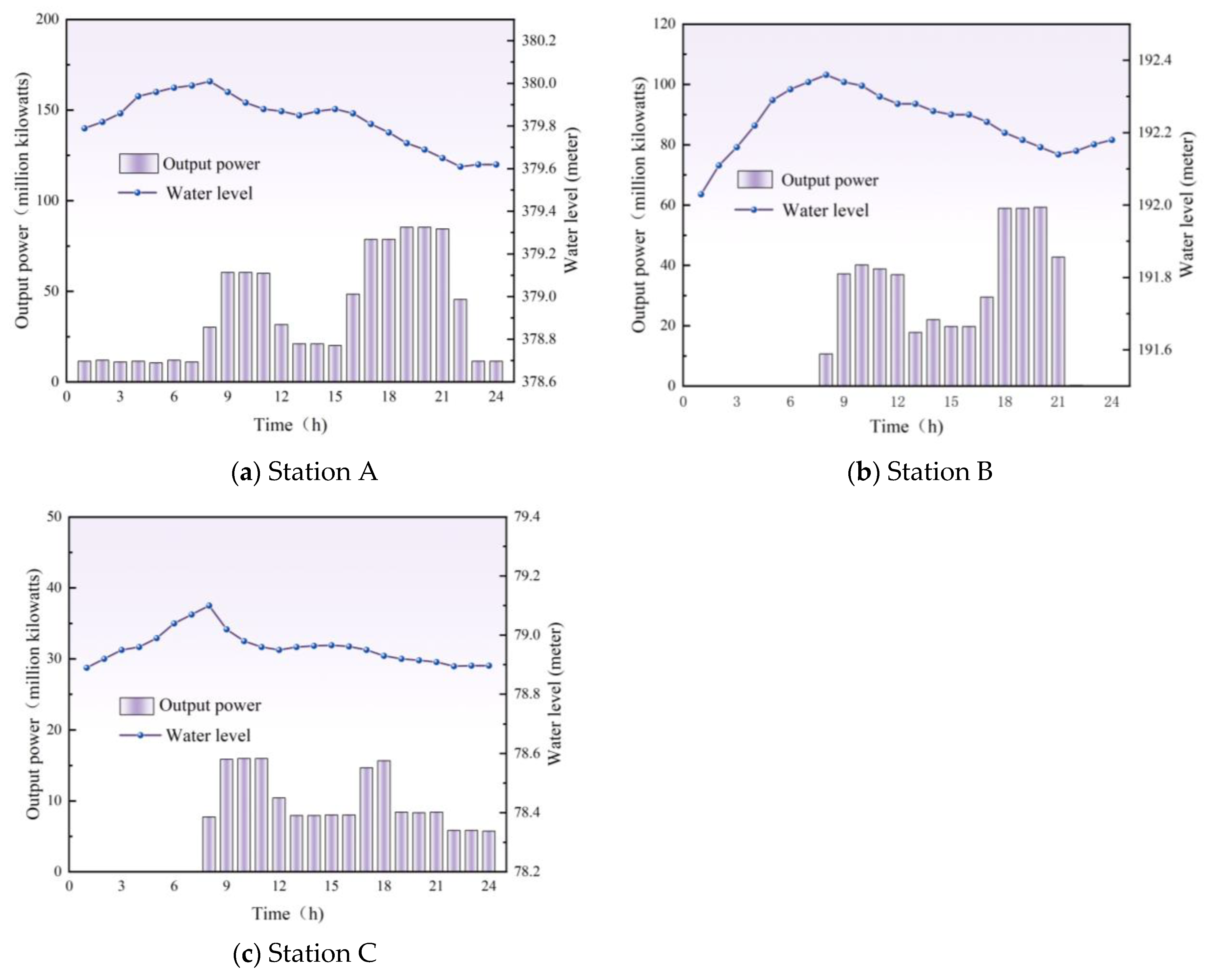
5.3. Simulation Results of Cascade Hydropower Stations Under the Dry Season

As shown in Figure 8, the power output comparison under different schemes during the low-flow period is presented. Scheme 1 exhibits a slightly higher output between 15:00 and 18:00; however, due to the impact of low-flow conditions, its output is insufficient during the evening peak. Scheme 2, building upon Scheme 1, considers the influence of the spot market by reducing the output of cascade hydropower stations during midday to avoid periods of high renewable energy generation. Scheme 3 further participates in peak regulation during low-load periods, reducing output but gaining compensation from the PRM. Scheme 4 strategically reduces output during midday when renewable energy generation peaks to avoid the cost-sharing burden caused by thermal power plants’ peak regulation, thereby minimizing additional expenses.

As shown in

Table 3. Revenue table for hydropower stations under various schemes during the dry season.

Scheme	Revenue from EEM/CNY	Revenue from PRM/CNY	Total Revenue /CNY
Scheme 1	624.25	0	624.25
Scheme 2	631.59	0	631.59
Scheme 3	611.17	28.32	639.49
Scheme 4 (optimal scheme)	606.42	37.77	644.19

, the total revenue during the low-flow period is significantly lower than in the high-flow period. During the low-flow period, Scheme 2, which does not participate in peak regulation, achieves slightly higher revenue in the EEM compared to the other schemes. However, it does not receive any compensation from the PRM. Overall, although the optimal scheme generates lower revenue in the EEM than the other schemes, its total revenue is the highest due to compensation from the PRM and the reduction in cost-sharing expenses.

Figure 9 presents the output strategy and water level control strategy of the cascade hydropower stations under the optimal scheme.

As shown in Figure 9, the water levels of hydropower stations A, B, and C are all lower than those in the high-flow period. Due to inflow constraints and minimum water level restrictions, cascade hydropower stations generally generate less electricity, with slightly higher output only during the morning and evening peaks. During the early morning hours, when wind power generation is high and electricity demand is low, station A operates at a low output, while stations B and C shut down to store water in preparation for the morning peak. At midday, to prioritize renewable energy consumption, hydropower stations reduce their output to free up space for renewable generation. During the evening peak, as the electricity load increases and photovoltaic power is unavailable, hydropower stations participate in peak shaving to meet the demand.

As shown in Figure 10, due to inflow conditions and water level constraints during the low-flow period, the overall output of cascade hydropower stations decreases compared to the high-flow period, while thermal power units increase their output.

Specifically, between 01:00 and 07:00, when electricity demand is low and wind power generation is high, cascade hydropower stations operate at a low output. As the morning peak emerges and electricity demand rises, cascade hydropower stations increase their output. From 11:00 to 13:00, photovoltaic power generation surges, and to minimize solar curtailment, thermal power units participate in peak regulation to accommodate renewable energy. Meanwhile, cascade hydropower stations reduce their output appropriately to lower cost-sharing expenses from peak regulation. During the evening peak, cascade hydropower stations generate a high output to support peak demand.

6. Conclusions

This paper proposes a cascade hydropower station scheduling strategy that considers the EEM and PRM. From the perspective of maximizing the economic benefits of cascade hydropower stations, five key factors are comprehensively considered: power generation, electric energy market revenue, spot market influence, peak regulation compensation revenue, and peak regulation cost-sharing. By employing the Harris Hawks Optimization algorithm, the power output characteristics and economic benefits of cascade hydropower stations under different scheduling schemes are analyzed. Additionally, the optimal scheduling strategy is identified, including the power output and water level control strategies of individual stations. The key findings are as follows:

(1)

In short-term scheduling, renewable energy participation in the spot market causes fluctuations in day-ahead and real-time electricity prices. To maximize the economic benefits of cascade hydropower stations, they should increase power generation during high-price periods and store water during low-price periods. Incorporating the spot market’s influence into the EEM can significantly improve the profitability of hydropower generation.

(2)

When participating in the PRM, the losses incurred by cascade hydropower stations during deep-peak regulation are shared by other grid-connected power stations proportionally to their generation output. This mechanism prioritizes renewable energy integration, reducing wind and solar curtailment. Although participating in peak regulation may slightly reduce hydropower revenue in the EEM, it allows hydropower stations to earn additional compensation revenue from the PRM. Thus, participation in peak regulation enhances the overall profitability of cascade hydropower stations and incentivizes them to contribute to system flexibility actively.

(3)

Additionally, as thermal power plants serve as the primary peak regulation units, their peak regulation compensation is shared among other generating units. Therefore, reducing hydropower output during deep-peak regulation periods can lower the cost-sharing burden of cascade hydropower stations while creating more capacity for renewable energy generation. Furthermore, due to their clean and flexible characteristics, hydropower stations play a crucial role in peak shaving during periods of high electricity demand, thereby reducing the peak pressure on thermal power units.

Given that the electricity ancillary services market is still evolving, future work will further explore the impact of the coordinated operation of the frequency regulation market and the PRM on the scheduling of cascade hydropower stations.

References

1. Zheng, Y.; Li, Z.; Chai, J. Progress and prospects of international carbon peaking and carbon neutral research –based on bibliometric analysis (1991–2022). Front. Energy Res. 2023, 11, 1121639. [Google Scholar] [CrossRef]
2. Wang, X.; Virguez, E.; Mei, Y.; Yao, H.; Patiño-Echeverri, D. Integrating wind and photovoltaic power with dual hydro-reservoir systems. Energy Convers. Manag. 2022, 257, 115425. [Google Scholar] [CrossRef]
3. Guo, F.; Li, J.; Zhang, C.; Zhu, Y.; Yu, C.; Wang, Q.; Buja, G. Optimized Power and Capacity Configuration Strategy of a Grid-Side Energy Storage System for Peak Regulation. Energies 2023, 16, 5644. [Google Scholar] [CrossRef]
4. Liu, Y.; Zhang, H.; Guo, P.; Li, C.; Wu, S. Optimal Scheduling of a Cascade Hydropower Energy Storage System for Solar and Wind Energy Accommodation. Energies 2024, 17, 2734. [Google Scholar] [CrossRef]
5. Zhao, M.; Wang, Y.; Wang, X.; Chang, J.; Chen, Y.; Zhou, Y.; Guo, A. Flexibility evaluation of wind-PV-hydro multi-energy complementary base considering the compensation ability of cascade hydropower stations. Appl. Energy 2022, 315, 119024. [Google Scholar] [CrossRef]
6. Ghaljehei, M.; Khorsand, M. Representation of Uncertainty in Electric Energy Market Models: Pricing Implication and Formulation. IEEE Syst. J. 2021, 15, 3703–3713. [Google Scholar] [CrossRef]
7. Zhang, F.; Ma, G.; Yang, Z.; Xie, M.; Liu, Y.; Su, Y.; Zhang, Q. Research on the Collaborative Clearing Model of Ancillary Service and Electric Energy Market. J. Phys. Conf. Ser. 2021, 1974, 012009. [Google Scholar] [CrossRef]
8. Liu, F.; Xu, Y.; Zhu, D.-D.; Wei, S.-M.; Tang, C.-P. Equilibrium Risk Decision Model for Bidding Electricity Quantity Deviation of Cascade Hydropower Stations. J. Electr. Eng. Technol. 2024, 19, 977–991. [Google Scholar] [CrossRef]
9. Bojnec, Š. Electricity Markets, Electricity Prices and Green Energy Transition. Energies 2023, 16, 873. [Google Scholar] [CrossRef]
10. Khodadadi, A.; Hesamzadeh, M.R.; Söder, L. Multimarket Trading Strategy of a Hydropower Producer Considering Active-Time Duration: A Distributional Regression Approach. IEEE Syst. J. 2023, 17, 3343–3353. [Google Scholar] [CrossRef]
11. Tian, M.-W.; Yan, S.-R.; Tian, X.-X.; Nojavan, S.; Jermsittiparsert, K. Risk and profit-based bidding and offering strategies for pumped hydro storage in the energy market. J. Clean. Prod. 2020, 256, 120715. [Google Scholar] [CrossRef]
12. Chazarra, M.; García-González, J.; Pérez-Díaz, J.I.; Arteseros, M. Stochastic optimization model for the weekly scheduling of a hydropower system in day-ahead and secondary regulation reserve markets. Electr. Power Syst. Res. 2016, 130, 67–77. [Google Scholar] [CrossRef]
13. Sharafi Masouleh, M.; Salehi, F.; Raeisi, F.; Saleh, M.; Brahman, A.; Ahmadi, A. Mixed-integer Programming of Stochastic Hydro Self-scheduling Problem in Joint Energy and Reserves Markets. Electr. Power Compon. Syst. 2016, 44, 752–762. [Google Scholar] [CrossRef]
14. Pérez-Díaz, J.I.; Wilhelmi, J.R.; Arévalo, L.A. Optimal short-term operation schedule of a hydropower plant in a competitive electricity market. Energy Convers. Manag. 2010, 51, 2955–2966. [Google Scholar] [CrossRef]
15. Chazarra, M.; Pérez-Díaz, J.I.; García-González, J. Deriving Optimal End of Day Storage for Pumped-Storage Power Plants in the Joint Energy and Reserve Day-Ahead Scheduling. Energies 2017, 10, 813. [Google Scholar] [CrossRef]
16. Men, P.; Thun, V.; Yin, S.; Lebel, L. Benefit sharing from Kamchay and Lower Sesan 2 hydropower watersheds in Cambodia. Water Resour. Rural Dev. 2014, 4, 40–53. [Google Scholar] [CrossRef]
17. Yuan, L.; Liu, H.; Lu, Y.; Zhou, C.; Zhou, C.; Lu, Y. Multi-objective integrated decision method of cascade hydropower stations based on optimization algorithm and evaluation model. J. Hydrol. 2024, 638, 131533. [Google Scholar] [CrossRef]
18. Tao, Y.; Mo, L.; Yang, Y.; Liu, Z.; Liu, Y.; Liu, T. Optimization of Cascade Reservoir Operation for Power Generation, Based on an Improved Lightning Search Algorithm. Water 2023, 15, 3417. [Google Scholar] [CrossRef]
19. Zhu, Y.; Zhou, Y.; Tao, X.; Chen, S.; Huang, W.; Ma, G. A new clearing method for cascade hydropower spot market. Energy 2024, 289, 129937. [Google Scholar] [CrossRef]
20. Lu, G.; Yang, Y.; Li, Z.; Tang, Y. Optimal energy portfolio allocation method for regulable hydropower plants considering the impact of new energy generation. Front. Energy Res. 2023, 11, 1114949. [Google Scholar] [CrossRef]
21. Lu, G.; Yang, P.; Li, Z.; Yang, Y.; Tang, Y. Optimal energy portfolio method for regulable hydropower plants under the spot market. Front. Energy Res. 2023, 11, 1169935. [Google Scholar] [CrossRef]
22. Xie, J.; Zheng, Y.; Pan, X.; Zheng, Y.; Zhang, L.; Zhan, Y. A Short-Term Optimal Scheduling Model for Wind-Solar-Hydro Hybrid Generation System With Cascade Hydropower Considering Regulation Reserve and Spinning Reserve Requirements. IEEE Access 2021, 9, 10765–10777. [Google Scholar] [CrossRef]
23. Yuan, W.; Zhang, S.; Su, C.; Wu, Y.; Yan, D.; Wu, Z. Optimal scheduling of cascade hydropower plants in a portfolio electricity market considering the dynamic water delay. Energy 2022, 252, 124025. [Google Scholar] [CrossRef]
24. Shi, J.; Zhang, W.; Bao, Y.; Gao, D.W.; Fan, S.; Wang, Z. A risk-based procurement strategy for the charging station operator in electricity markets considering multiple uncertainties. Electr. Power Syst. Res. 2025, 241, 111381. [Google Scholar] [CrossRef]
25. Jiang, Y.; Chen, M.; You, S. A Unified Trading Model Based on Robust Optimization for Day-Ahead and Real-Time Markets with Wind Power Integration. Energies 2017, 10, 554. [Google Scholar] [CrossRef]
26. Zhang, Z.; Cong, W.; Liu, S.; Li, C.; Qi, S. Auxiliary Service Market Model Considering the Participation of Pumped-Storage Power Stations in Peak Shaving. Front. Energy Res. 2022, 10, 915125. [Google Scholar] [CrossRef]
27. Zhang, H.; Jin, P.; Pang, W.; Han, P. Research on deep peaking cost allocation mechanism considering peaking demand subject and thermal power unit. Energy Rep. 2024, 12, 158–172. [Google Scholar] [CrossRef]
28. Shehab, M.; Mashal, I.; Momani, Z.; Shambour, M.K.Y.; Al-Badareen, A.; Al-Dabet, S.; Bataina, N.; Alsoud, A.R.; Abualigah, L. Harris Hawks Optimization Algorithm: Variants and Applications. Arch. Comput. Methods Eng. 2022, 29, 5579–5603. [Google Scholar] [CrossRef]
29. Hussien, A.G.; Abualigah, L.; Abu Zitar, R.; Hashim, F.A.; Amin, M.; Saber, A.; Almotairi, K.H.; Gandomi, A.H. Recent Advances in Harris Hawks Optimization: A Comparative Study and Applications. Electronics 2022, 11, 1919. [Google Scholar] [CrossRef]
30. Jia, D.; Wang, D. A Maximum Power Point Tracking (MPPT) Strategy Based on Harris Hawk Optimization (HHO) Algorithm. Actuators 2024, 13, 431. [Google Scholar] [CrossRef]
Figure 1. China’s power market structure.
Energies 18 01762 g001
Figure 3. Schematic diagram of peak regulation compensation and allocation.
Energies 18 01762 g003
Figure 4. The solution flowchart is based on the Harris Hawks Optimization (HHO) algorithm.
Energies 18 01762 g004
Figure 5. Comparison chart of power output for different schemes of cascade hydropower stations during the wet season.
Energies 18 01762 g005
Figure 6. Output power and water level control chart for hydropower stations A, B, and C under the optimal scheme during the wet season.
Energies 18 01762 g006
Figure 7. Output power allocation results for various types of power sources under the optimal scheme during the wet season.
Energies 18 01762 g007
Figure 8. Comparison chart of power output for different schemes of cascade hydropower stations during the dry season.
Energies 18 01762 g008
Figure 9. Output power and water level control chart for hydropower stations A, B, and C under the optimal scheme during the dry season.
Energies 18 01762 g009
Figure 10. Output power allocation results for various types of power sources under the optimal scheme during the dry season.
Energies 18 01762 g010