Prediction of Ultra-Short-Term Photovoltaic Power Using BiLSTM–Informer Based on Secondary Decomposition

Abstract

Photovoltaic power generation as a green energy source is often used in power systems, but the volatility of PV output and randomness of the problem affect the stability of the power-grid power supply; so, for the problem of low prediction accuracy of photovoltaic power generation under different weather conditions, this paper proposes a Variational Mode Decomposition (VMD), combined with a Complementary Ensemble Empirical Mode Decomposition with Adaptive Noise (CEEMDAN) secondary decomposition method for the original signal decomposition, to reduce the signal volatility and reduce the complexity of feature mapping the PV data, followed by the use of a BiLSTM model to model the timing information of the decomposed IMF. Simultaneously, the Informer model predicts the components obtained from the secondary decomposition, and finally, the subsequence is reconstructed and superimposed to obtain the PV power prediction value. The results show that the RMSE and MAE of the proposed model are improved by up to 10.91% and 17.33% on the annual PV dataset, with high prediction accuracy and stability, which can effectively predict the ultra-short-term power of PV power plants.

1. Introduction

China’s photovoltaic (PV) power generation has experienced substantial growth in recent years, with distributed PV systems contributing an increasingly significant share to the overall power supply [1]. However, the inherent variability of PV generation poses challenges to maintaining real-time power balance and ensuring the stable and cost-effective operation of the power grid when large-scale PV integration occurs. Consequently, accurate PV-power-forecasting techniques have become crucial [2,3,4].

Short-term PV output prediction methods generally fall into two categories: physical and statistical [5]. Physical methods model PV power generation based on underlying principles, performing well under stable weather conditions; however, meteorological factors significantly impact their accuracy [6]. Statistical methods, including regression analysis [7], time series [8], and gray theory [9], offer simpler modeling approaches but may struggle with nonlinear data and exhibit limited generalization. Both methods can lack the depth needed to fully analyze input data characteristics, hindering their ability to consistently achieve desired PV power prediction accuracy.

Driven by the proliferation of deep learning algorithms [10,11,12], there are many studies on short-term prediction, most of which focus on improving the prediction accuracy of the model: Zhou et al. [13] introduced the Informer model, which employs a refined self-attention mechanism incorporating internal CNNs. This allows the model to prioritize salient features while preserving information. Their results demonstrate that the Informer model achieves a lower RMSE (approximately 0.048) and MAE (approximately 0.029) compared to LSTM and GRU models, with performance improvements averaging 10–15%. This suggests both improved accuracy and faster computation. Tan et al. [14] developed an XGBoost and LSTM-based algorithm, utilizing an inverse error weighting method to combine the models. Their experiments indicate high prediction accuracy. However, these methods primarily utilize unidirectional data flow, potentially overlooking the influence of reverse data patterns. BiLSTM [15] simultaneously consider the positive and negative data series transformation law in the field of time series prediction, showing a strong nonlinear fitting ability and mapping ability.

Signal decomposition techniques are frequently employed to enhance the accuracy of PV power forecasting. Li et al. [16] utilized CEEMDAN to decompose historical wind speed data into IMFs, followed by PE calculation for each IMF. Further CEEMDAN decomposition of highly random components reduced RMSE by 0.1423 and MAE by 0.1409, mitigating data instability. Dong et al. [17] combined SSA and VMD for signal decomposition, subsequently employing a two-way threshold loop network for prediction. However, SSA’s effectiveness is sensitive to window length and reconstruction order, and empirical parameter selection can introduce substantial errors. Recognizing the complexity of irradiance data, a hybrid approach combining VMD and CEEMDAN for secondary decomposition of specific sub-sequences is proposed to improve PV power prediction accuracy.

This paper introduces a hybrid photovoltaic (PV) power prediction model leveraging a secondary decomposition technique integrated with a BiLSTM–Informer architecture. Recognizing the significant impact of meteorological factors on PV power generation, we investigate the influence of irradiance, temperature, and wind speed on prediction accuracy. The proposed model categorizes PV time series data based on distinct weather conditions to enhance forecasting precision. The hybrid approach employs a combined secondary decomposition method to extract underlying patterns from the original time series. Subsequently, the BiLSTM network models the decomposed Intrinsic Mode Functions (IMFs), predicting components derived from the secondary decomposition and capturing individual signal characteristics. Finally, the predicted values of each IMF component and the residual sequence are aggregated to generate the final PV power prediction. Experimental results demonstrate the superior performance of the proposed method in forecasting PV power across various weather types.

The technical route of this paper is shown in Figure 1.

2. Methods

2.1. Variational Mode Decomposition (VMD)

VMD demonstrates significant adaptability and denoising capabilities [18]. Its strength lies in its ability to determine the optimal number of intrinsic mode functions (IMFs) based on the specific characteristics of the input sequence. Furthermore, VMD iteratively refines the center frequency and bandwidth of each IMF component during the decomposition process, optimizing for solution accuracy. This adaptive nature makes VMD well-suited for analyzing non-stationary PV irradiance data. By decomposing the original series into several components with varying frequency scales and enhanced smoothness, VMD effectively reduces complexity and nonlinearity. Consequently, VMD is employed to decompose the PV irradiance series into a set of more manageable components. The flow of the algorithm is as follows [19]:

The analytical signal and one-sided spectrum $E\left(t\right)$ of the decomposed eigenmode function signals of each order are computed using the Hilbert transform and can be expressed as follows:

$$E(t)=\delta (t)+{\displaystyle \frac{j}{\pi t}}$$

(1)

where $\delta \left(t\right)$ is the Dirac function; $j$ is the imaginary unit, denoting the square root of −1; and $t$ is time.

Each modal signal is multiplied by one exponential term to make some adjustment to its center band, and the adjusted center frequency $\mathsf{\omega }$ can be expressed as follows:

$$\omega ={\partial }_t\left[E\left(t\right)u_k\left(t\right)\right]e^{-j·{\omega }_k·t}$$

(2)

where ${\omega }_k$ is the center frequency of each; $u_k$ is the kth IMF.

Calculate the gradient parameter of the demodulated signal and estimate the bandwidth of each modal signal $d$. It can be expressed as follows:

$$d=\sum _{k=1}^K\parallel \omega {\parallel }_2^2$$

(3)

The center frequency and bandwidth obtained from the above equations are conditionally constrained, i.e., the requirement of minimizing the sum of the signal bandwidths of each IMF should be satisfied. Therefore, a constrained variational model should be established, see Equation (4).

$$\left\{\begin{array}{c}{}_{\left\{u_k\right\},\left\{{\omega }_k\right\}}{}^{min}\left\{{\displaystyle \sum _{k=1}^K}\parallel {\partial }_t\left[\left(\delta (t)+{\displaystyle \frac{j}{\pi t}}\right)u_k(t)\right]e^{-j·{\omega }_t·t}{\parallel }_2^2\right\}\\ s.t.{\displaystyle \sum _{k=1}^K}{u}_k=f\end{array}\right.$$

(4)

where $k$ is the minimum broadband set (number of modes); $f$ is the original signal.

2.2. Complementary Ensemble Empirical Mode Decomposition with Adaptive Noise (CEEMDAN)

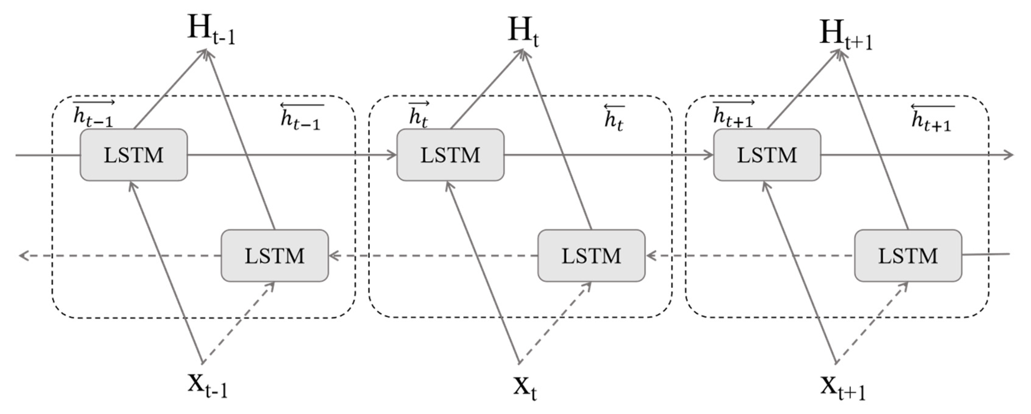
CEEMDAN offers an enhanced decomposition compared to EMD and EEMD, specifically targeting the mode-mixing problem [14]. Its key feature is the adaptive addition of Gaussian noise followed by ensemble averaging. This process effectively cancels out the noise while improving the separation of intrinsic mode functions. The realization steps are as follows:

Gaussian white noise is added to the original PV plant irradiance signal y(t):

$$y_i\left(t\right)=y\left(t\right)+\epsilon {\omega }_i\left(t\right)$$

(5)

where $\epsilon$ is the white noise weighting factor; ${\omega }_i\left(t\right)$ is the white noise added at the ith time’s processing.

The irradiance signal $y_i(t)$ after the addition of white noise was decomposed using the EMD method to obtain the first modal component ${IMF}_1$ and the residuals $r_1\left(t\right)$.

$${IMF}_1(t)={\displaystyle \frac{1}{K}}\sum _{i=1}^K{IMF}_{i1}\left(t\right)$$

(6)

$$r_1\left(t\right)=y\left(t\right)-{IMF}_1\left(t\right)$$

(7)

where $K$ is the number of times white noise is added.

White noise is added to the residuals $r_1\left(t\right)$, and then EMD decomposition is performed to obtain the second modal component ${IMF}_2$ and $r_2\left(t\right)$.

$${IMF}_1(t)={\displaystyle \frac{1}{K}}\sum _{i=1}^K\left(E_1\left(r_1\left(t\right)\right)+{\epsilon }_1{E}_1\left({\omega }_i\right(t\left)\right)\right)$$

(8)

$$r_2\left(t\right)=r_1\left(t\right)-{IMF}_1\left(t\right)$$

(9)

where E is the EMD.

Repeat the above steps and stop when the residuals can no longer be decomposed. The final decomposition of the raw irradiance signal is as follows:

$$y(t)=\sum _{n=1}^K{IMF}_n+R\left(t\right)$$

(10)

2.3. BiLSTM

The bidirectional long short-term memory network [20], an extension of the bidirectional recurrent neural network, enhances learning by incorporating future information. This addresses the limitations of unidirectional LSTMs, which may not fully capture the temporal dependencies within data. Unlike unidirectional LSTMs, BiLSTMs employ two independent LSTM layers to process the input sequence in both forward and backward directions. This dual-directional approach enables the model to learn from both past and future contexts, improving the model’s ability to capture dependencies and ultimately enhancing prediction accuracy. The hidden layer of a BiLSTM comprises forward and backward components, the structure diagram is shown in Figure 2, mathematically represented as follows:

$${\overrightarrow{h}}_t={\lambda }_{\overrightarrow{LSTM}}(h_{t-1},x_t,c_{t-1})$$

(11)

$${\overleftarrow{h}}_t={\lambda }_{\overleftarrow{LSTM}}(h_{t+1},x_t,c_{t+1})$$

(12)

$$H_t=\left[{\overrightarrow{h}}_t,{\overleftarrow{h}}_t\right]$$

(13)

where ${\overrightarrow{h}}_t$, ${\overleftarrow{h}}_t$ are outputs of forward and reverse LSTM layers at time step; $H_t$ represents the outputs of BiLSTM at the time step.

2.4. Information Extractor Model

The conventional self-attention mechanism, by assigning weights to all input information, risks incorporating irrelevant data that can negatively impact output accuracy. To mitigate prediction inaccuracies with long input sequences, Informer prioritizes salient features reflecting key characteristics. This approach effectively reduces the temporal dimension of the input, enabling the extraction of more crucial historical information [21,22,23].

The Informer model, as depicted in Figure 3, adopts an encoder–decoder structure. The encoder incorporates ProbSparse self-attention, a computationally efficient mechanism replacing traditional self-attention, alongside a self-attention distilling procedure for dimensionality reduction. The decoder employs a generative approach, directly producing all predictions in parallel, thus expediting the inference process [13].

The Informer model, as depicted in Figure 3, adopts an encoder–decoder structure. The encoder incorporates ProbSparse self-attention, a computationally efficient mechanism replacing traditional self-attention, alongside a self-attention distilling procedure for dimensionality reduction. The decoder employs a generative approach, directly producing all predictions in parallel, thus expediting the inference process:

$$A(Q,K,V)=Soft\mathit{max}(Q{K}^{\mathsf{{\rm T}}}/\sqrt{d})V$$

(14)

where $Q\in R^{L_Q\times d},K\in R^{L_K\times d},V\in R^{L_V\times d}$, and $d$ are the input dimensions.

In addition, Informer uses the distilling method to assign higher weights to dominant features with primary information and generates a focused self-attention feature map for the previous layer at the j + 1 layer, as shown in Equation (4):

$$X_{j+1}^t=MaxPooling\left(ELU{\left(Convld\right(X_j^t)}_{att}\right))$$

(15)

${(·)}_{att}$ represents the attention module; $X_j^t$ represents the first $j$ layer matrix; $Convld(·)$ denotes a one-dimensional convolution operation on the time series, and exponential linear units (ELUs) are used as the activation function, and finally, the computation of each layer is halved by a Max Pooling layer with a step size of 2, so that the model can retain the information of the long input time series.

For the decoder, the input time series $X_{feed\_de}^t$ is divided into two parts, the known sequence before the point being predicted $X_{token}^t$ and the predicted sequence that needs to be masked from future weather data $X_0^t$:

$$X_{feed\_de}^t=Concat(X_{token}^t,X_0^t)\in R^{(L_{token}+L_y)\propto d_{model}}$$

(16)

In the formula, $L_{token}$, $L_y$ are the lengths of known and predicted sequences, respectively; $d_{model}$ denotes the dimension of the model; $Concat(·)$ denotes the splicing operation.

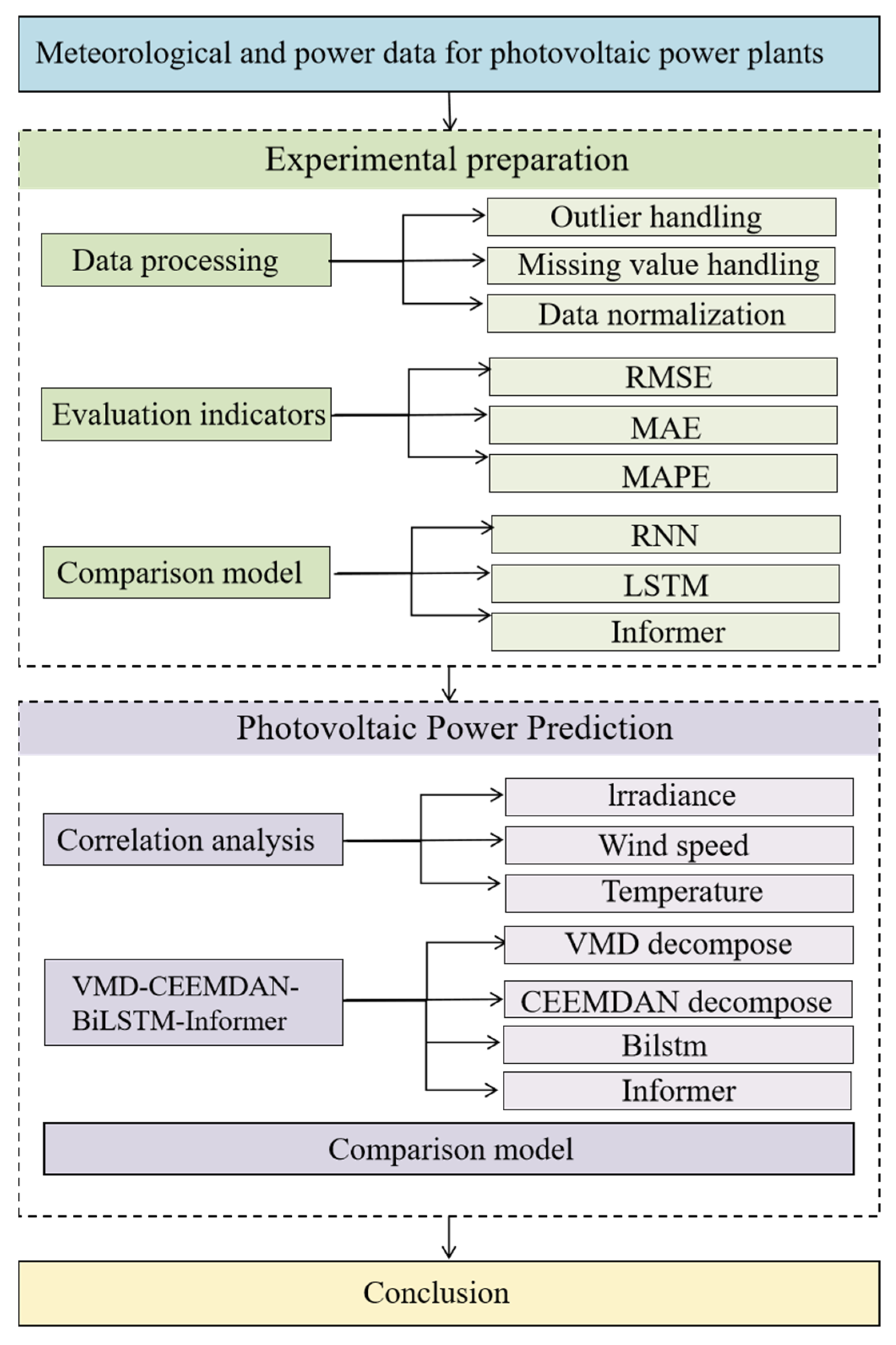
3. Modeling of Ultra-Short-Term PV Power Prediction Based on VMD–CEEMDAN–BiLSTM–Informer

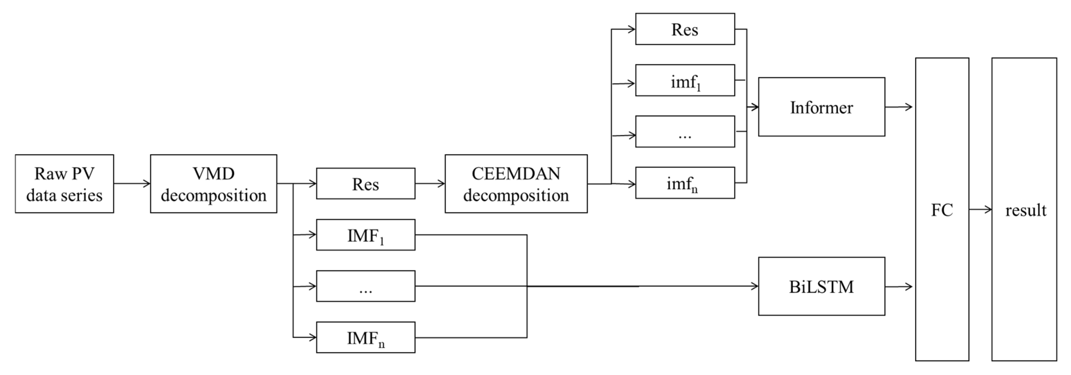
3.1. VMD–CEEMDAN–BiLSTM–Informer Hybrid Model

To address the challenges of non-monotonic and non-smooth raw data in PV power time series prediction, this paper proposes a novel hybrid method, VMD–CEEMDAN–BiLSTM–Informer, for enhanced forecasting accuracy. The approach leverages a secondary decomposition strategy, employing VMD and CEEMDAN, to effectively extract the underlying trends from the complex PV power data, resulting in intrinsic mode functions (IMFs) that capture essential patterns. Subsequently, the BiLSTM network is utilized to capture temporal dependencies within the decomposed data through its inherent recurrent architecture. In parallel, the Informer network, incorporating a sparse attention mechanism and feed-forward network layers, models the data to identify and refine global features efficiently, even within long sequences. The sparse attention mechanism allows for efficient processing of extensive data, while the feedforward network enhances feature integration, leading to a more comprehensive understanding of global data patterns. The parallel architecture of VMD-CEEMDAN, BiLSTM, and Informer allows for comprehensive feature extraction and modeling. The specific modeling steps are detailed in Figure 4.

(1)

Primary decomposition: The collected PV data are preprocessed. Firstly, the number of VMD layers is determined by the center frequency, and then the PV data are decomposed to obtain several $\mathrm{I}\mathrm{M}\mathrm{F}$ component sequences and residuals with lower complexity and nonlinearity.

(2)

Secondary decomposition: The residual components obtained in the previous step are further decomposed using CEEMDAN to obtain the subsequence imf and the smooth residual term, and all the sequences are used as inputs to the prediction model.

(3)

The BiLSTM model, which captures short-term time-dependent and local features in parallel prediction, is used to model the temporal information of the IMF of the VMD, while the Informer model, which can efficiently capture global trends, is used to predict the imf components obtained from the secondary decomposition of the CEEMDAN, and the features of each decomposed signal are extracted.

(4)

Finally, the feature output of each decomposed signal is reconstructed and superimposed through the fully connected layer (FC) to obtain the final power prediction result.

3.2. Assessment Indicators

In this paper, the root mean square error (RMSE) and the mean absolute error (MAE) are used to carry out the description of the results of prediction. The following are the specific formulas:

$$RMSE=\sqrt{{\displaystyle \frac{1}{n}}\sum _{i=1}^n{\left({\widehat{y}}_i-y_i\right)}^2}$$

(17)

$$MAE={\displaystyle \frac{1}{n}}\sum _{i=1}^n\left|{\widehat{y}}_i-y_i\right|$$

(18)

$$R^2=1-{\displaystyle \frac{{\sum }_{i=1}^n{(y_i-\widehat{y_i})}^2}{{\sum }_{i=1}^n{(y_i-\overline{y_i})}^2}}$$

(19)

where n denotes the amount of data in the time series, ${\widehat{y}}_i$ denotes the predicted value, and y_i denotes the actual value.

The RMSE can reflect the accuracy of the prediction results, but it is easily affected by the extreme values. The MAE indicates the absolute mean of all the error values in the sequence.

4. Experimental Contents

4.1. Dataset

This study investigates the performance of a distributed photovoltaic (PV) power plant supplying electricity to a small Australian village, using one year of historical generation data (1 January 2017 to 31 December 2017) [25]. The model’s performance was validated using data from multiple sites within the PV plant. Specifically, data from one site, recorded at 5 min intervals (288 data points per day, totaling 105,120 points), were divided into training and testing sets with an 8:2 ratio. The dataset contained a minimal amount of missing data (0.018%).

For the missing data caused by the actual operation of PV power plants, a small number of missing datasets are replaced using linear interpolation [26], and a large number of missing datasets are replaced using data corresponding to the same data points from the previous day. For the extracted data, use normalization, as in Equation (20):

$$x^{\prime }={\displaystyle \frac{x-\mathit{min}\left(x\right)}{\mathit{max}\left(x\right)-\mathit{min}\left(x\right)}}$$

(20)

where x′ denotes the normalized data value, and x denotes the un-normalized data value. max(x) and min(x) denote the maximum and minimum values in the sequence, respectively.

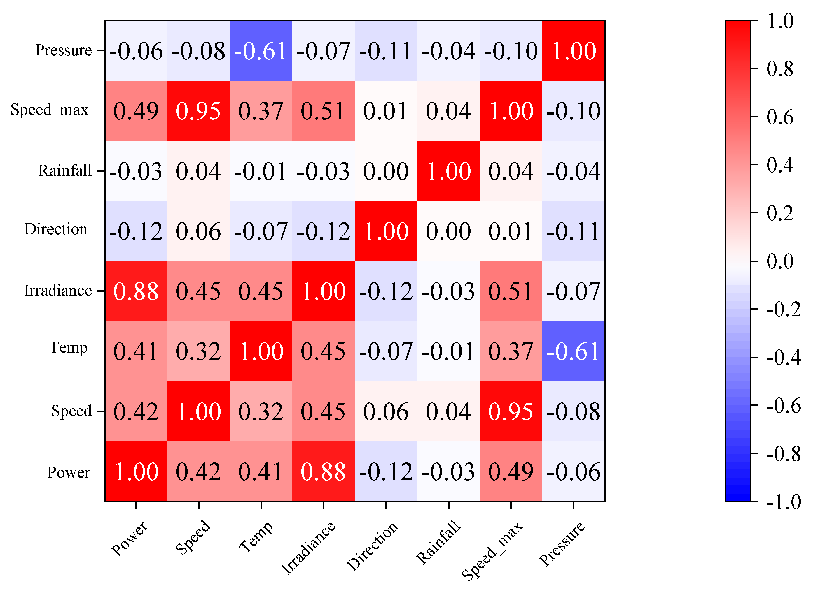
4.2. PV-Output-Influencing Factors and Clustering

The Pearson correlation coefficient is a measure of the correlation (linear correlation) between two variables, X and Y, with a value between −1 and 1 [27]. The formula is as follows:

$$r={\displaystyle \frac{{\sum }_{i=1}^n(X_i-\overline{X})(Y_i-\overline{Y})}{\sqrt{{\sum }_{i=1}^n(X_i-\overline{X}{)}^2}\sqrt{{\sum }_{i=1}^n(Y_i-\overline{Y}{)}^2}}}$$

(21)

Pearson’s correlation coefficient analyses were performed on the data available from the PV site. The thermodynamic diagram of correlation coefficient is shown in Figure 5

Irradiance exhibits the strongest positive correlation with actual power output ($r$ = 0.88), followed by maximum wind speed ($r$ = 0.49). Wind direction shows the highest negative correlation ($r$ = −0.12), while barometric pressure displays a weaker negative correlation ($r$ = −0.063). Consequently, irradiance, air temperature, and wind speed were selected as input variables for the model.

Clustering of seasonally segmented historical data identified three typical PV generation profiles associated with sunny, cloudy, and rainy days, as illustrated in Figure 6.

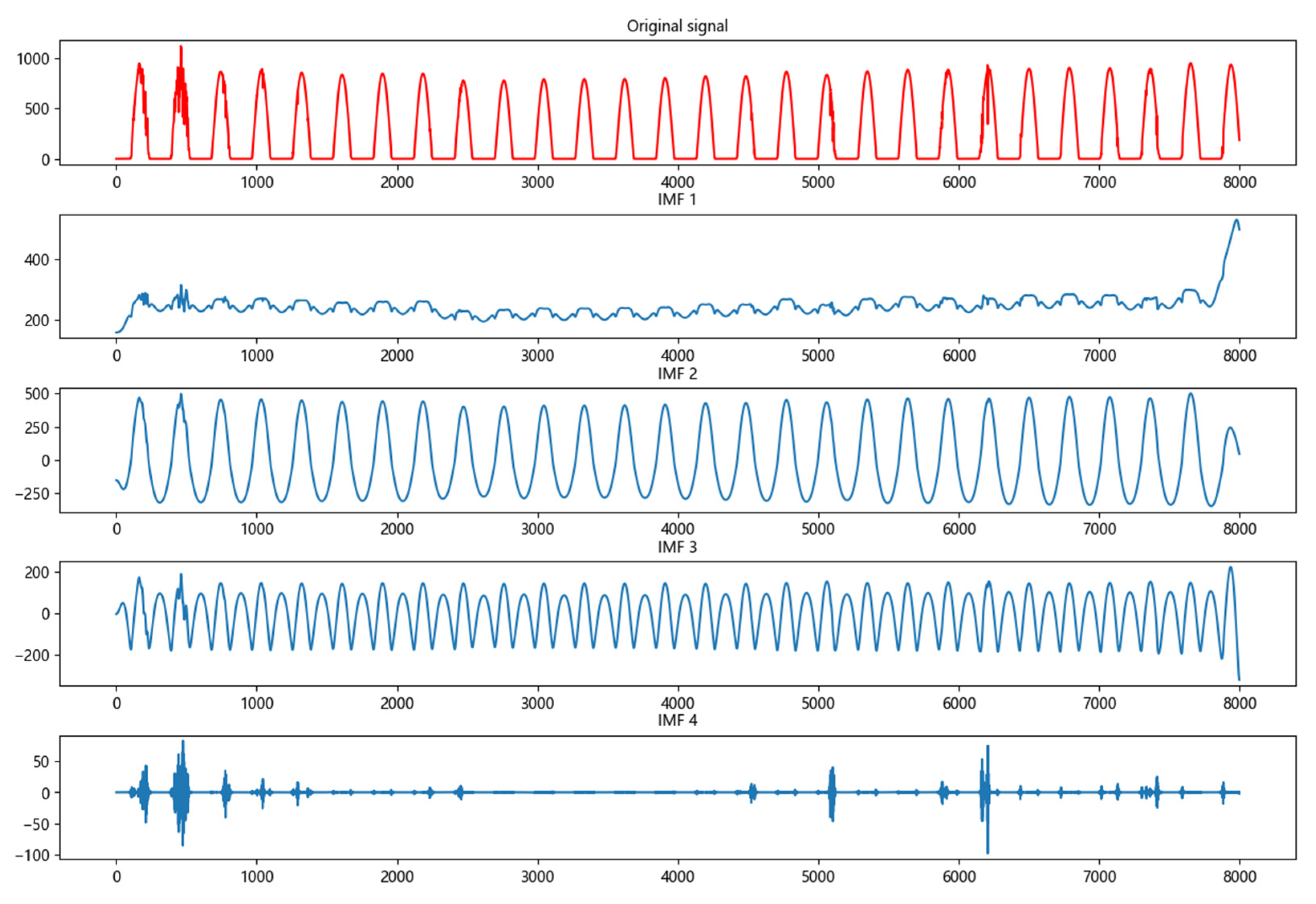
4.3. Secondary Decomposition

The residual terms underwent EMD, as illustrated in Figure 7. EMD yielded ten IMFs and one RES. The decomposition process progressively increased the period of vibration and reduced the fluctuation of each component relative to the original residual, effectively enhancing smoothness. This simplification of the data, while preserving essential information, facilitates prediction model training and subsequently improves forecast accuracy.

As the PV power output time series data are regularly fluctuating and noisy, firstly, the original sequence of irradiance is decomposed by using the penalty factor and the convergence stop condition; in order to avoid the phenomenon of insufficient decomposition or over-decomposition of irradiance sequence, the value is determined by the method of observing the ratio of the center frequency, respectively, so that $\mathrm{K}=\mathrm{3,4},\mathrm{5,6},\mathrm{7,8}$. With K = 5, the calculated maximum center frequency reaches 0.266161. However, to mitigate over-decomposition, K was set to 4. The resulting components, illustrated in Figure 7, exhibit distinct center frequencies, effectively reducing signal volatility and simplifying feature mapping for PV power time series analysis.

To further refine the residual component obtained from VMD, CEEMDAN is applied. The CEEMDAN parameters are configured as follows: trials = 200, epsilon = 0.2; remaining parameters are set to their default values. The resulting components, as illustrated in Figure 8, exhibit a progressive increase in vibration period and a decrease in fluctuation amplitude following each residual decomposition. This process effectively enhances the smoothness of the data compared to the original signal. By reducing data complexity and improving smoothness while preserving essential information, this pre-processing step facilitates improved learning by the prediction model and enhances subsequent prediction accuracy.

To evaluate the effectiveness of the proposed secondary decomposition method,

Table 1. Comparison of prediction errors of various decomposition methods.

Seasonal Type	Decomposition Methods	MAE	RMSE	R2
Sunny day	VMD	0.212	0.258	0.9586
	CEEMDAN	0.175	0.230	0.9687
	Secondary decomposition	0.084	0.108	0.989
Cloudy day	VMD	0.217	0.282	0.921
	CEEMDAN	0.218	0.277	0.934
	Secondary decomposition	0.084	0.150	0.979
Rainy day	VMD	0.275	0.372	0.856
	CEEMDAN	0.264	0.361	0.879
	Secondary decomposition	0.130	0.208	0.966

presents the PV power prediction errors achieved by applying VMD, CEEMDAN, and the secondary decomposition method to BiLSTM–Informer models using data from sunny, cloudy, and rainy days.

All decomposition methods exhibited lower prediction errors for sunny days compared to cloudy and rainy days. Notably, the secondary decomposition method yielded the smallest prediction errors and highest accuracy for categorical data compared to VMD and CEEMDAN.

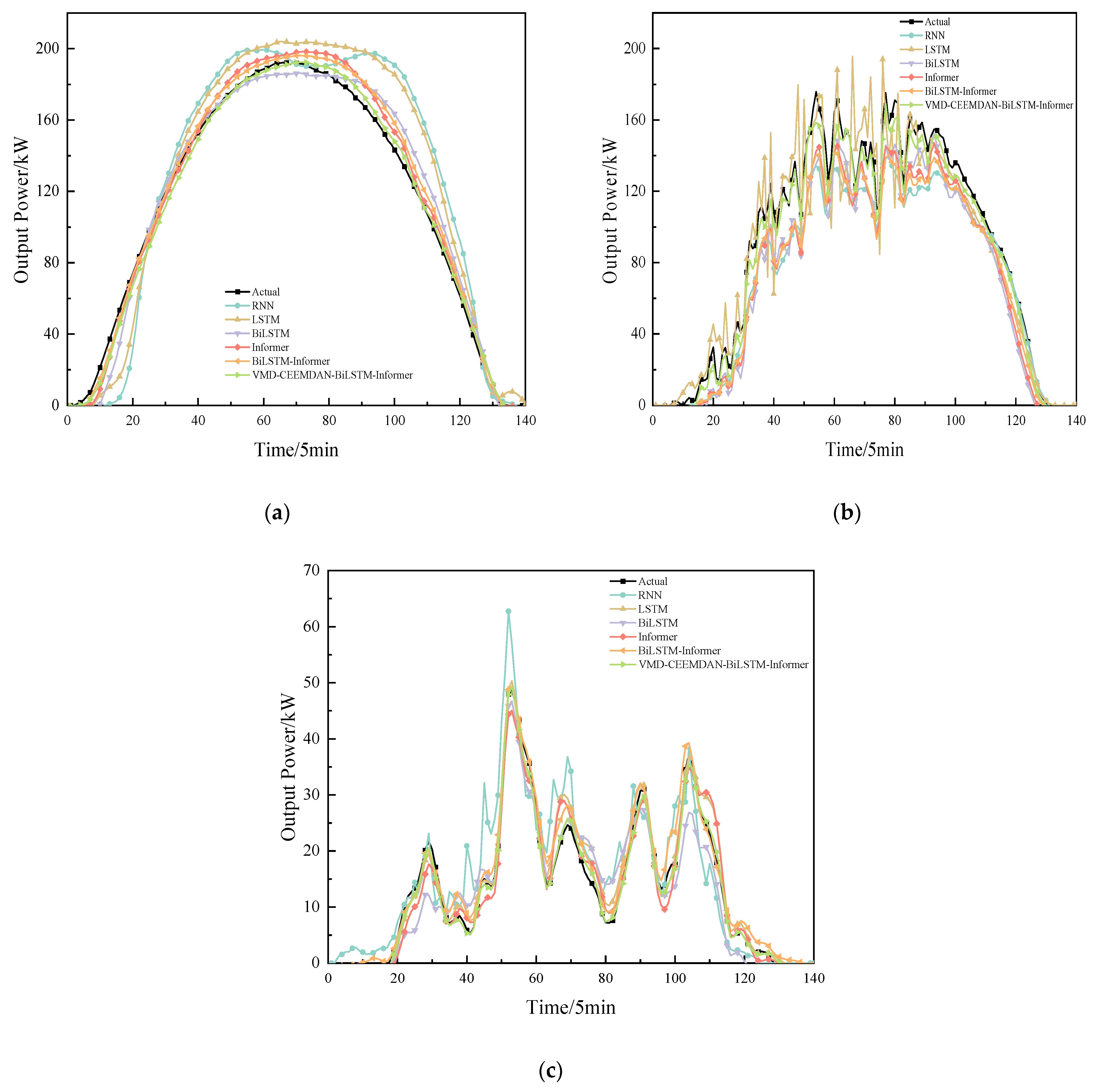
4.4. VMD–CEEMDAN–BiLSTM–Informer Power Prediction

The IMF from the VMD is fed into BiLSTM, setting BiLSTM’s Hidden Dim = 128, Layers = 2, Dropout = 0.3, Batch Size = 64, Learning Rate = 1 × 10⁻³, and the IMF produced by the secondary decomposition is fed into Informer, setting Informer’s Hidden Dim = 256, Layers = 4, Attention Heads = 8, Dropout = 0.3, Batch Size = 32, Learning Rate = 1 × 10⁻⁴. The networks designed in this paper use an Adam optimizer, with the epoch set to 1000 (epoch represents the number of training rounds) and the loss function is L1 loss. The model of this paper was compared with other models, and the results are shown in the

Table 2. Comparison of prediction errors for various meteorological days under different models.

Seasonal Type	Model	RMSE	MAE	R2
Sunny day	RNN	0.3339	0.2067	0.8975
	LSTM	0.2595	0.1781	0.9255
	BiLSTM	0.2004	0.1262	0.9555
	Informer	0.1870	0.1201	0.9613
	BiLSTM–Informer	0.1161	0.0984	0.9865
	VMD–CEEMDAN–BiLSTM–Informer	0.1082	0.0842	0.9894
Cloudy day	RNN	0.2903	0.1930	0.9164
	LSTM	0.2729	0.1986	0.9261
	BiLSTM	0.2628	0.2029	0.9315
	Informer	0.1914	0.1036	0.9636
	BiLSTM–Informer	0.1688	0.1027	0.9717
	VMD–CEEMDAN–BiLSTM–Informer	0.1504	0.0849	0.9794
Rainy day	RNN	0.4017	0.2585	0.8412
	LSTM	0.3689	0.2186	0.8754
	BiLSTM	0.3407	0.1874	0.9038
	Informer	0.3013	0.1654	0.9247
	BiLSTM–Informer	0.2260	0.1480	0.9606
	VMD–CEEMDAN–BiLSTM–Informer	0.2085	0.1309	0.9664

.

To visually assess the impact of optimization, a representative day for each weather type was randomly selected. The predicted power curve of the combined model was then compared to the actual power curve, allowing for a clear evaluation of performance improvements across diverse weather conditions (Figure 9).

Under sunny conditions, PV output exhibits low volatility, leading to accurate predictions across most models. However, RNN, LSTM, and BiLSTM models show comparatively weaker performance. Conversely, cloudy and rainy days induce greater power output fluctuations, resulting in poorer predictions for RNN, LSTM, and BiLSTM. The VMD–CEEMDAN–BiLSTM–Informer model demonstrates superior predictive capability under these variable weather conditions, closely aligning with actual power measurements. Comparative analysis of prediction curves confirms the VMD–CEEMDAN–BiLSTM–Informer model’s closer approximation to the observed power output, indicating its overall superior performance among the evaluated models.

Under the three weather conditions examined, the VMD–CEEMDAN–BiLSTM–Informer model demonstrated superior performance compared to BiLSTM–Informer and Informer models. Specifically, the VMD–CEEMDAN–BiLSTM–Informer model exhibited lower RMSE, MAE, and R² values. Compared to the second-best-performing BiLSTM–Informer model, the proposed model achieved RMSE reductions of 6.80%, 10.91%, and 7.74% and MAE reductions of 14.41%, 17.33%, and 11.55% for sunny, cloudy, and overcast days, respectively. These results indicate that the secondary decomposition strategy enhances the prediction accuracy of the BiLSTM–Informer architecture. Furthermore, in comparison to RNN, the VMD–CEEMDAN–BiLSTM–Informer model yielded substantial improvements, with RMSE reductions of 67.59%, 48.19%, and 48.09% and MAE reductions of 59.26%, 56.01%, and 49.36% for sunny, cloudy, and overcast days, respectively. This demonstrates the superior predictive capability of the proposed VMD–CEEMDAN–BiLSTM–Informer model relative to all other models evaluated.

The analysis of data across varying weather conditions demonstrates the effectiveness of the VMD–CEEMDAN–BiLSTM–Informer model in enhancing the accuracy of photovoltaic power forecasting.

5. Conclusions

(1)

Key meteorological factors influencing PV power generation were identified through data processing and analysis. The data were then categorized into sunny, cloudy, and rainy days using clustering, enabling the development of weather-specific predictive models.

(2)

Employing VMD and CEEMDAN for secondary data decomposition effectively mitigates modal aliasing while preserving the inherent characteristics of the PV sequence. This approach yields multiple intrinsic mode functions (IMFs) with varying temporal scales, thereby capturing the localized dynamics of PV power generation and minimizing the influence of sequence complexity on prediction accuracy.

(3)

The proposed BiLSTM–Informer architecture leverages the strengths of both models. BiLSTM effectively models bidirectional error patterns, and Informer’s attention efficiently identifies crucial temporal relationships within the feature set, leading to improved prediction performance.

This paper introduces a secondary decomposition method that, compared to single-decomposition techniques, enhances the extraction of temporal information from time series data. This approach mitigates data instability and improves prediction accuracy. Empirical results demonstrate that the proposed model achieves a reduction in prediction error and exhibits superior accuracy compared to conventional forecasting models. While the model demonstrates improved performance in photovoltaic (PV) power prediction under cloudy and rainy conditions, the inherent variability of irradiance during these weather patterns presents a persistent challenge. Future research should focus on refining weather classification to further enhance prediction accuracy across a wider range of meteorological conditions.

References

1. Duda, J.; Kusa, R.; Pietruszko, S.; Smol, M.; Suder, M.; Teneta, J.; Wójtowicz, T.; Żdanowicz, T. Development of Roadmap for Photovoltaic Solar Technologies and Market in Poland. Energies 2022, 15, 174. [Google Scholar] [CrossRef]
2. Yang, X.; Xu, C.; Zhang, Y.; Yao, W.; Wen, J.; Cheng, S. Real-Time Coordinated Scheduling for ADNs with Soft Open Points and Charging Stations. IEEE Trans. Power Syst. 2021, 36, 5486–5499. [Google Scholar] [CrossRef]
3. Kundur, P. Sustainable Electric Power Systems in the 21st Century: Requirements, Challenges and the Role of New Technologies. In Proceedings of the IEEE Power Engineering Society General Meeting, Denver, CO, USA, 6–10 June 2004; Volume 2, pp. 2297–2298. [Google Scholar]
4. Yang, X.; Zhang, Y.; He, H.; Ren, S.; Weng, G. Real-Time Demand Side Management for a Microgrid Considering Uncertainties. IEEE Trans. Smart Grid 2019, 10, 3401–3414. [Google Scholar] [CrossRef]
5. Qin, Y.; Xu, Y.; Wang, X.; Wang, T.; Li, W. Study on Short-Term Photovoltaic Output Prediction Based on Improved FCM-LSTM. Acta Energiae Solaris Sin. 2024, 45, 304. [Google Scholar] [CrossRef]
6. Cui, Y.; Sun, Y.C.; Chang, Z.L. A Review of Short-Term Solar Photovoltaic Power Generation Prediction Methods. Resour. Sci. 2013, 35, 1474–1481. [Google Scholar]
7. Pretto, S.; Ogliari, E.; Niccolai, A.; Nespoli, A. A New Probabilistic Ensemble Method for an Enhanced Day-Ahead PV Power Forecast. IEEE J. Photovolt. 2022, 12, 581–588. [Google Scholar] [CrossRef]
8. Zhao, B.; Wang, Y.; Wang, B.; Xuan, W.; Lei, Z.; Ge, L.; Xv, X. Research on the output power prediction method of distributed photovoltaic systems based on ARIMA time series. Renew. Energy 2019, 37, 820–823. [Google Scholar]
9. Hou, W.; Xiao, J.; Niu, L. A prediction method for photovoltaic power generation system output based on grey theory. Electr. Technol. 2016, 53–58. [Google Scholar] [CrossRef]
10. Li, Y.; Huang, W.; Lou, K.; Zhang, X.; Wan, Q. Short-Term PV Power Prediction Based on Meteorological Similarity Days and SSA-BiLSTM. Syst. Soft Comput. 2024, 6, 200084. [Google Scholar] [CrossRef]
11. Yang, M.; Han, C.; Zhang, W.; Wang, B. A Short-Term Power Prediction Method for Wind Farm Cluster Based on the Fusion of Multi-Source Spatiotemporal Feature Information. Energy 2024, 294, 130770. [Google Scholar] [CrossRef]
12. Yang, M.; Huang, Y.; Guo, Y.; Zhang, W.; Wang, B. Ultra-Short-Term Wind Farm Cluster Power Prediction Based on FC-GCN and Trend-Aware Switching Mechanism. Energy 2024, 290, 130238. [Google Scholar] [CrossRef]
13. Zhou, H.; Zhang, S.; Peng, J.; Zhang, S.; Li, J.; Xiong, H.; Zhang, W. Informer: Beyond Efficient Transformer for Long Sequence Time-Series Forecasting. Proc. AAAI Conf. Artif. Intell. 2021, 35, 11106–11115. [Google Scholar] [CrossRef]
14. Tan, H.; Yang, Q.; Xing, J. Photovoltaic Power Prediction Based on Combined Xgboost-Lstm Model. Acta Energiae Solaris Sin. 2022, 43, 75. [Google Scholar] [CrossRef]
15. Jaihuni, M.; Basak, J.K.; Khan, F.; Okyere, F.G.; Sihalath, T.; Bhujel, A.; Park, J.; Lee, D.H.; Kim, H.T. A Novel Recurrent Neural Network Approach in Forecasting Short Term Solar Irradiance. ISA Trans. 2022, 121, 63–74. [Google Scholar] [CrossRef]
16. Zhang, Y.; Cheng, Q.; Jiang, W.; Liu, X.; Shen, L.; Chen, Z.H. A photovoltaic power prediction model based on EMD-PCA-LSTM. Acta Energiae Solaris Sinica 2021, 42, 62–69. [Google Scholar]
17. Dong, X.; Zhao, H.; Zhao, S.; Lu, D.; Chen, X.; Liu, L. Ultra-short-term photovoltaic power prediction based on SOM clustering and secondary decomposition of BiGRU. Acta Energiae Solaris Sinica 2022, 43, 85–93. [Google Scholar] [CrossRef]
18. Sharma, V.; Parey, A. Extraction of Weak Fault Transients Using Variational Mode Decomposition for Fault Diagnosis of Gearbox under Varying Speed. Eng. Fail. Anal. 2020, 107, 104204. [Google Scholar] [CrossRef]
19. Dragomiretskiy, K.; Zosso, D. Variational Mode Decomposition. IEEE Trans. Signal Process. 2014, 62, 531–544. [Google Scholar] [CrossRef]
20. Hochreiter, S.; Schmidhuber, J. Long Short-Term Memory. Neural Comput. 1997, 9, 1735–1780. [Google Scholar] [CrossRef]
21. Shi, Z.; Li, J.; Jiang, Z.; Li, H.; Yu, C.; Mi, X. WGformer: A Weibull-Gaussian Informer Based Model for Wind Speed Prediction. Eng. Appl. Artif. Intell. 2024, 131, 107891. [Google Scholar] [CrossRef]
22. Peng, T.; Fu, Y.; Wang, Y.; Xiong, J.; Suo, L.; Nazir, M.S.; Zhang, C. An Intelligent Hybrid Approach for Photovoltaic Power Forecasting Using Enhanced Chaos Game Optimization Algorithm and Locality Sensitive Hashing Based Informer Model. J. Build. Eng. 2023, 78, 107635. [Google Scholar] [CrossRef]
23. Cao, Y.; Liu, G.; Luo, D.; Bavirisetti, D.P.; Xiao, G. Multi-Timescale Photovoltaic Power Forecasting Using an Improved Stacking Ensemble Algorithm Based LSTM-Informer Model. Energy 2023, 283, 128669. [Google Scholar] [CrossRef]
24. Xu, X.; Guan, L.; Wang, Z.; Yao, R.; Guan, X. A Double-Layer Forecasting Model for PV Power Forecasting Based on GRU-Informer-SVR and Blending Ensemble Learning Framework. Appl. Soft Comput. 2025, 172, 112768. [Google Scholar] [CrossRef]
25. Desert Knowledge Australia Centre. 01/01/2017. Download Data. Australia’s iconic Uluru (Ayers Rock). Available online: http://dkasolarcentre.com.au/historical-data/download (accessed on 24 December 2024).
26. Mellit, A.; Kalogirou, S.A. Artificial Intelligence Techniques for Photovoltaic Applications: A Review. Prog. Energy Combust. Sci. 2008, 34, 574–632. [Google Scholar] [CrossRef]
27. Jiang, Y.; Fu, K.; Huang, W.; Zhang, J.; Li, X.; Liu, S. Ultra-Short-Term PV Power Prediction Based on Informer with Multi-Head Probability Sparse Self-Attentiveness Mechanism. Front. Energy Res. 2023, 11, 1301828. [Google Scholar] [CrossRef]
Figure 1. Flowchart of short-term PV power prediction based on VMD–CEEMDAN–BiLSTM–Informer model.
Energies 18 01485 g001
Figure 2. Structure of bi-directional long short-term memory network (BiLSTM).
Energies 18 01485 g002
Figure 3. Structure of Informer model [24].
Energies 18 01485 g003
Figure 4. Structure of EMD-BiLSTM–Informer.
Energies 18 01485 g004
Figure 5. Correlation between PV power and factors.
Energies 18 01485 g005
Figure 6. Classification of three typical weather clusters for four seasons.
Energies 18 01485 g006
Figure 7. VMD results.
Energies 18 01485 g007
Figure 8. CEEMDAN decomposition results.
Energies 18 01485 g008
Figure 9. Comparison of model prediction results under different weather conditions: (a) sunny day; (b) cloudy day; (c) rainy day.
Energies 18 01485 g009