State-of-Health Estimation of Lithium-Ion Batteries Based on Electrochemical Impedance Spectroscopy Features and Fusion Interpretable Deep Learning Framework

Abstract

Monitoring and accurately predicting the state of health (SOH) of lithium-ion batteries (LIBs) is essential for ensuring safety, particularly in detecting early signs of potential failures such as overheating and incorrect charging and discharging practices. This paper introduces a network architecture called CGMA-Net (Convolutional Gated Multi-Attention Network), which is designed to effectively address the issue of battery capacity degradation. The network architecture performs initial feature extraction and filtering through convolutional layers, extracting potential key features from the raw input data. The multi-head attention mechanism is the core of this framework, enabling the model to perform weighted analysis of input features. This enables the model to provide a more transparent decision-making process, assisting in the discovery and interpretation of key features within battery SOH estimation. Moreover, a GRU (gated recurrent unit) architecture is introduced in the intermediate layers of the model to ensure its generalization ability, further improving overall prediction performance. A multiple cross-validation approach is adopted to ensure the model’s adaptability across different battery samples, enabling flexible estimation of battery SOH. The experimental results show that the average RMSE (Root Mean Squared Error) and MAE (Mean Absolute Error) values are within 1 mAh, and the MAPE (Mean Absolute Percentage Error) is below 2.5%.

1. Introduction

Lithium-ion batteries (LIBs), characterized by their high energy density, reliability, and long service life, have been widely applied in portable electronics, electric vehicles, and the storage of electricity derived from renewable sources, underlining their integral role in advancing energy solutions and systems [1,2,3,4]. However, the performance of lithium-ion batteries declines nonlinearly as the usage time increases, not only posing a safety risk for the system but also affecting the continuous application of LIBs. The state of health (SOH) is one of the crucial indicators reflecting the overall condition of the battery. Accurate prediction of SOH helps optimize battery usage and maintenance strategies, thereby extending battery life. This is crucial for LIB applications in electric vehicles and sustainable energy [5].

Battery aging is a complex physicochemical process, influenced by both internal and external factors. The complexity of operational conditions leads to the accumulation of side reaction products within the battery, causing changes in electrochemical equilibrium and rendering the aging process of the battery highly nonlinear [6]. Traditional battery prediction methods primarily rely on the microscopic aging mechanisms of the batteries, such as the decomposition of electrolytes and the loss of active materials [7,8]. Although these methods can offer an in-depth understanding of the battery aging process, the complexity of the battery degradation makes it difficult to characterize and simulate all the mechanisms. Conventional methods for predicting the SOH of LIBs are generally divided into two types, electrochemical models and equivalent circuit models. Electrochemical models are grounded in the physicochemical principles of batteries. In these models, battery performance is predicted by simulating and analyzing the internal electrochemical processes. Commonly used electrochemical models include the Doyle–Fuller–Newman (DFN) model [9] and the single-particle model (SPM) [10]. Equivalent circuit models (ECMs) simulate battery behavior using circuit components such as resistors, capacitors, and inductors. ECMs are generally simpler and more computationally efficient than electrochemical models, making them more suitable for online monitoring and real-time prediction. Common ECMs include the Rint model [11], Thevenin model [12], and PNGV model [13]. Although these methods have obtained acceptable results in predicting the SOH of batteries, they still have certain limitations, such as insufficient understanding of battery aging mechanisms and the challenge of accurately estimating multiple model parameters.

With the advancements of artificial intelligence, data-driven methods have become more and more important in estimating SOH. These techniques predict battery health by analyzing operational data, eliminating the need for directly creating physical models. Support vector machines (SVMs) [14], random forests (RFs) [15], and artificial neural networks (ANNs) [16] are common machine learning approaches. The key advantage of data-driven methods is their ability to process vast amounts of data and adapt to the nonlinear characteristics of battery aging. For example, Qu et al. [17] proposed a hybrid model, combining particle swarm optimization (PSO) and an attention mechanism with the long short-term memory (LSTM) network for monitoring the SOH of LIBs. This model employs incremental learning to update itself dynamically, thereby improving SOH prediction accuracy. Yang et al. [18] presented a technique based on convolutional neural networks (CNNs) for extracting SOH indicators between consecutive charge and discharge cycles, and the random forest algorithm is utilized to generate the final SOH estimation using the indicators from the CNN. Additionally, Sun et al. [19] developed a robust SOH prediction model, utilizing a bidirectional long short-term memory network (BiLSTM) with adaptive weighting strategies. They analyzed health characteristics from lithium-ion battery charge profiles and utilized incremental capacity analysis (ICA) to investigate underlying associations to state of health, identifying peaks within IC curves and associated voltages as additional variables in the model.

With the continuous advancement of deep learning technologies, more methods and complex integrated models have been applied to the SOH estimation of LIBs. For instance, Li et al. [20] introduced a variant long short-term memory neural network (AST-LSTM NN), a modified LSTM neural network, to enhance the forecasting of SOH and remaining useful life (RUL) of LIBs. This novel model incorporates both one-to-one and many-to-one mapping architectures, and is trained for precise SOH and RUL predictions. In another study, Zheng et al. [21] adopted the extreme learning machine methodology to anticipate overall temperature fluctuations during constant current charging by utilizing sporadic and random charging information. By extracting multidimensional health attributes from temperature variation curves to capture the diverse aspects of battery aging, they identified six closely linked features using the Pearson correlation coefficient. Subsequently, a gated recurrent unit (GRU) neural network was implemented for SOH prediction. Yang and team [22] proposed a methodology integrating convolutional neural networks and transfer learning for real-time SOH estimation. The foundational model underwent pre-training with accelerated aging data from various dynamic scenarios, such as over-charging and over-discharging. Through a transfer learning strategy, this base model was fine-tuned with a mere 15% of typical-speed aging data to create a new model, tested on the remaining 85% of the same dataset.

In the field of SOH estimation for LIBs using deep learning methods, feature extraction is a critical step, and the limitations of feature processing can constrain the ability of models. In some studies, SOH estimation methods usually rely on statistical characteristics such as current, voltage, and charge/discharge curves to obtain key parameters. Ref. [23] introduced a method that extracts five relevant features and captures the relationship of capacity on these five features, for estimating the capacity of LIBs based on charging voltage and current curves. Sheng et al. [24] used an online battery capacity estimation method during partial charging cycles by combining voltage, current, and charging capacity data with deep convolutional neural networks (DCNNs). Li et al. [25] utilized signal-to-image transformation and data segmentation techniques to create inputs for CNN models, with the aim of estimating the capacity of LIBs by incorporating partial charging segments and transfer learning. However, the aforementioned studies primarily focus on data processing under stable and specific charging conditions. In fact, batteries show more complexity and dynamism in practical applications, posing challenges to the current feature engineering approaches [26]. For SOH estimation based on EIS features, some studies require manual fitting of impedance data using equivalent circuit models, which may increase the risk of error accumulation and rely on expert experience [27,28,29]. The manual feature engineering process is not only time-consuming but also may lead to inconsistent feature extraction results due to variations in experimental conditions and the experience of operators, further affecting the accuracy of model predictions. The methods for SOH estimation are summarized in

Table 1. Classification of SOH estimation methods.

Input Feature	Model Classification	Specific Methods	Ref.
		DFN	[9]
	Physical model	DP	[11]
		PNGV	[13]
		LSTM-PSO	[17]
		CNN-RF	[18]
Based on charging/ discharging curve		AST-LSTM NN	[20]
	Data-driven	GRU	[21]
		KNN-PSO	[23]
		FRA-CNN	[25]
		ECMC-GPR	[27]
		ECM	[28]
		CAE-DNN	[30]
EIS data		PIDL	[31]
		SSA-Net	[32]
		Transformer	[33]

according to different models and input features.

Furthermore, it is noted that temperature plays essential roles in determining the reliability and safety of LIBs [34]. Different operating temperatures can impact the performance of LIBs to varying degrees, thereby correspondingly shortening their lifespan [35]. Therefore, developing SOH prediction models that can adapt to multi-temperature conditions is crucial for enhancing the adaptability and accuracy of battery management systems. The information of batteries under various temperature conditions can be accurately measured by EIS technology, thus offering an effective feature extraction method for SOH prediction.

In summary, despite significant progress made by data-driven methods in battery SOH prediction, challenges still exist such as the efficiency of feature extraction, the ability of the model to generalize, and the precision of predictions across various temperature conditions. Therefore, this study aims to explore a multi-temperature SOH prediction method based on EIS features and deep learning technologies. The main contributions can be further summarized as follows:

(1)

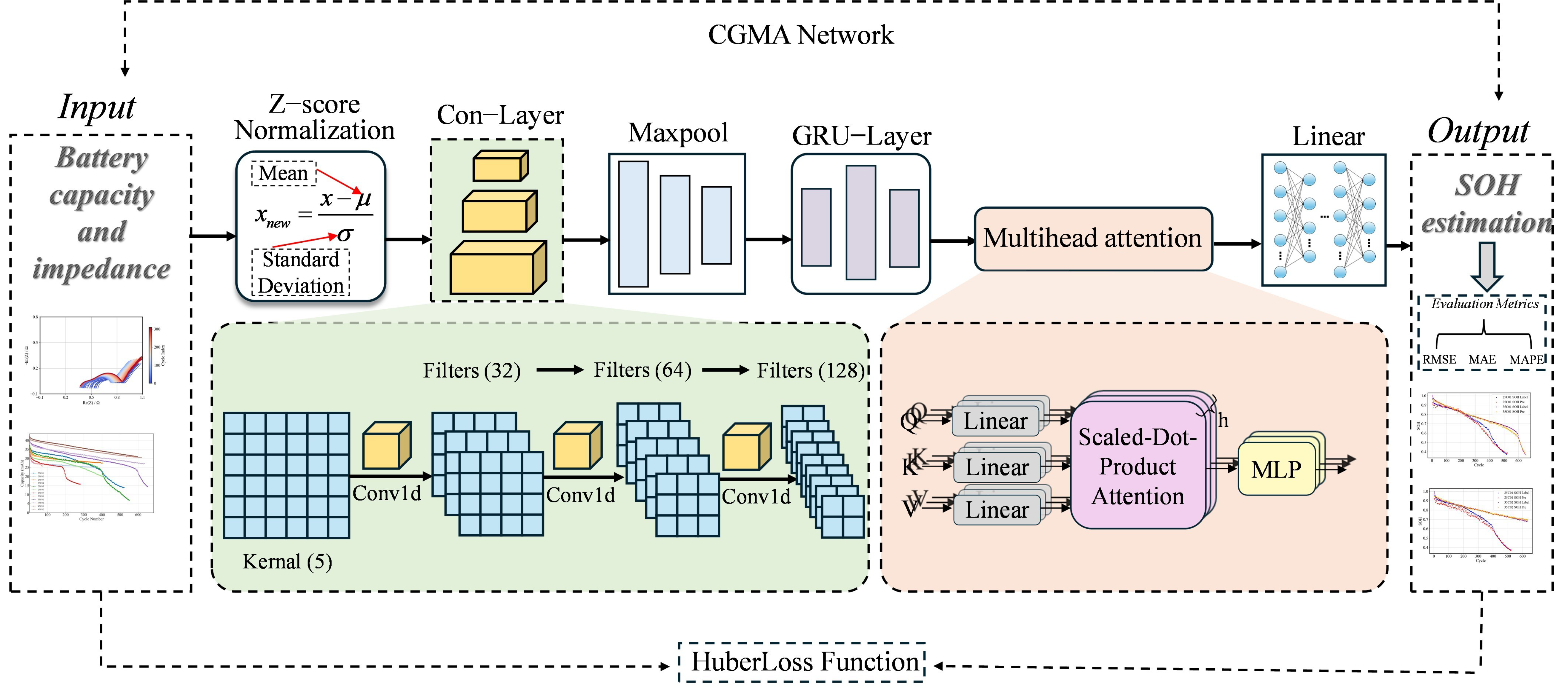
This study proposes a novel deep learning framework called CGMA-Net (Convolutional Gated Multi-Attention Network), which enables flexible estimation of battery SOH under three different temperatures in this dataset.

(2)

In this study, an ensemble model strategy is employed to automatically extract impedance features from multiple modules and track feature variations for information mining. Without the need for complex manual feature engineering, valuable electrochemical information can be extracted from EIS data.

(3)

Comprehensive experiments were conducted to compare the proposed framework with advanced models based on impedance feature–battery SOH estimation research, evaluating its robustness and effectiveness.

The remainder of this paper is organized as follows: Section 2 introduces the battery dataset used in this study and visualizes the impedance data. Section 3 presents the fundamental techniques and framework for SOH prediction of battery based on EIS features. Section 4 discusses the results of battery SOH estimation, including a detailed analysis of the errors and accuracy of the proposed model compared to baseline models. Finally, Section 5 presents the conclusions of this study.

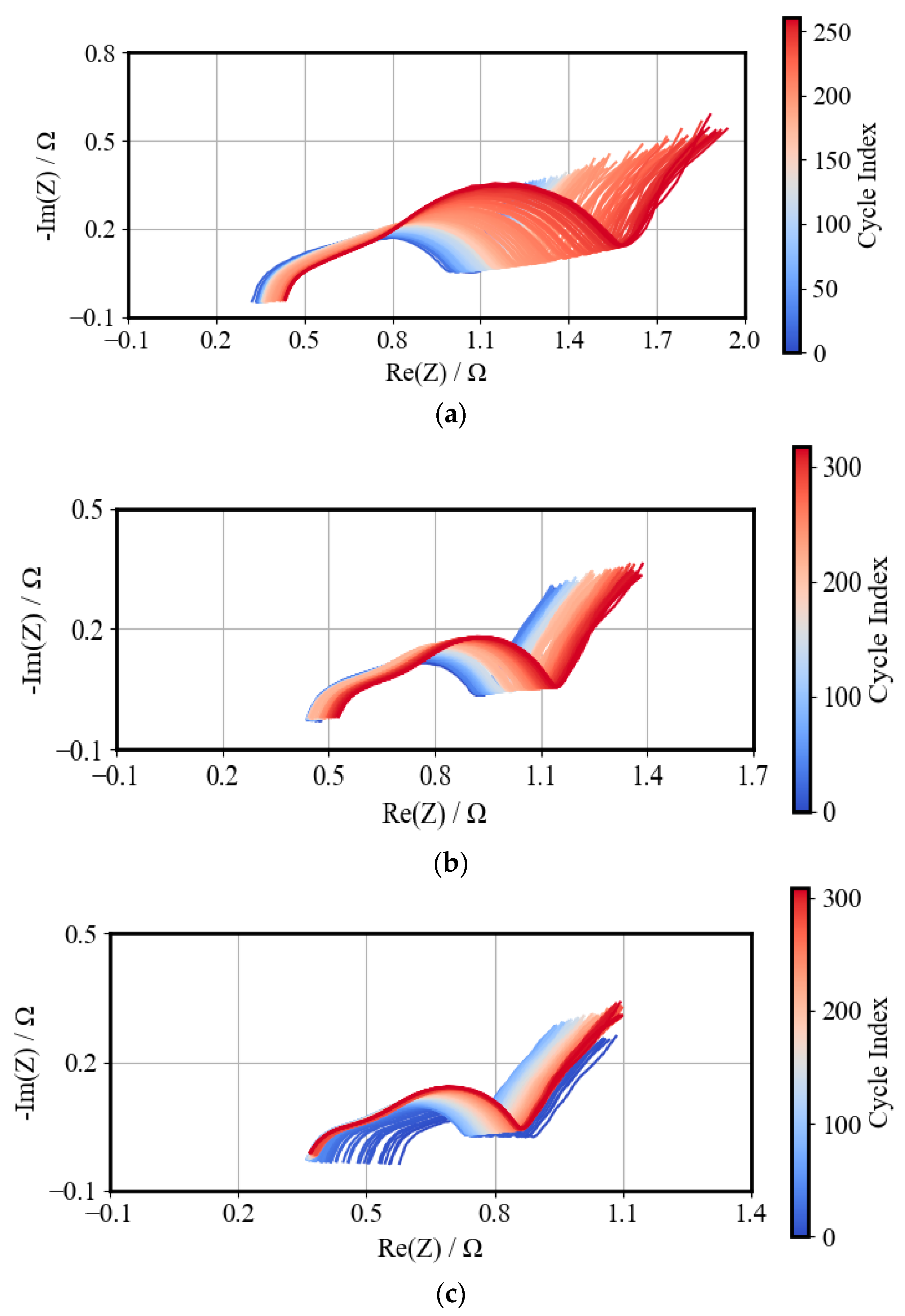
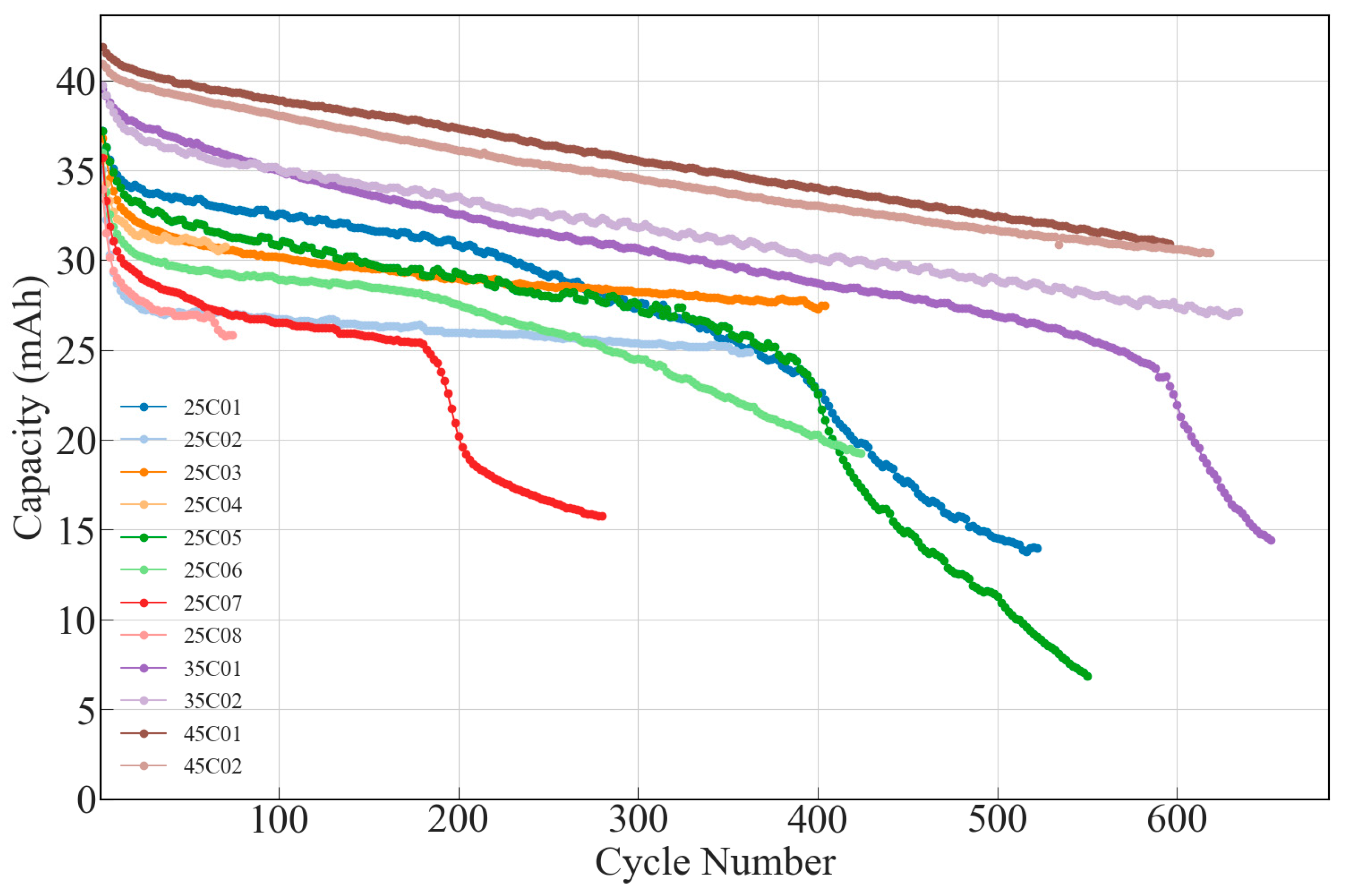
2. Dataset Analysis and Data Pre-Processing

A public dataset available in the Cavendish Laboratory at the University of Cambridge was used in this study. The necessary data were obtained through continuous charge–discharge cycling experiments and electrochemical testing on 12 Eunicell LR2032 Li-ion coin cells with a capacity of 45 mAh [36]. The composition of the cell was graphite/LiCoO₂. The cells underwent testing at three different temperatures. At 25 °C, there were eight test cells (25C01-25C08) with a larger amount of data. At 35 °C and 45 °C, there were four test cells (35C01, 35C02, 45C01, 45C02).

The charging process followed a constant current–constant voltage (CC-CV) strategy at a 1C rate (45 mA) until the voltage reached 4.2 V. The discharge process was carried out at a 2C rate (90 mA) through constant current (CC) discharge until the voltage decreased to 3.0 V. Throughout the charging and discharging operations of the cell, EIS data were gathered in nine distinct conditions (I~IX). States I to IX represented the measured states during the three processes of battery resting, charging, and discharging. State V and IX represented the impedance data measured after the battery had rested for 15 min following charging and discharging, respectively. The other states corresponded to the EIS data monitored during the charging and discharging processes. After the battery rested, its electrochemical state became relatively stable. The EIS data measured at State V was used as the model input in this study. The excitation current was 5 mA, with a frequency range of 0.02 Hz–20 kHz.

To better understand the data in the dataset, part of the data was selected for visualization, laying the foundation for the input of subsequent models. Among them, Figure 1 shows the trend chart of impedance changes of cells under different temperatures.

The Nyquist plot mainly shows the electrochemical impedance response of the battery at different frequencies, with the impedance in various frequency ranges reflecting different electrochemical characteristics [37,38]. At low frequencies, impedance appears as a line inclined to the real axis, indicating that it is influenced by the diffusion processes of solid and liquid phases. In the mid-frequency range, the impedance graph exhibits an arc shape, suggesting that charge transfer processes play a major role. The degradation of battery capacity is typically accompanied by an increase in impedance during the battery cycling process, particularly in the medium- and low-frequency regions, resulting in a gradual upward shift of the Nyquist plot to the right. At high frequencies, the Solid Electrolyte Interphase (SEI) film exhibits an arc, while in the ultra-high-frequency range, the spectrum appears as an open curve below the real axis.

The battery Nyquist diagram at three temperatures is shown in Figure 1. As the number of cell cycles increases (from blue to red in the figure), the impedance spectrum exhibits a trend of shifting to the right, and the semicircle in the mid-frequency range increases considerably, which also indicates the degradation of the cell capacity. It is worth noting that the battery curve at 45 °C shifts to the left in the early stages of the cycle (approximately the first 50 cycles), which may be due to the increased activity of the electrode material under high-temperature conditions. This may be due to the battery exhibiting an activation phenomenon in the early stages of cycle, leading to an increase in the efficiency of lithium-ion insertion/extraction, resulting in a decrease in initial impedance at higher temperatures. However, as the cycle progresses, the internal electrochemical state of the battery gradually stabilizes, and the decrease in battery capacity continues to be accompanied by an increase in impedance, as shown in Figure 1c. The trends at 25 °C and 35 °C are similar, with both shifting to the right.

Figure 2 illustrates the capacity degradation curves of the dataset over charge–discharge cycles. As depicted, the capacity degradation trend varies across batteries at different temperatures; some cells exhibit a rapid decline, while others degrade slowly. These discrepancies in degradation trends highlight the heterogeneity of battery aging and are instrumental in validating the generalization ability of the proposed model across various temperature settings.

After the raw data were acquired, the z-score normalization method was applied to reduce variability across different scales and minimize the impact of outliers. The mean and standard deviation for input features were calculated during the standardization process, resulting in transformed data with a mean of 0 and a standard deviation of 1 across all feature dimensions. The z-score was specifically defined as in Equation (1):

$$z={\displaystyle \frac{\left(x-\mu \right)}{\sigma }}$$

(1)

where $x$ is the raw data to be processed in the dataset, $\mu$ represents the overall mean,$\sigma$ denotes the overall standard deviation, and $z$ represents the data after standardization.

Similarly, the battery capacity was normalized as in Equation (2):

$$SOH=\left({\displaystyle \frac{C_{current}}{C_{max}}}\right)$$

(2)

where $C_{current}$ is the actual capacity of the battery, and $C_{max}$ represents the maximum capacity of the battery can achieve during its usage. The SOH of the battery was determined by comparing its current capacity as a percentage of its maximum capacity over its entire life cycle.

3. Methodology

The CGMA network integrates multiple architectural components designed to collaboratively estimate the SOH of LIBs. It consists of multiple convolutional modules for initial spatial feature extraction from EIS data, several GRU modules to capture sequential relationships and dynamic changes in SOH-related features, and a multi-attention mechanism that assigns adaptive weights to focus on impedance features at different battery samples. The final fully connected output layers aggregate extracted features to predict SOH values, ensuring scalability and practical applicability across various deployment scenarios.

3.1. Convolutional Neural Network

The convolutional neural network is a deep learning model, which is particularly good at extracting features from high-dimensional data. Its core characteristics are local connections and weight sharing, which enable CNNs to effectively reduce the number of parameters and computational complexity. In addition, CNNs are also effective in processing time series data due to their excellent feature extraction capabilities [39,40,41,42]. In CNNs, the convolutional layer can capture multidimensional features under the influence of multiple filters, thereby enhancing the model’s expressive capability. The pooling layer reduces the dimensionality of the feature map, reducing the computational load while preserving important information.

The total number of cell samples in this study is 2593, which is relatively small, but the number of features is approximately 300,000, which is much larger than the number of samples. The input data have a shape of (N, 120), where N represents the total number of battery samples, and 120 denotes the number of features per sample. In order to help the model better parse the complex relationships in the impedance input data and further enhance its feature extraction capabilities, a CNN architecture is adopted with three layers of convolution. After each convolution operation, a batch normalization layer is used to normalize the data, which stabilizes the training process, alleviates the issues of gradient vanishing or explosion, and accelerates the model’s convergence. The LeakyReLU function is used to introduce nonlinear characteristics. Due to the small sample size and high feature dimensionality of the experimental data, directly using high-dimensional features may lead to overfitting in the subsequent model. To address this issue, the MaxPool pooling layer is introduced to filter the feature data and remove redundant information from the high-dimensional features. First, the preprocessed feature data are labeled. The dataset from EIS testing at 60 frequency points is categorized into 60 groups, each group representing impedance values at a specific frequency. Specifically, the grouping is defined as (a, b) = (2n, 2n + 1), n = 0,1,2,3, …, 59. Among them, odd indices (1, 3, 5, 7, …, 119) represent the imaginary part of the impedance data measured at a single frequency, while even indices (0, 2, 4, 6, …, 118) correspond to the real part of the impedance data measured at the same frequency. Each sample contains a total of 120 features and is associated with a single label value (battery capacity). The original EIS features are processed by equal-interval dimensionality reduction through the pooling layer to ensure the uniform distribution of EIS data among different frequencies. Specifically, a pooling kernel size of 2 with a stride of 2 is adopted, meaning that one highly contributive feature is selected from each group. This strategy aims to remove redundant high-dimensional features while retaining key features, thereby preventing underfitting issues during the model’s prediction process.

3.2. Gated Recurrent Unit Network

The recurrent neural network (RNN), with its exceptional performance in processing sequence data, has been widely applied to the prediction and analysis of time series tasks [43,44,45]. LSTM and GRU are improved versions based on RNNs, designed to solve the gradient vanishing or exploding problems in standard RNNs and capture long-term dependencies more effectively. Both use a gating mechanism to control information retention and forgetting, but their structures are different. In the LSTM structure, the input EIS sequence needs to go through the calculations of the forget gate $f_t$, input gate $i_t$, candidate cell state ${\tilde{c}}_t$, and output gate $o_t$ to update the cell state and hidden state $h_t$. The model assigns learnable weight matrices and bias terms to each gate, allowing it to optimize the control of feature information. Since LSTM needs to handle an additional cell state and includes more gating units, it has more network parameters and a relatively complex computation process. In comparison, GRU does not have a separate cell state but stores long-term information through the update mechanism of its hidden state. It only uses the update gate $z_t$ and reset gate $r_t$, reducing the number of model parameters. With the same hidden state dimension, GRU has a smaller model size, requiring less computational cost and memory usage during training and inference. After CNN captures the characteristic information of the impedance data, the GRU network is used to learn the characteristic information of the impedance changes over time in different battery samples to achieve the co-extraction of spatiotemporal features. The following briefly summarizes the computational process of GRU:

$$z_t=\sigma \left(W_z\cdot \left[h_{t-1},x_t\right]+b_z\right)$$

(3)

The update gate $z_t$ controls how much of the previous $h_{t-1}$ is retained. It is determined by the $W_z$, $b_z$, the input $x_t$, and the sigmoid function which keeps its output between 0 and 1.

The calculation process of the reset gate is as follows:

$$r_t=\sigma \left(W_r\cdot \left[h_{t-1},x_t\right]+b_r\right)$$

(4)

where $r_t$ represents the output from the reset gate.$W_r$ represents the weight matrix of the reset gate, and $b_r$ is its bias term.

The candidate hidden state is determined by Equation (5):

$${\tilde{h}}_t=\tanh \left(W_{\tilde{h}}\cdot \left[r_t\odot h_{t-1},x_t\right]+b_{\tilde{h}}\right)$$

(5)

The candidate hidden state ${\tilde{h}}_t$ is determined by the weight matrix $W_{\tilde{h}}$, the bias term $b_{\tilde{h}}$, and the tanh function, which keeps the output between −1 and 1.

The final hidden state is determined by Equation (6):

$$h_t=\left(1-z_t\right)\cdot h_{t-1}+z_t\cdot {\tilde{h}}_t$$

(6)

At time step $t$, $h_t$ is a weighted sum of the previous and current hidden state, where the weights are determined by the update gate.

As analyzed in Section 2, the Nyquist plots of batteries in the dataset show a trend of shifting either to the right or left with an increasing number of cycles, indicating an increase or decrease in impedance values. This indicates that not only does battery capacity change with the increasing number of cycles, but EIS data also exhibits different variation characteristics across different frequency ranges as the battery usage progresses. Therefore, a GRU structure is introduced in the intermediate layer of the algorithm framework to more effectively capture the dynamic variation patterns of capacity and impedance during the battery aging process. GRU leverages its gating mechanism to adaptively retain or forget historical information, enabling the model to better learn the aging behavior of different battery samples over cycles. Additionally, the efficient structure of GRU helps reduce computational complexity and the number of parameters while maintaining prediction accuracy, ensuring that the model remains stable and effective even under limited computational resources. The processed multidimensional impedance data obtained through the GRU layer provide higher quality feature data for the input of the subsequent attention mechanism.

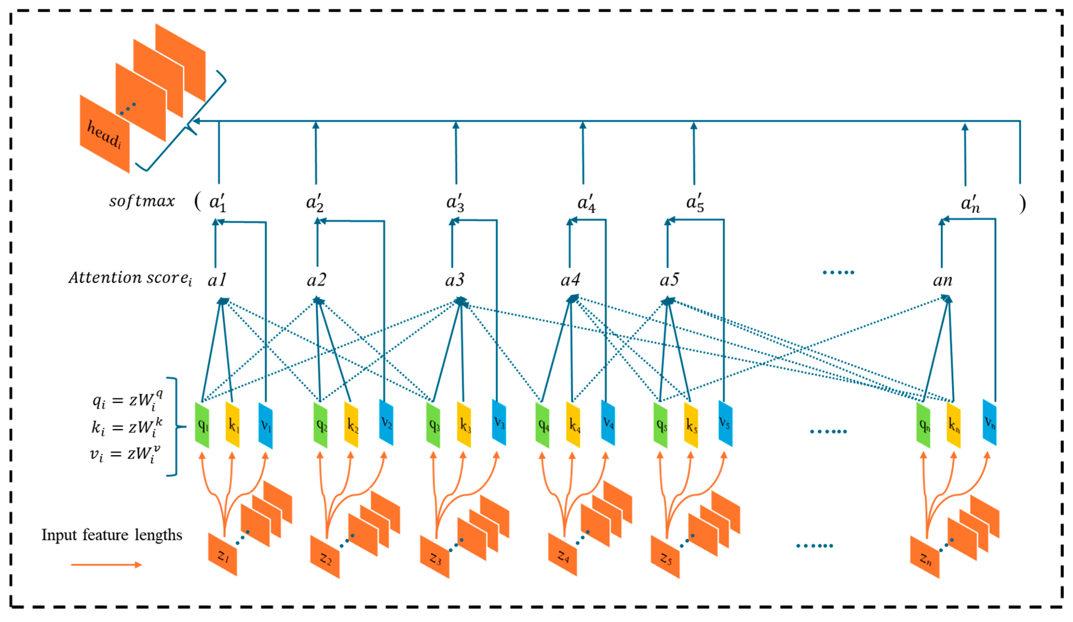
3.3. Multi-Head Attention in Model Architecture

In recent years, attention mechanisms have been widely applied across various domains, such as natural language processing, image recognition, and sequence data analysis, demonstrating their unique value in deep learning [46]. This involves three key components: Query (Q), representing the current focus; Key (K), a set of vectors for matching with the Query; and Value (V), a set of vectors containing information related to the Keys. Multi-head attention is an extension of the attention mechanism that splits the input into multiple ‘heads’, each performing an independent attention operation, then merging the outputs of all heads. According to Section 3.1, the features are reduced in dimensionality after the convolutional layer initially extracts them from the raw data. The processed data retains 60 impedance features for each cycle sample, denoted as $Z=\left(\mathrm{0,1},2,\dots ,59\right)$, and serves as the input of the multi-head attention mechanism. After the impedance feature is input, multiple attention heads will independently calculate and focus on different feature subsets, tracking the features while enhancing the model’s ability to learn different patterns. In addition, during the calculation process, different attention heads focus on different frequency ranges of the impedance data, and then adaptively assign weights to the features to reveal which features are more critical for SOH estimation, thereby improving prediction accuracy and enhancing the interpretability of the model. The computation process is as follows:

(1)

Linear Mapping: the input feature $Z$ is mapped through $Q_i$, $K_i$, and $V_i$ values, as shown in the following Equation (7),

$$Q_i=Z{W}_i^Q,K_i=Z{W}_i^K,V_i=Z{W}_i^V$$

(7)

where $i$ represents the $i$th head, and the $K_i$ vector is used to match the query vector $Q_i$. The final output is obtained by computing a weighted sum of the value vectors $V_i$, where the weights are determined by the matching scores. $W_i^Q$, $W_i^K$, and $W_i^V$ are learnable weight matrices, respectively.

(2)

Calculating Similarity Scores: for each head, the similarity score between the query and all keys is calculated as shown in Equation (8):

$$Attention scor{e}_i={\displaystyle \frac{Q_i{K}_i^T}{\sqrt{d_k}}}$$

(8)

The similarity score is represented by computing the dot product between $Q_i$ and $K_i^T$. $\sqrt{d_k}$ is used as a scaling factor to adjust the magnitude of the dot product scores. The final result is represented as a matrix of similarities between each query and all keys.

(3)

Normalizing Weights: to transform the scores into a probability distribution, the $softmax$ function is applied to the scores of each query, ensuring that all weights sum to 1, as shown in Equation (9):

$$Attention weight{s}_i=softmax\left(Attention scor{e}_i\right)$$

(9)

where $attention weight{s}_i$ represents the weights obtained for the $i$th head, achieved by applying the $softmax$ function to normalize the similarity scores $scor{e}_i$. Ultimately, which features have a greater impact on the model’s predictions depends on their weight distribution in each attention head.

(4)

Weighted Sum: the normalized weights are applied to the values to obtain the weighted output for each head, as shown in Equation (10),

$$hea{d}_i=Attention weight{s}_i{V}_i$$

(10)

where $hea{d}_i$ represents the weighted output for the $i$th head, calculated by applying the normalized weights $attention weight{s}_i$ to the corresponding values $V_i$.

(5)

Output Combination: the outputs from each head are combined and processed through a linear layer to generate the final result as follows:

$$MultiHead\left(Q,K,V\right)=Concat\left(hea{d}_1,\dots ,hea{d}_i\right)W^O$$

(11)

$MultiHead\left(Q,K,V\right)$ is the final output result, obtained by concatenating all heads ($hea{d}_1,\dots ,hea{d}_i$) and then applying a linear transformation. $W^O$ is a linear transformation matrix that maps the concatenated output to the target dimension.

3.4. Model Framework

This study proposes a model based on the Convolutional Gated architecture and multi-head attention mechanism. Compared to traditional single models, the integrated model combines the robustness of CNNs in handling noisy data and the strength of GRUs in capturing long-term dependencies in time series data, thereby enhancing overall comprehension and predictive ability. Three convolutional layers are used to extract features, and then the time information of the impedance features is input into the double-layer GRU network to identify the time information, and the multi-head attention mechanism is used to strengthen the extraction of impedance features. The estimation result is output through the fully connected layer. The detailed parameters of the network structure are shown in

Table 2. The summary of model parameters.

Layer	Other Parameters
Conv1d—1 (1, 32) BatchNorm1d (32) LeakyReLU ()	Kernel—1 (5)	Loss function (Huber)
Conv1d—2 (32, 64) BatchNorm1d (64) LeakyReLU ()	Kernel—2 (5)	Optimize (SGD)
Conv1d—3 (64, 128) BatchNorm1d (128) LeakyReLU () Maxpool (2)	Kernel—3 (5)
GRU—1 (128, 256) Dropout (0.3)
GRU—2 (256, 128) Dropout (0.1)
Multihead-attention (128) Dropout (0.1)	Num heads (4)
Linear (128, 64) Linear (64, 1)

.

4. Results and Discussion

4.1. Dataset Division

For training and testing the SOH estimation model, a six-fold cross-validation strategy is adopted to test the adaptability and robustness of the model on different cell data. Specifically, data from ten cells are used for training, and data from two other cells are used for testing. Among them, the training sets of folds one to four include cell capacity degradation data from the 25 °C, 35 °C, and 45 °C temperature environments. In the last two cross-validations, training samples from only two temperature environments are used to estimate the SOH prediction performance of batteries at 35 °C and 45 °C. This aims to validate the flexibility of the proposed algorithm framework in estimating battery SOH within the dataset. The specific division of each fold is shown in

Table 3. The data division of each fold.

Cross Validation	Fold1	Fold2	Fold3	Fold4	Fold5	Fold6
Cell ID	25C01	25C01	25C05	25C05	35C01	45C01
	35C01	35C02	45C01	45C02	35C02	45C02

.

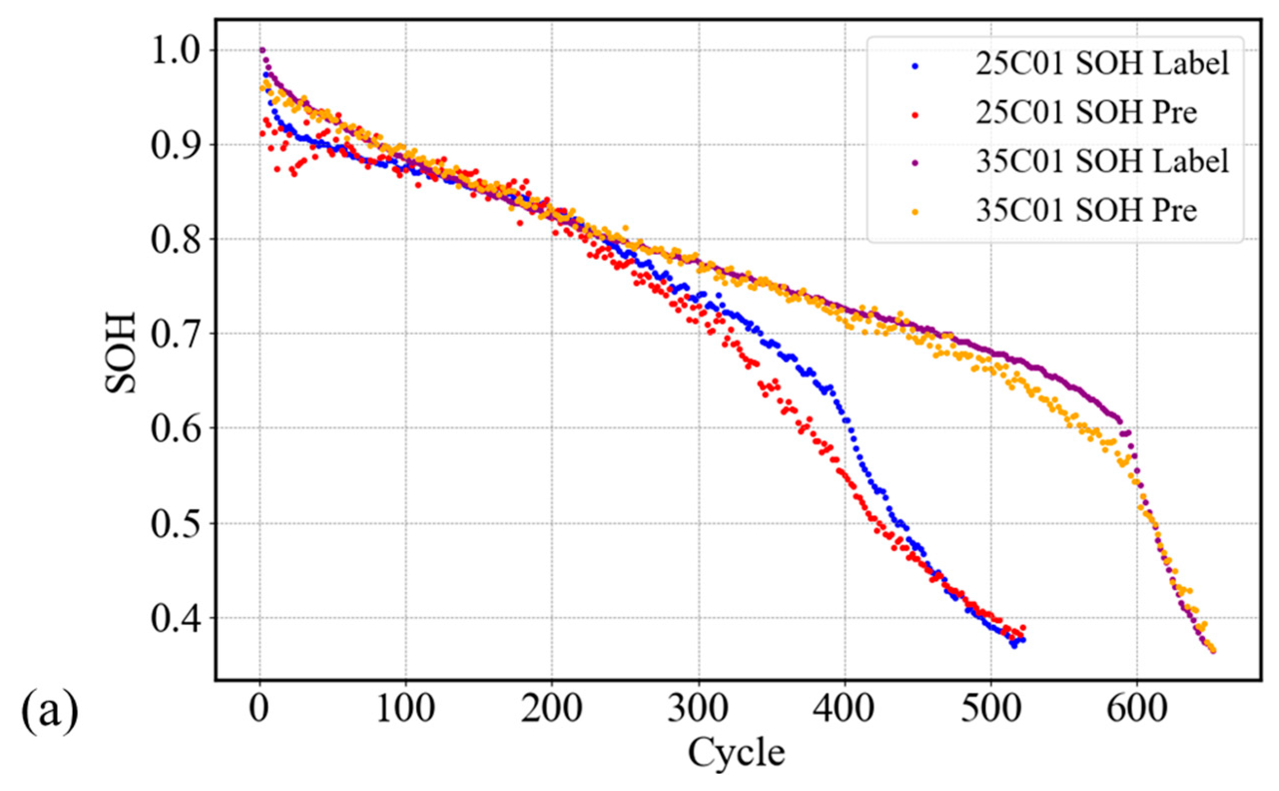
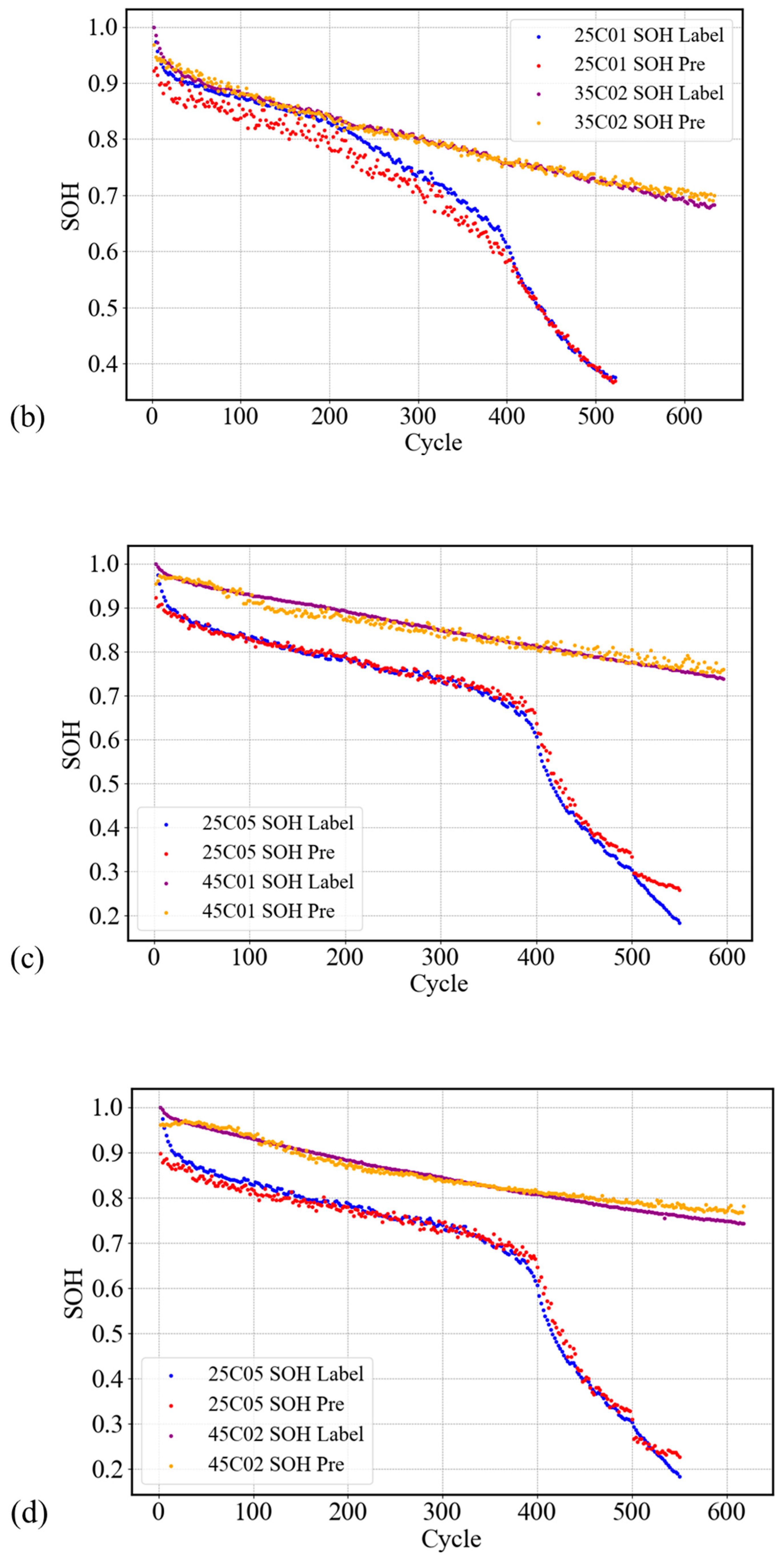
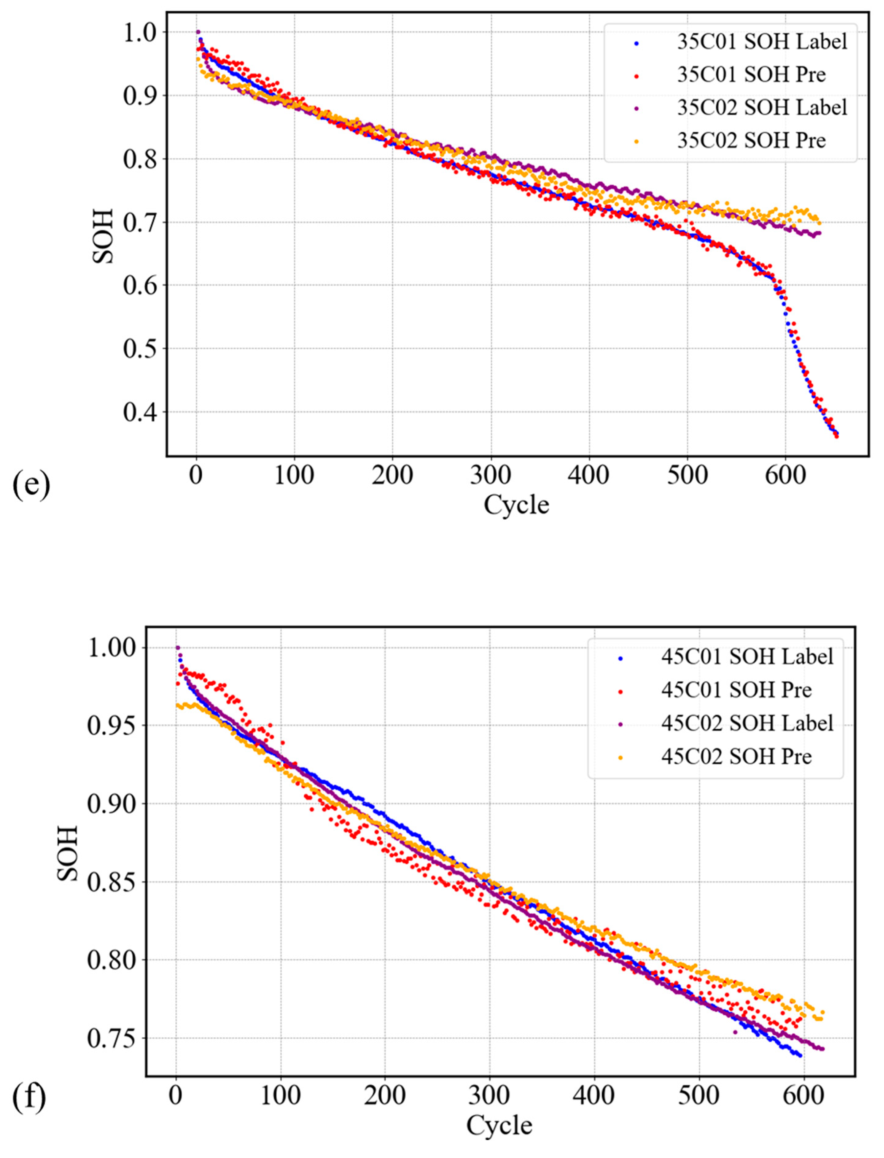
4.2. Analysis of Cross-Validation Results

In this study, the Huber function is used as the loss function to balance penalties for small and large prediction errors, enhancing the model’s robustness to outliers. Additionally, learning curves are plotted during the process to monitor changes in loss on the training and test sets, thereby evaluating the learning efficiency and potential overfitting of the model. The stochastic gradient descent (SGD) optimizer is used to adapt to dynamic changes during training. Figure 3 shows the overall process of SOH estimation.

Throughout the testing process of the model, RMSE, MAE, and the MAPE are used as evaluation indicators to comprehensively assess the prediction performance and accuracy. The loss function and evaluation metrics are as follows:

$$\mathrm{Huber} \mathrm{Loss}\left(y_i,{\widehat{y}}_i\right)=\left\{\begin{array}{l}{\displaystyle \frac{1}{2}}(y_i-{\widehat{y}}_i{)}^2 if|y_i-{\widehat{y}}_i|\le \delta \\ \delta \cdot (|y_i-{\widehat{y}}_i|-{\displaystyle \frac{1}{2}}\delta ) otherwise\end{array}\right.$$

(12)

$$RMSE=\sqrt{{\displaystyle \frac{1}{N}}\sum _{i=1}^N(y_i-{\widehat{y}}_i{)}^2}$$

(13)

$$MAE={\displaystyle \frac{1}{N}}\sum _{i=1}^N\left|y_i-{\widehat{y}}_i\right|$$

(14)

$$MAPE={\displaystyle \frac{1}{N}}\sum _{i=1}^N\left|{\displaystyle \frac{y_i-{\widehat{y}}_i}{y_i}}\right|\times 100\%$$

(15)

where $N$ represents the number of samples, $\delta$ is the threshold, $y_i$ denotes the actual battery SOH value, ${\widehat{y}}_i$ stands for the predicted battery SOH value, and $\overline{y}$ is the average of all actual values.

Figure 4 shows the comparison results between the predicted SOH and the actual SOH curves of different cells over their life cycle. In the first to fourth folds of cross-validation, the cells with more gentle capacity decay have an overall higher prediction accuracy. The prediction errors of the model vary among different batteries at different cycling stages (25C01, 25C05, 35C01, 35C02, 45C01, 45C02). It can be seen from Figure 4a–d that the prediction performance of the model is relatively accurate; especially when the SOH value is high (>0.7), the model can track the downward trend of the actual values well. The maximum average error occurs in the first fold of validation. This is due to significant capacity degradation in two cells during the first fold (with SOH dropping to around 0.4), as shown in Figure 4a; there are noticeable inflection points for the 25C01 battery around 350 cycles and for the 35C01 battery around 500 cycles. The prediction errors mainly occur in the later stages of battery aging, which indicates that the model has certain limitations when handling data from the rapid aging phase. However, the overall prediction accuracy remains high, and the maximum average MAPE value is maintained within 3%. To validate the model’s predictive capability for battery SOH across temperatures, the last two folds of cross-validation test data that did not appear in the training set (at 35 °C and 45 °C) are used. As analyzed in Section 2, the impedance curves of the batteries shift to the left in the early cycle stage at 45 °C, which is different from the other batteries in the dataset, resulting in large fluctuations in the model’s prediction errors for early SOH as shown in Figure 4f. However, the capacity degradation of the two batteries at 45 °C is basically consistent and relatively gentle, with the SOH dropping to 0.7 at about 600 cycles. The overall prediction accuracy is high, with an average RMSE of 0.5516 mAh, MAE of 0.4692 mAh, and MAPE of 1.35%. In the fifth fold of cross-validation, even when the capacity of the battery 35C02 decreases at the inflection point, it still maintains a high accuracy. As shown in Figure 2, among all battery samples, 25C01, 25C05, 25C07, and 35C02 have similar characteristics; all of them show obvious abrupt decreases in capacity in the later stages of the battery cycle. In addition, there are sufficient training samples of the same type in the validation of the fifth fold, where the cells at 25 °C are all used for training. The model is still able to effectively track the downward trend of the actual SOH values when predicting the batteries at 35 °C. The specific error data of each fold are shown in

Table 4. Different cross-validation results.

Model	Cross Validation	Cell ID	RMSE (mAh)	MAE (mAh)	MAPE (%)
CGMA-Net	Fold 1	25C01 35C01 Average	1.0217 0.5634 0.7926	0.7574 0.4013 0.5794	2.99 1.49 2.24
	Fold 2	25C01 35C02 Average	1.0919 0.3266 0.7093	0.9378 0.2412 0.5895	3.27 0.77 2.02
	Fold 3	25C05 45C01 Average	0.8258 0.5876 0.7067	0.5663 0.4747 0.5205	2.81 1.33 2.07
	Fold 4	25C05 45C02 Average	0.8073 0.5341 0.6707	0.5985 0.4373 0.5179	2.99 1.30 2.15
	Fold 5	35C01 35C02 Average	0.3345 0.4869 0.4107	0.2525 0.3778 0.3156	2.41 1.31 1.86
	Fold 6	45C01 45C02 Average	0.5727 0.5308 0.5516	0.4895 0.4488 0.4692	1.36 1.34 1.35

.

4.3. Ablation Experiments

In this section, ablation experiments are conducted to evaluate the model comprehensively, which is divided into six groups. The model structure obtained by ablation is used to predict the battery’s SOH. Among them, CNN and CNN-LSTM are model architectures that have been widely used in the same field [28,47]. Additionally, to further enhance the comparability and comprehensiveness of the experiments, the mainstream Transformer model is introduced as an additional baseline model. The six groups of models in the ablation experiment maintain the same hyperparameters as the proposed model to ensure fair comparison. Finally, the error analysis is performed by calculating the mean values of MAE, RMSE, and MAPE in each fold and comparing them with those of CGMA-Net. The specific error data are shown in

Table 5. The average RMSE (mAh), MAE (mAh), and MAPE (%) of ablation experiments models.

Cross Validation		Metrics	CGMA-Net	CNN	GRU	CNN-GRU	CNN-Attention	GRU-Attention	CNN-LSTM	Transformer
Fold1	25C01	MAE	0.7574	1.1032	1.0536	1.7649	1.3162	2.1073	1.5336	1.5671
		RMSE	1.0217	1.3960	1.1505	1.9633	1.6336	2.1438	1.6997	1.8548
		MAPE	2.99	4.89	4.18	6.66	4.93	8.45	5.95	6.42
	35C01	MAE	0.4013	0.9270	1.8104	1.2442	1.1186	1.4328	1.6023	1.1790
		RMSE	0.5634	1.3403	2.1833	1.6641	1.2435	1.7668	1.8142	1.5145
		MAPE	1.49	3.47	6.92	4.80	3.98	5.70	5.93	4.05
	Average	MAE RMSE MAPE	0.5794 0.7926 2.24	1.0151 1.3682 4.18	1.4320 1.6667 5.55	1.4956 1.8137 5.73	1.2174 1.4386 4.45	1.7700 1.9553 7.07	1.5679 1.7569 5.94	1.3730 1.6846 5.23
Fold2	25C01	MAE	0.9378	2.2811	3.3675	1.5786	1.8490	3.0064	0.8402	1.1989
		RMSE	1.0919	2.4838	3.7431	1.6951	2.0318	3.3559	0.9333	1.6072
		MAPE	3.27	8.48	11.97	5.79	6.85	10.79	3.16	4.83
	35C02	MAE	0.2412	0.6823	0.9022	0.6299	0.8565	0.9598	0.8748	1.1673
		RMSE	0.3266	0.7519	0.9332	0.7001	1.0192	0.9882	1.0256	1.3964
		MAPE	0.77	2.15	2.89	2.04	2.65	3.07	2.68	3.73
	Average	MAE RMSE MAPE	0.5895 0.7093 2.02	1.4817 1.6179 5.32	2.1349 2.3382 7.43	1.1043 1.1976 3.91	1.3527 1.5255 4.75	1.9831 2.1721 6.93	0.8575 0.9795 2.92	1.1831 1.5018 4.28
Fold3	25C05	MAE	0.5663	1.0634	0.8404	1.1455	1.4675	0.5944	1.2033	2.1234
		RMSE	0.8258	1.2323	1.1818	1.5297	1.6850	1.0950	1.4363	2.7911
		MAPE	2.81	5.62	5.87	7.65	7.13	4.90	7.36	10.76
	45C01	MAE	0.4747	1.8426	2.1769	0.4246	1.5927	1.5634	0.5540	1.0446
		RMSE	0.5876	2.2685	2.3353	0.5156	1.8769	1.7664	0.6632	1.2845
		MAPE	1.33	5.07	6.13	1.15	4.47	4.39	1.51	2.81
	Average	MAE RMSE MAPE	0.5205 0.7067 2.07	1.4530 1.7504 5.34	1.5087 1.7586 6.00	0.7850 1.0226 4.40	1.5301 1.7809 5.80	1.0789 1.4037 4.65	0.8786 1.0497 4.43	1.5840 2.0378 6.79
Fold4	25C05	MAE	0.5985	1.9677	1.6948	0.9784	1.3104	1.2250	1.0235	2.4121
		RMSE	0.8073	2.1827	2.0172	1.2712	1.6652	1.6711	1.5149	3.0633
		MAPE	2.99	8.93	9.17	6.23	8.45	8.49	7.35	14.01
	45C02	MAE	0.4373	0.9533	0.8212	0.5405	0.6954	0.9552	0.4983	1.3870
		RMSE	0.5341	1.1153	0.9036	0.6570	1.1120	1.0754	0.6657	1.6495
		MAPE	1.30	2.87	2.43	1.59	2.14	2.81	1.50	4.13
	Average	MAE RMSE MAPE	0.5179 0.6707 2.15	1.4605 1.6490 5.90	1.2580 1.4604 5.80	0.7594 0.9641 3.91	1.0029 1.3886 5.30	1.0901 1.3732 5.65	0.7609 1.0903 4.42	1.8995 2.3564 9.07
Fold5	35C01	MAE	0.2525	1.1867	1.7578	1.2736	0.8134	1.8474	0.9964	1.2641
		RMSE	0.3345	1.3648	1.8663	1.4067	0.9909	2.0332	1.0752	1.7900
		MAPE	2.41	4.52	6.56	4.29	2.90	6.99	3.65	4.77
	35C02	MAE	0.3778	0.8006	0.4282	0.7344	1.2130	0.5120	0.6451	1.3652
		RMSE	0.4869	0.8480	0.5038	0.9388	1.4198	0.5663	0.7299	1.6493
		MAPE	1.31	2.59	1.31	2.42	4.05	1.58	2.02	4.41
	Average	MAE RMSE MAPE	0.3156 0.4107 1.86	0.9936 1.1064 3.55	1.0930 1.1851 3.93	1.0040 1.1727 3.36	1.0132 1.2053 3.47	1.1797 1.2998 4.29	0.8207 0.9026 2.83	1.3146 1.7196 4.59
Fold6	45C01	MAE	0.4895	1.0895	1.6596	0.8339	1.6693	2.4081	0.3537	2.0117
		RMSE	0.5727	1.2415	1.7658	1.1916	2.4035	2.8839	0.5288	2.3453
		MAPE	1.36	3.02	4.60	2.22	4.64	6.55	0.98	5.64
	45C02	MAE	0.4488	0.8207	0.6787	0.6926	1.0958	0.7546	0.6475	0.8200
		RMSE	0.5308	0.9770	0.8094	0.7389	1.2233	0.9133	0.7467	1.0717
		MAPE	1.34	2.50	1.87	2.02	3.22	2.07	1.92	2.29
	Average	MAE RMSE MAPE	0.4692 0.5516 1.35	1.3151 1.1092 2.76	1.1692 1.2876 3.24	0.7633 0.9633 2.12	1.3825 1.1834 3.93	1.5814 1.8986 4.31	0.5006 0.6377 1.45	1.4158 1.7085 3.96

. Among the various models obtained from the ablation experiments, the GRU and the GRU model integrated with a multi-head attention mechanism show relatively poor overall prediction performance. For example, the GRU-attention model has an average MAPE of 7.07% in the first fold of cross-validation, and the GRU model has an average MAPE of 7.43% in the second fold, both of which are higher than those of the other models. Due to the lack of preliminary extraction of impedance information by the convolutional layer, the model has not effectively associated the impedance features with the battery capacity decay data. It may be due to the small sample size that the complex internal structure of the Transformer model overfits the limited sample data, resulting in overall mediocre performance. Its performance is particularly poor when predicting battery health at higher temperatures, especially at 35 °C, where the predictions exhibited large fluctuations, with an average MAPE of 4.59%, higher than those of other baseline models. The overall estimation performance of CNN-GRU and CNN-LSTM is relatively good, with the smallest difference from the proposed model, but they still exhibit relatively high errors in some folds (for example, the average MAPE of CNN-LSTM and CNN-GRU in fold one is 5.94% and 5.73%, respectively). When the test set does not include temperature data from the training set, CNN-GRU and CNN-LSTM still achieve high estimation accuracy. CNN-LSTM outperforms other baseline models in the fifth and sixth folds of cross-validation, with average MAPE values of 2.83% and 1.45%, respectively, and its performance is closest to the proposed framework. The specific average MAPE error visualization is shown in Figure 5.

We further discuss the computational costs required by different models, including the total number of parameters, model size, and the average training and testing times in the cross-validation for each model. Considering the resource-constrained and real-time data processing environment, attention should be paid to how these models can be deployed in practical applications. This section compares four commonly used baseline models with the proposed model. All experiments were conducted on a computer equipped with an NVIDIA GeForce RTX 4060 GPU and an AMD 7945HX CPU, with the detailed data presented in

Table 6. The parameters and computational costs of different SOH estimation models.

	Model Size	Total Parameters	Average Training Time	Average Testing Time
GRU	1751 kb	446,849	285.84 s	<0.1 s
CNN-GRU	1986 kb	505,025	1008.82 s	<0.2 s
CGMA-Net	2242 kb	571,073	1159.29 s	<0.2 s
CNN-LSTM	2560 kb	653,249	1239.52 s	<0.2 s
Transformer	3072 kb	783,953	1373.25 s	<0.2 s

.

The experimental results show that single-architecture models exhibit significantly higher computational efficiency. The GRU model, compared to the other four models, has the fewest parameters and the shortest average training time, with its training time being approximately one-quarter of the other integrated models. However, as mentioned in the ablation analysis in Section 4.3, the GRU model exhibits relatively high overall prediction errors. The limited number of parameters does not adequately capture the battery data across different temperatures in the dataset. The CNN-GRU and CNN-LSTM models in the ablation experiments showed relatively high overall prediction accuracy, with a small difference compared to CGMA-Net. This indicates that these two models perform well in balancing performance and computational efficiency. However, considering the real-time deployment of BMS and the limitations of computational resources, the GRU variant under the recurrent neural network framework is more suitable for deployment in resource-constrained environments. Although the Transformer architecture is widely used in many applications, due to its more complex network structure and the large number of weights and biased parameters during model training, the Transformer has not demonstrated good battery SOH prediction ability on this dataset with about 2000 samples. In addition, the average training time of different models is easily influenced by factors such as model complexity, training parameters, and dataset size. During the model testing process, since backpropagation and gradient updates are not required, the average testing time for battery SOH estimation across different models does not exceed 0.2 s, resulting in relatively low computational overhead.

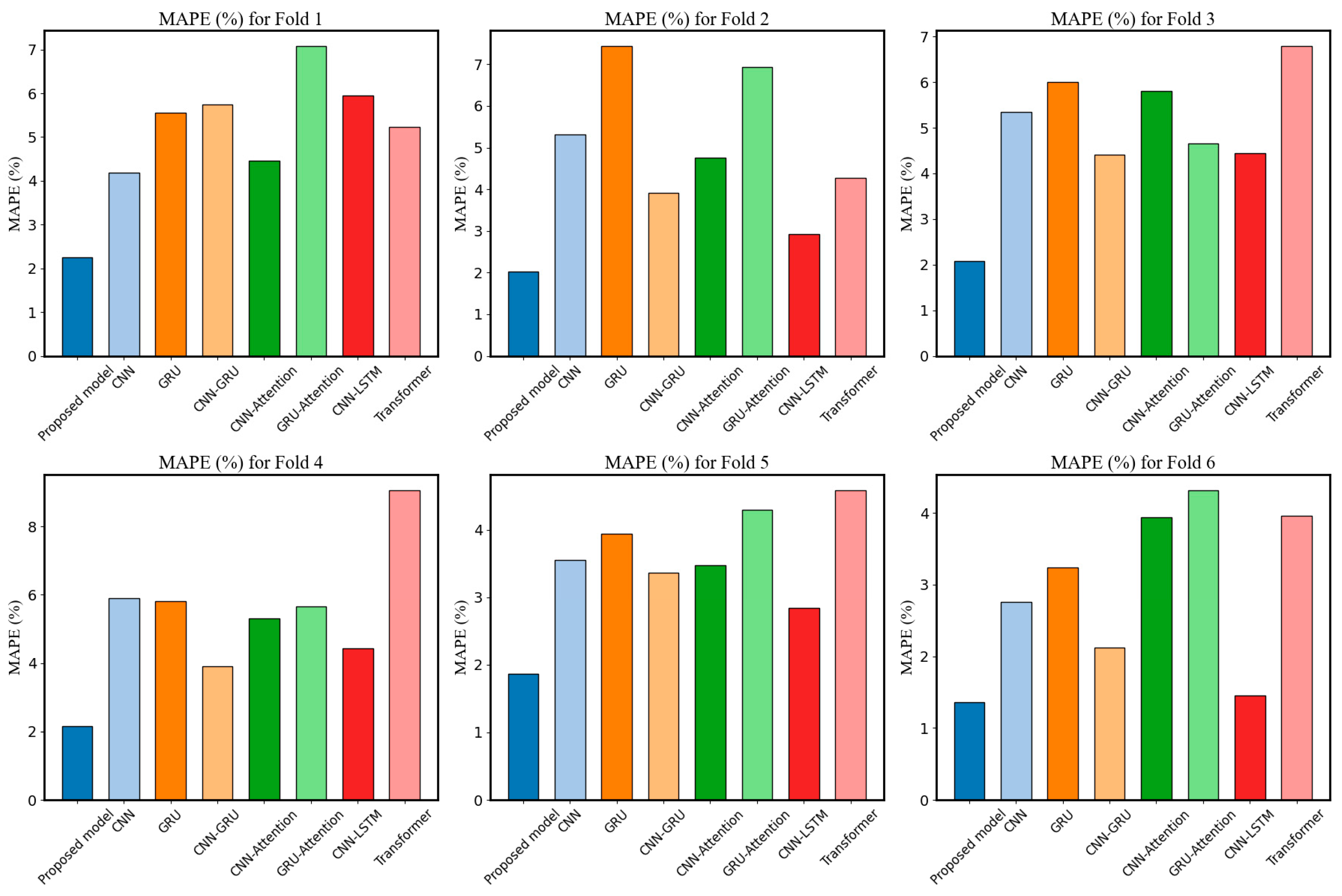
4.4. Comparison of the Advanced Models

In this section, a comparison with the baseline model is conducted using the model applied to the EIS data related to battery capacity degradation as a reference. Different studies have different experimental designs and methods; the temperature data contained in the references were selected and compared by calculating the mean error on the test set. RMSE and R² are used as the evaluation standards. In addition, considering the different units of error metrics used in various studies, the influence of dimensionality was removed to ensure a fair comparison. Ref. [27] proposed a novel ECM with an additional capacitor (ECMC). They first identified the parameters of the proposed ECMC based on EIS data, and then combined it with a data-driven approach to estimate the SOH. Li et al. [28] proposed a method that combines the ECM with electrochemical impedance spectroscopy data to estimate the SOH of lithium-ion batteries. The improved approach ensures the effectiveness of the ECM and enhances the accuracy of SOH estimation. Ref. [30] proposed an end-to-end deep learning architecture based on convolutional autoencoders (CAEs) and deep neural networks (DNNs) for feature extraction from electrochemical impedance spectroscopy (EIS) data. The impedance data are converted into 2D images for processing to estimate the SOH of lithium-ion batteries. Lin et al. [31] proposed an algorithm that combines a physical model with a deep learning framework (PIDL) for SOH prediction. This approach integrates EIS features and data fusion, while also exploring the model’s interpretability through domain knowledge and the predicted results. Wang et al. [32] proposed a framework called SSA-Net, which utilizes precise battery physical and chemical degradation information along with a bio-inspired spatiotemporal attention neural network. This framework simulates the transmission mechanism of brain neurons, achieving high gradient transmission efficiency while ensuring the accuracy of SOH estimation. Ref. [33] estimates SOH through the transformer architecture. Comparing the above method with the research in this paper, the specific error data are shown in

Table 7. Comparison of SOH estimation of baseline models.

Temperature	Model	RMSE	R2	References
25 °C	ECMC-GPR	0.0207	-	[27]
	ECM	0.0537	0.9374	[28]
	PIDL	0.0636	0.9500	[31]
	SSA-Net	0.0257	0.3828	[32]
	CGMA-Net	0.0275	0.9731	-
35 °C	ECMC-GPR	0.0131	-	[27]
	ECM	0.0691	0.9453	[28]
	CAE-DNN	0.0129	0.9657	[30]
	SSA-Net	0.0262	0.8711	[32]
	Transformer	0.6400	0.9400	[33]
	CGMA-Net	0.0105	0.9908	-

. Experimental results show that the proposed model performs well on the test set, especially in the processing results at 35 °C, where its SOH estimation error is lower than other baseline models. The ECMC-GPR model performs better than other models for the battery data at 25 °C. This may be due to the impact of the early use of ECM on the fitting accuracy of EIS data. However, compared with the error of CGMA-Net, it still has no obvious advantage, and its error value is below 0.01. The use of ECM to simulate large EIS data is not only computationally complex and time-consuming, but also heavily relies on prior knowledge and manual processing, which may limit its effectiveness in some cases.

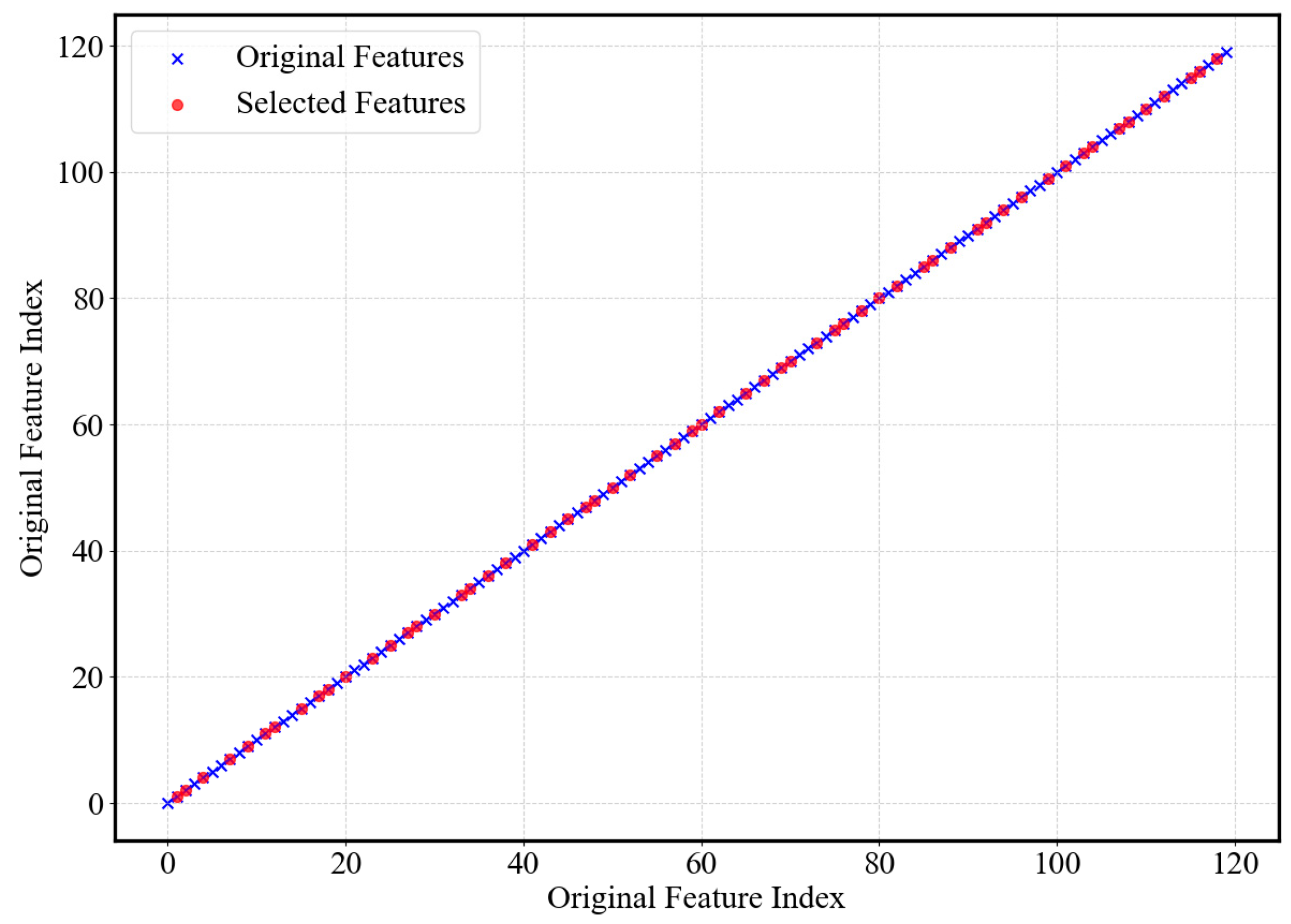
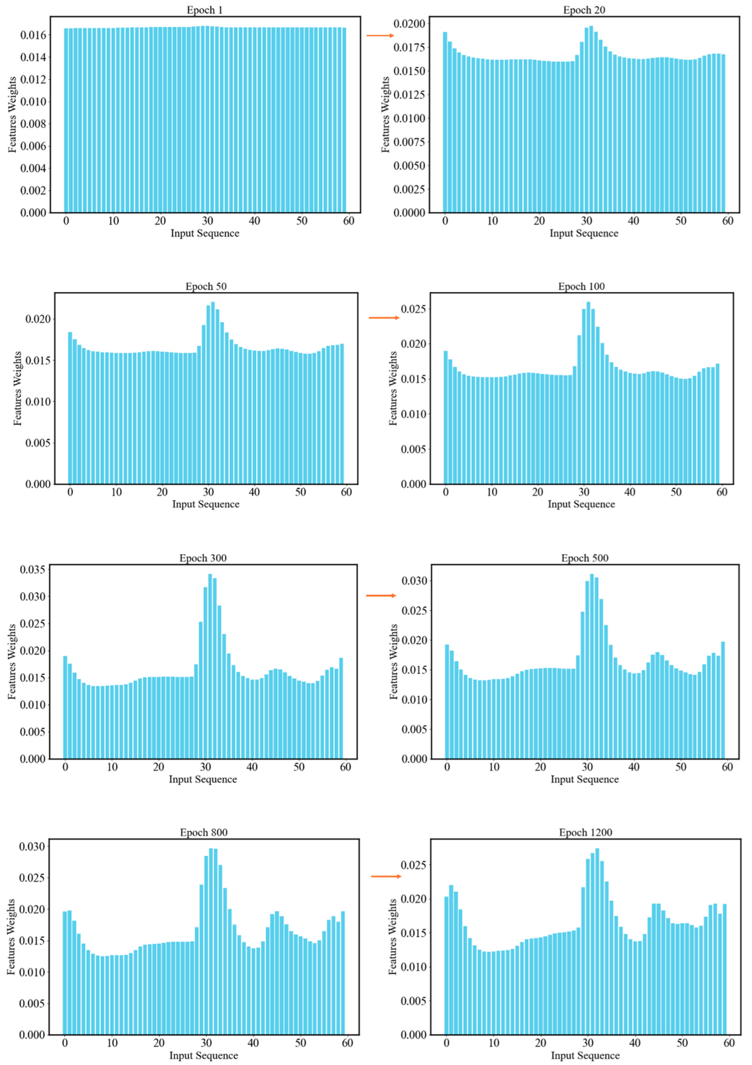
4.5. Interpretability Analysis Based on Attention Mechanism

This section will introduce the decision-making process of different impedance features based on the attention mechanism in detail to explore the interpretability of the model. In Section 3.1, the input features have been filtered, reducing the sequence length from 120 to 60. To determine the distribution of the selected 60 impedance features, the original impedance features are labeled, and the selected feature index is extracted through the convolutional framework, facilitating subsequent feature tracking. Additionally, considering that the experimental batteries in this dataset were tested across a frequency range of [0.02 Hz–20,000 Hz], the selected features remain evenly distributed from low to high frequencies to avoid deliberately emphasizing the contribution of data in a specific frequency range to the final prediction. In each cycle, 31 real impedance data points and 29 imaginary data points are ultimately extracted, which is close to a one-to-one ratio, to ensure fair competition between the real and imaginary parts. Subsequently, the contribution of EIS data at different frequencies is automatically determined through the attention framework. The selected EIS feature sequence and the original sequence are shown in Figure 6.

The labeled feature vector $Z$ is fed into the multi-head attention framework, where the model automatically initializes the weight matrices $W_i^Q$, $W_i^K$, and $W_i^V$. These matrices are matched with the input sequence to generate three vectors: query, key, and value. $q_i$ and $k_i$ are extracted, and the dot product of the two vectors is calculated to obtain the attention mechanism score. The same operation is applied to each feature, ultimately forming a score matrix. Subsequently, the attention score is input into the $softmax$ layer, which converts the data into a probability distribution to obtain the weight distribution of each feature. The attention weights are used to compute a weighted sum with the value vector, and the results of all head calculations are concatenated to form the final feature representation. The feature selection process of the attention mechanism framework is visualized in Figure 7. In this section, we extract the weight outputs from the $\odot$ layer and calculate the average attention weights across multiple attention heads to quantify the importance of each feature. By analyzing results from multiple epochs during model training, the average attention weights are visualized to observe the dynamic changes in the contribution of different features to SOH estimation. In addition, when the number of training epochs reaches around 1200, the SOH prediction accuracy on the test set has stabilized, with a correlation coefficient of (R²) approximately 0.98. Therefore, the parameter updates were stopped at 1200 epochs, as the training had converged. Figure 8 visualizes the dynamic change trend of EIS feature contribution.

From Figure 8, it can be seen that during the early stages of training (as shown in Epoch 1), the model assigned almost the same weight coefficients to the 60 input features, with the weight values for all features concentrated around 0.016. As training progresses, during the early stages (the first 50 epochs), there is a shift in the weight distribution across features from different frequency ranges. The features in the middle of the index gradually have a greater impact on the model’s decision, but the overall change in values is still not obvious, fluctuating within the range of 0.015 to 0.020. By the mid-training stage, there is a noticeable change in the distribution of features. The data located in the middle of the input sequence, the feature with indexes in the range of approximately [29,38], contribute the most and greatly influence the decision-making process of the model compared to the other features. These feature indices correspond to the data collected in the frequency range of 8.82 Hz to 28.41 Hz in the original EIS data. In the Nyquist diagram, the impedance data measured in the range of 10~100 Hz usually indicate changes in the mid-frequency region 48, which is reflected as a semicircle. As shown in the Nyquist plot in Section 2, as the number of cycles increases, the semicircle in the mid-frequency region gradually enlarges and shifts to the right, which is highly correlated with the battery capacity degradation pattern. The electrochemical characteristics in the mid-frequency region mainly represent the charge transfer process, which is significantly influenced by the electron exchange rate between the electrode surface and the solution, as well as the charge transfer impedance. This indicates that the dynamic changes in the charge transfer reaction and interfacial processes dominate the model’s inference process. As the number of training epochs increases, the contribution of features with earlier sequence indices gradually strengthens, as shown by the weight changes in epochs 800~1200 in the figure. The frequency range of index is from 9909 Hz to 20,004 Hz, corresponding to the high-frequency region. Its electrochemical characteristics are related to the capacitive response of the electrode surface and the conductivity of the electrolyte. In the Nyquist plot, it typically appears as a semicircle close to the x-axis, with the intersection point on the x-axis representing ohmic impedance. During the battery aging process, this semicircle shifts to the right, indicating a gradual increase in ohmic impedance. This is typically associated with the degradation of electrolyte impedance and the electrode interface. Although the contribution of high-frequency region features gradually increases in the later stages of training, the weight distribution values remain lower than the EIS data in the mid-frequency region, indicating that these features have a relatively limited role in the overall SOH prediction.

In this section, through the analysis of impedance spectra across different frequency ranges, the focus is on the variations in impedance responses across each frequency interval. It identifies which frequency ranges’ electrochemical characteristics dominate in battery SOH prediction, providing more accurate SOH monitoring indicators for the algorithm.

4.6. Future Research Directions and Prospects

This study uses the CGMA network architecture to achieve flexible estimation of battery SOH at 25 °C, 35 °C, and 45 °C in the dataset. Due to the relatively small sample size in the dataset, the temperature range of the battery test was conducted at three temperatures, which may be different from the complex and changeable conditions in the real world. Considering that environmental temperature is a key factor affecting battery aging, it can even lead to safety issues under certain extreme conditions. Future research should take into account the more variable environmental conditions during the use of electric vehicles, explore a wider range of battery types, and collect data from different battery samples to better adapt to a wider range of battery types and more complex operating conditions. In addition, the interpretability of deep learning models remains a challenge, especially when dealing with complex nonlinear relationships. The ways to enhance the model’s interpretability could be further explored in future research, enabling a better understanding of key factors that contribute to changes in battery SOH degradation.

5. Conclusions

In this study, a comprehensive deep learning framework of the CGMA network is proposed and applied to the SOH estimation of LIBs over their entire life cycle. EIS data contain rich electrochemical information about the internal state of the battery and can reflect its degradation characteristics. This framework can process EIS data automatically, achieving in-depth mining of the potential relationship between impedance features and battery degradation patterns, as well as the joint extraction of spatiotemporal features, without the need for complex manual feature engineering. The proposed framework was used to automatically track feature data. The interpretability of the model was explored by combining the electrochemical information represented by the internal battery with different weights assigned to EIS data by the model. In addition, the robustness and generalization ability of the model were verified by designing multiple cross-validation and ablation experiments, achieving flexible estimation of battery SOH in the dataset, and the SOH estimation errors of multiple models were calculated in detail. The experimental results show that the average RMSE and MAE values of the battery SOH prediction results were within 1 mAh, and the average MAPE was below 2.5%.

Future research should consider the actual usage scenarios of batteries and need to be validated in more battery types and under different operating temperatures. At the same time, we can delve deeper into the extraction techniques of electrochemical impedance spectroscopy features and consider integrating other algorithms to optimize the health state prediction of LIBs to ensure safety during battery usage.

References

1. Rajaeifar, M.A.; Ghadimi, P.; Raugei, M.; Wu, Y.; Heidrich, O. Challenges and recent developments in supply and value chains of electric vehicle batteries: A sustainability perspective. Resour. Conserv. Recycl. 2022, 180, 106144. [Google Scholar] [CrossRef]
2. Grey, C.P.; Hall, D.S. Prospects for lithium-ion batteries and beyond—A 2030 vision. Nat. Commun. 2020, 11, 6279. [Google Scholar] [CrossRef] [PubMed]
3. Habib, A.A.; Hasan, M.K.; Issa, G.F.; Singh, D.; Islam, S.; Ghazal, T.M. Lithium-ion battery management system for electric vehicles: Constraints, challenges, and recommendations. Batteries 2023, 9, 152. [Google Scholar] [CrossRef]
4. Zhou, L.; Lai, X.; Li, B.; Yao, Y.; Yuan, M.; Weng, J.; Zheng, Y. State estimation models of lithium-ion batteries for battery management system: Status, challenges, and future trends. Batteries 2023, 9, 131. [Google Scholar] [CrossRef]
5. Nuroldayeva, G.; Serik, Y.; Adair, D.; Uzakbaiuly, B.; Bakenov, Z. State of health estimation methods for Lithium-ion batteries. Int. J. Energy Res. 2023, 2023, 4297545. [Google Scholar] [CrossRef]
6. You, H.; Wang, X.; Zhu, J.; Jiang, B.; Han, G.; Wei, X.; Dai, H. Investigation of lithium-ion battery nonlinear degradation by experiments and model-based simulation. Energy Storage Mater. 2024, 65, 103083. [Google Scholar] [CrossRef]
7. Arora, P.; White, R.E.; Doyle, M. Capacity fade mechanisms and side reactions in lithium-ion batteries. J. Electrochem. Soc. 1998, 145, 3647. [Google Scholar] [CrossRef]
8. Ramadass, P.; Haran, B.; White, R.; Popov, B.N. Capacity fade of Sony 18650 cells cycled at elevated temperatures: Part I. Cycling performance. J. Power Sources 2002, 112, 606–613. [Google Scholar] [CrossRef]
9. Xia, L.; Najafi, E.; Bergveld, H.J.; Donkers, M.C.F. A computationally efficient implementation of an electrochemistry-based model for Lithium-ion batteries. IFAC PapersOnLine 2017, 50, 2169–2174. [Google Scholar] [CrossRef]
10. Li, J.; Lotfi, N.; Landers, R.G.; Park, J. A single particle model for lithium-ion batteries with electrolyte and stress-enhanced diffusion physics. J. Electrochem. Soc. 2017, 164, A874. [Google Scholar] [CrossRef]
11. He, H.; Xiong, R.; Fan, J. Evaluation of lithium-ion battery equivalent circuit models for state of charge estimation by an experimental approach. Energies 2011, 4, 582–598. [Google Scholar] [CrossRef]
12. Ding, X.; Zhang, D.; Cheng, J.; Wang, B.; Luk, P.C.K. An improved Thevenin model of lithium-ion battery with high accuracy for electric vehicles. Appl. Energy 2019, 254, 113615. [Google Scholar] [CrossRef]
13. Liu, X.; Li, W.; Zhou, A. PNGV equivalent circuit model and SOC estimation algorithm for lithium battery pack adopted in AGV vehicle. IEEE Access 2018, 6, 23639–23647. [Google Scholar] [CrossRef]
14. Luo, W.; Syed, A.U.; Nicholls, J.R.; Gray, S. An SVM-based health classifier for offline Li-ion batteries by using EIS technology. J. Electrochem. Soc. 2023, 170, 030532. [Google Scholar] [CrossRef]
15. Li, Y.; Zou, C.; Berecibar, M.; Nanini-Maury, E.; Chan, J.C.W.; Van den Bossche, P.; Van Mierlo, J.; Omar, N. Random forest regression for online capacity estimation of lithium-ion batteries. Appl. Energy 2018, 232, 197–210. [Google Scholar] [CrossRef]
16. Olabi, A.G.; Abdelghafar, A.A.; Soudan, B.; Alami, A.H.; Semeraro, C.; Al Radi, M.; Al-Murisi, M.; Abdelkareem, M.A. Artificial neural network driven prognosis and estimation of Lithium-Ion battery states: Current insights and future perspectives. Ain Shams Eng. J. 2023, 15, 102429. [Google Scholar] [CrossRef]
17. Qu, J.; Liu, F.; Ma, Y.; Fan, J. A neural-network-based method for RUL prediction and SOH monitoring of lithium-ion battery. IEEE Access 2019, 7, 87178–87191. [Google Scholar] [CrossRef]
18. Yang, N.; Song, Z.; Hofmann, H.; Sun, J. Robust State of Health estimation of lithium-ion batteries using convolutional neural network and random forest. J. Energy Storage 2022, 48, 103857. [Google Scholar] [CrossRef]
19. Sun, H.; Sun, J.; Zhao, K.; Wang, L.; Wang, K. Data-driven ICA-Bi-LSTM-combined lithium battery SOH estimation. Math. Probl. Eng. 2022, 2022, 9645892. [Google Scholar] [CrossRef]
20. Li, P.; Zhang, Z.; Xiong, Q.; Ding, B.; Hou, J.; Luo, D.; Rong, Y.; Li, S. State-of-health estimation and remaining useful life prediction for the lithium-ion battery based on a variant long short term memory neural network. J. Power Sources 2020, 459, 228069. [Google Scholar] [CrossRef]
21. Chen, Z.; Zhao, H.; Zhang, Y.; Shen, S.; Shen, J.; Liu, Y. State of health estimation for lithium-ion batteries based on temperature prediction and gated recurrent unit neural network. J. Power Sources 2022, 521, 230892. [Google Scholar] [CrossRef]
22. Li, Y.; Tao, J. CNN and transfer learning based online SOH estimation for lithium-ion battery. In Proceedings of the 2020 Chinese Control And Decision Conference (CCDC), Hefei, China, 22–24 August 2020; pp. 5489–5494. [Google Scholar] [CrossRef]
23. Hu, C.; Jain, G.; Zhang, P.; Schmidt, C.; Gomadam, P.; Gorka, T. Data-driven method based on particle swarm optimization and k-nearest neighbor regression for estimating capacity of lithium-ion battery. Appl. Energy 2014, 129, 49–55. [Google Scholar] [CrossRef]
24. Shen, S.; Sadoughi, M.; Chen, X.; Hong, M.; Hu, C. A deep learning method for online capacity estimation of lithium-ion batteries. J. Energy Storage 2019, 25, 100817. [Google Scholar] [CrossRef]
25. Li, Y.; Li, K.; Liu, X.; Wang, Y.; Zhang, L. Lithium-ion battery capacity estimation—A pruned convolutional neural network approach assisted with transfer learning. Appl. Energy 2021, 285, 116410. [Google Scholar] [CrossRef]
26. Zhang, Y.; Wik, T.; Bergström, J.; Pecht, M.; Zou, C. A machine learning-based framework for online prediction of battery ageing trajectory and lifetime using histogram data. J. Power Sources 2022, 526, 231110. [Google Scholar] [CrossRef]
27. Li, C.; Yang, L.; Li, Q.; Zhang, Q.; Zhou, Z.; Meng, Y.; Zhao, X.; Wang, L.; Zhang, S.; Li, Y.; et al. SOH estimation method for lithium-ion batteries based on an improved equivalent circuit model via electrochemical impedance spectroscopy. J. Energy Storage 2024, 86, 111167. [Google Scholar] [CrossRef]
28. Li, D.; Yang, D.; Li, L.; Wang, L.; Wang, K. Electrochemical impedance spectroscopy based on the state of health estimation for lithium-ion batteries. Energies 2022, 15, 6665. [Google Scholar] [CrossRef]
29. Galeotti, M.; Cinà, L.; Giammanco, C.; Cordiner, S.; Di Carlo, A. Performance analysis and SOH (state of health) evaluation of lithium polymer batteries through electrochemical impedance spectroscopy. Energy 2015, 89, 678–686. [Google Scholar] [CrossRef]
30. Obregon, J.; Han, Y.R.; Ho, C.W.; Mouraliraman, D.; Lee, C.W.; Jung, J.Y. Convolutional autoencoder-based SOH estimation of lithium-ion batteries using electrochemical impedance spectroscopy. J. Energy Storage 2023, 60, 106680. [Google Scholar] [CrossRef]
31. Lin, Y.H.; Ruan, S.J.; Chen, Y.X.; Li, Y.F. Physics-informed deep learning for lithium-ion battery diagnostics using electrochemical impedance spectroscopy. Renew. Sustain. Energy Rev. 2023, 188, 113807. [Google Scholar] [CrossRef]
32. Wang, H.; Li, Y.F.; Zhang, Y. Bioinspired spiking spatiotemporal attention framework for lithium-ion batteries state-of-health estimation. Renew. Sustain. Energy Rev. 2023, 188, 113728. [Google Scholar] [CrossRef]
33. Luo, K.; Zheng, H.; Shi, Z. A simple feature extraction method for estimating the whole life cycle state of health of lithium-ion batteries using transformer-based neural network. J. Power Sources 2023, 576, 233139. [Google Scholar] [CrossRef]
34. Tang, X.; Wang, Y.; Zou, C.; Yao, K.; Xia, Y.; Gao, F. A novel framework for Lithium-ion battery modeling considering uncertainties of temperature and aging. Energy Convers. Manag. 2019, 180, 162–170. [Google Scholar] [CrossRef]
35. Leng, F.; Tan, C.M.; Pecht, M. Effect of temperature on the aging rate of Li ion battery operating above room temperature. Sci. Rep. 2015, 5, 12967. [Google Scholar] [CrossRef] [PubMed]
36. Zhang, Y.; Tang, Q.; Zhang, Y.; Wang, J.; Stimming, U.; Lee, A.A. Identifying degradation patterns of lithium-ion batteries from impedance spectroscopy using machine learning. Nat. Commun. 2020, 11, 1706. [Google Scholar] [CrossRef] [PubMed]
37. Lazanas, A.C.; Prodromidis, M.I. Electrochemical impedance spectroscopy—A tutorial. ACS Meas. Sci. Au 2023, 3, 162–193. [Google Scholar] [CrossRef]
38. Mc Carthy, K.; Gullapalli, H.; Ryan, K.M.; Kennedy, T. Use of impedance spectroscopy for the estimation of Li-ion battery state of charge, state of health and internal temperature. J. Electrochem. Soc. 2021, 168, 080517. [Google Scholar] [CrossRef]
39. Zhao, B.; Lu, H.; Chen, S.; Liu, J.; Wu, D. Convolutional neural networks for time series classification. J. Syst. Eng. Electron. 2017, 28, 162–169. [Google Scholar] [CrossRef]
40. Canizo, M.; Triguero, I.; Conde, A.; Onieva, E. Multi-head CNN–RNN for multi-time series anomaly detection: An industrial case study. Neurocomputing 2019, 363, 246–260. [Google Scholar] [CrossRef]
41. Liu, S.; Ji, H.; Wang, M.C. Nonpooling convolutional neural network forecasting for seasonal time series with trends. IEEE Trans. Neural Netw. Learn. Syst. 2019, 31, 2879–2888. [Google Scholar] [CrossRef]
42. Liu, C.L.; Hsaio, W.H.; Tu, Y.C. Time series classification with multivariate convolutional neural network. IEEE Trans. Ind. Electron. 2018, 66, 4788–4797. [Google Scholar] [CrossRef]
43. Hewamalage, H.; Bergmeir, C.; Bandara, K. Recurrent neural networks for time series forecasting: Current status and future directions. Int. J. Forecast. 2021, 37, 388–427. [Google Scholar] [CrossRef]
44. Liu, Y.; Gong, C.; Yang, L.; Chen, Y. DSTP-RNN: A dual-stage two-phase attention-based recurrent neural network for long-term and multivariate time series prediction. Expert Syst. Appl. 2020, 143, 113082. [Google Scholar] [CrossRef]
45. Guo, T.; Xu, Z.; Yao, X.; Chen, H.; Aberer, K.; Funaya, K. Robust online time series prediction with recurrent neural networks. In Proceedings of the 2016 IEEE International Conference on Data Science and Advanced Analytics (DSAA), Montreal, QC, Canada, 17–19 October 2016; pp. 816–825. [Google Scholar] [CrossRef]
46. Niu, Z.; Zhong, G.; Yu, H. A review on the attention mechanism of deep learning. Neurocomputing 2021, 452, 48–62. [Google Scholar] [CrossRef]
47. Pradyumna, T.K.; Cho, K.; Kim, M.; Choi, W. Capacity estimation of lithium-ion batteries using convolutional neural network and impedance spectra. J. Power Electron. 2022, 22, 850–858. [Google Scholar] [CrossRef]
Figure 1. Variation in the electrochemical impedance spectroscopy graph of cells across different cycles. (ac) The cells are 25C01, 35C02, and 45C02, respectively.
Energies 18 01385 g001
Figure 2. Capacity degradation curves of cells at different temperatures.
Energies 18 01385 g002
Figure 3. The overall process framework of the SOH estimation.
Energies 18 01385 g003
Figure 4. Predicted and actual values of the cells SOH. (af): Visualization of six-fold cross-validation.
Energies 18 01385 g004aEnergies 18 01385 g004bEnergies 18 01385 g004c
Figure 5. The cross-validation results of average MAPE for different models.
Energies 18 01385 g005
Figure 6. The distribution of original feature and selected feature sequences.
Energies 18 01385 g006
Figure 7. The decision-making process of the attention mechanism for different EIS data.
Energies 18 01385 g007
Figure 8. Dynamic changes in attention scores of different features.
Energies 18 01385 g008