Analysis of the Mechanical Stability of Power Transformer Windings Considering the Influence of Temperature Field

Abstract

The power transformer is a critical primary device in the power grid, and the verification of its winding mechanical stability is of paramount importance in ensuring the safe and stable operation of the power grid. In the conventional numerical calculation methods for verifying the mechanical stability of power transformer windings, the influence of temperature variations at the winding hot spots on winding mechanical stability has not been taken into account. In reality, factors such as the transformer’s operating load rate, ambient temperature, and the duration of short-circuit fault currents passing through will affect the mechanical stability margin of the transformer windings. Under conditions such as winding aging, deformation, or other reasons, the transformer windings may become unstable due to material parameter degradation, leading to insufficient mechanical stability margin. This paper analyzes the mechanical stability of power transformer windings considering the impact of the temperature field. Initially, a numerical model for calculating short-circuit currents in transformers was established to compute the short-circuit current under three-phase short-circuit-to-ground conditions as an excitation. Subsequently, a 3D electromagnetic force finite element calculation model was developed to determine the electromagnetic forces experienced under this condition. The results of the calculated electromagnetic forces were then used in a numerical calculation method to assess the mechanical stability of the windings. Furthermore, a 3D transformer electromagnetic–thermal flow finite element model was created to calculate the steady-state temperature rise under various operating conditions of the transformer. This model is validated through transformer temperature rise tests, and transient temperature rises under different operating conditions are calculated. The obtained data are fitted using the nonlinear least squares method to derive a fitting function for the winding hot spot temperature concerning load rate, ambient temperature, and short-circuit time. Taking into consideration the influence of temperature on the yield strength and modulus of elasticity of transformer winding materials, the variation in mechanical stability margin of transformer windings due to temperature effects is analyzed. Additionally, the operating domain for preventing the transformer from becoming unstable under three-phase short-circuit impacts is calculated for different degrees of material parameter degradation. This method provides an effective reference for transformer design and operation, demonstrating clear practical value.

1. Introduction

Power transformers are important primary equipment in modern power grids, responsible for voltage transformation and energy transmission. In the event of a transformer short-circuit fault, especially a three-phase short-circuit-to-ground fault, a very large short-circuit current flows through the transformer windings. Under the action of the short-circuit current, the transformer windings will experience significant electromagnetic forces. If the electromagnetic forces exceed a certain limit, the mechanical stability of the transformer windings can be compromised, leading to deformation, tilting, bending, and other instability issues [1]. Typically, during the design stage, transformer mechanical stability is verified and calculated to ensure the rationality of the design. However, conventional verification methods [2] do not consider the influence of temperature characteristics of transformer winding materials [3,4] on the mechanical stability. Therefore, these methods are often used for predelivery verification. Considering the temperature characteristics of winding materials, the mechanical stability margin may change compared to predelivery verification. When transformer materials degrade due to aging, deformation, or other reasons, the mechanical stability margin may become too small due to temperature variations, potentially leading to instability under short-circuit conditions. This study aims to consider the temperature field variations in transformer windings under different operating conditions and analyze the mechanical stability of power transformer windings by accounting for temperature-dependent yield strength and elastic modulus parameters.

Research on the mechanical stability of transformer windings has advanced significantly. Standards such as GB1094.5 and IEC60076-5 [5,6] specify stress value standards for verifying the mechanical stability of transformer windings, but these standards do not provide explicit stress value calculation expressions. Currently, for calculating the radial and axial stability of transformer windings, most researchers use relevant models and theories from material mechanics for analysis. Li Kaiqi [7] utilized a fixed-supported beam model to solve the superstatic problem and calculate the stress values in the axial and radial directions of transformer windings. Ou Qiang [8] and others considered manufacturing process deviations and material aging, proposing an equivalent support stiffness theory to calculate and analyze the radial buckling stability of transformer windings. Amit Bakshi [9] and others treated the winding portion between two supports as an arcuate arch hinged at both ends to determine the buckling critical stress of transformer windings supported by braces. These studies focus on solving the mechanical stability of windings using different material mechanics models. However, they often provide a fixed mechanical stability margin without considering the influence of temperature on material parameters. In reality, operating conditions and environments for transformers are variable, and with aging, deformation, or other reasons, material parameters inevitably degrade. Conventional numerical methods for verifying the mechanical stability of transformer windings do not consider the influence of temperature. Hence, this study aims to calculate and analyze the impact of temperature variations on the mechanical stability of transformer windings under multiple influencing factors.

To analyze the impact of temperature on the mechanical stability of transformer windings, it is crucial to first be able to calculate the temperature field of the windings accurately. Currently, the mainstream approach for calculating transformer temperature fields involves using computational fluid dynamics (CFD) [10,11,12,13,14,15]. This method integrates various numerical calculation methods such as the finite element method, finite volume method, least squares finite element method [16], inverse wind finite element method [17], inverse wind finite volume method [17], and others to achieve high-precision calculations of transformer temperature fields.

This study employs the finite element method to compute the temperature field of transformers. Due to the short duration of the short-circuit process, it is challenging to experimentally validate the transient process. Therefore, this research initially calculates the steady-state temperature rise in transformers under different conditions and validates the steady-state finite element temperature field model of transformers with transformer short-circuit temperature rise tests. Subsequently, using the steady-state temperature field output as the initial state, the transient temperature rise in transformers under short-circuit excitations is computed. The parameters affecting the temperature rise are then fitted with functions to obtain a fitting function for the hot spot temperature. Finally, this fitting function is utilized to analyze the influence of transformer winding material temperature characteristics on the mechanical stability margin of transformers. The study results reveal the extent and patterns of temperature influence on the mechanical stability of transformer windings, providing a method to analyze the mechanical stability margin of transformer windings considering the impact of temperature field, which is crucial for verifying the mechanical stability of operating transformers.

2. Theoretical Model of Transformer Windings

2.1. Theoretical Modeling of Transformer Electromagnetic Fields

In order to carry out a multiphysics field analysis of transformers, the electromagnetic field involved in transformers should be analyzed first.

In this paper, a three-dimensional solution algorithm based on the T-Ω bit group [18,19] is used to solve the low-frequency three-dimensional transient field problem. The electric vector T and the scalar potential Ω are defined as follows in Equation (1):

$$\begin{array}{c}\mathit{J}=\nabla \times \mathit{T}\\ \mathit{H}=\mathit{T}-\nabla \Omega \end{array}$$

(1)

where J is the current density and H is the magnetic field strength.

Disregarding the displacement current in the conductor, the control equation in the conducting part at this time is shown in Equation (2) below.

$$\nabla \times {\displaystyle \frac{1}{\sigma }}\nabla \times \mathit{T}+\mu {\displaystyle \frac{\partial \mathit{T}}{\partial t}}-\mu {\displaystyle \frac{\partial \nabla \Omega }{\partial t}}=0$$

(2)

The control equations in the region of non-conductive parts and multi-turn coils at this point are shown in Equation (3) below.

$$\nabla \cdot \left[\mu \left(-\nabla \Omega +\mathit{T}\right)\right]=0$$

(3)

Among them, σ is electrical conductivity, S/m; and μ is magnetic permeability, H/m.

During operation, the windings of a transformer are subjected to Lorentz forces, resulting from the combined excitation of winding currents and leakage magnetic fields. The formula for Lorentz force is given by Equation (4).

$$\mathit{F}=q\left(\mathit{E}+\mathit{V}\times \mathit{B}\right)$$

(4)

where F is the Lorentz force vector, N; q is the electric charge, C; E is the electric field strength vector, N/C; and B is the magnetic induction strength vector, T.

From the basic theory of power system analysis [20,21], it is known that when a short-circuit occurs in a power system, the short-circuit impulse current can be calculated by the following Equation (5):

$$i_{\mathrm{im}}=I\times k\times \sqrt{2}$$

(5)

where i_im is the short-circuit impulse current, A; I is the short-circuit periodic current RMS value, A; and k is the short-circuit impulse coefficient, the value of which is determined by the ratio of transformer and the system reactance value and resistance value.

For thermodynamic problems, when the power transformer operates, the heat source is mainly from copper losses of the transformer windings and core losses. It can be seen from classical circuit theory and the relevant theory of electrical engineering [22] that the copper loss of each phase can be calculated by following Equation (6).

$$P_{\mathrm{coil}}=I_{\mathrm{coil}}^2{R}_{\mathrm{cu}}$$

(6)

where P_coil is copper losses, kW; I_coil is the current flowing through the winding, A; and R_cu is the winding resistance, Ω.

Transformer no-load losses are generated mostly by the transformer core losses, which is calculated as follows in Equation (7):

$$P_{\mathrm{Fe}}=k_{\mathrm{h}}f{B}_{\mathrm{m}}^{\beta }+k_{\mathrm{c}}{f}^2{B}_{\mathrm{m}}^2+k_{\mathrm{e}}{f}^{1.5}{B}_{\mathrm{m}}^{1.5}$$

(7)

where P_Fe is the core loss, kW; and k_h, k_c, k_e, and β are the pending coefficients, determined by the magnetization curve of the ferromagnetic material. For a specific silicon steel sheet, the above pending coefficients are frequency-independent constants.

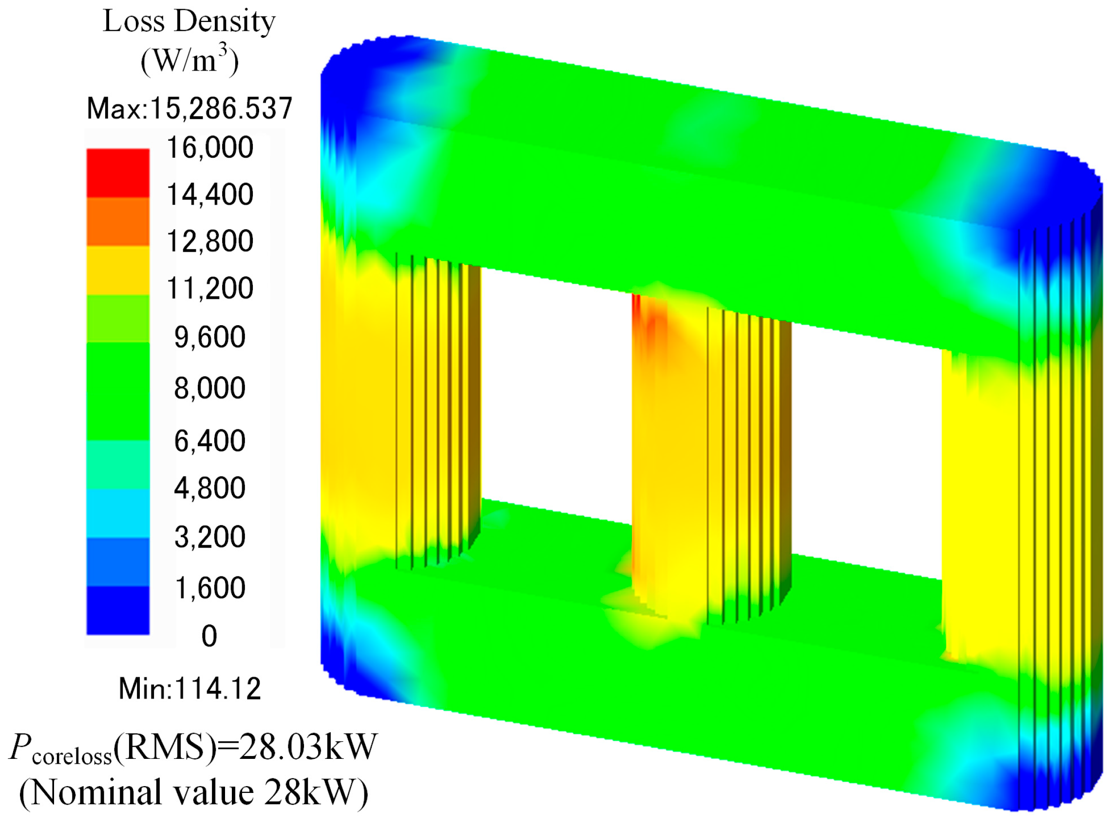
2.2. Theoretical Modeling of Transformer Heat-Flow Field

The following heat transfer equations were used for the solid domain [23,24]:

$$\nabla ·\left(\lambda \nabla T\right)+Q=\rho \mathrm{c}{\displaystyle \frac{\partial T}{\partial t}}$$

(8)

where T is the temperature, K; λ is the thermal conductivity, W/(m·K); Q is the internal heat generation rate, W/m³; ρ is the density of the material, kg/m³; c is the specific heat capacity, J/(kg·°C); and t is the time, s.

For the fluid domain, convective heat transfer plays a more dominant role compared to heat conduction. The transformer oil flow is approximated as an incompressible fluid, and its mass conservation equations, momentum conservation equations, and energy conservation equations are shown as follows in Equations (9)–(11):

$${\displaystyle \frac{\partial \rho }{\partial t}}+\nabla \cdot \left(\rho u\right)=0$$

(9)

$$\begin{array}{c}{\displaystyle \frac{\partial }{\partial \mathrm{t}}}\left(\rho \mathit{u}\right)+\nabla \cdot \left(\rho \mathit{u}\times \mathit{u}\right)=-\nabla p+u{\nabla }^2\mathit{u}\\ +g(\rho -pref)\end{array}$$

(10)

$${\displaystyle \frac{\partial }{\partial \mathrm{t}}}\left(\rho c_{\mathrm{p}}T\right)+\nabla \cdot \left(\rho c_{\mathrm{p}}\mathit{u}T\right)=\nabla \cdot k\nabla T$$

(11)

where ▽ refers to the Nabla operator, m⁻¹; u refers to fluid velocity vector, m/s; ρ refers to the fluid density, kg/m³; g refers to gravity acceleration constant, m/s²; c_p refers to specific heat capacity, J/(kg·K); T refers to temperature of transformer oil, K; k refers to thermal conductivity of the fluid, W/(m·K); and p refers to the fluid pressure, Pa.

The temperature distribution is affected by the heat conduction generated by the core, coil, and transformer oil convection, and the surface heat flux q_c is introduced to calculate the effect of convective heat transfer, which is calculated as shown in Equation (12) below.

$$q_{\mathrm{c}}=h\left(T-T_{\mathrm{ref}}\right)$$

(12)

where h is the heat transfer coefficient, W/m²·K; T is the solid surface temperature; and T_ref is the fluid temperature, K.

For a smooth wall surface, the convective relation is used to estimate convective coefficients, of which the empirical formulate is as follows:

$$h=N{u}_m{\displaystyle \frac{\lambda }{L}}$$

(13)

$$N{u}_m={\left[{\displaystyle \frac{6}{R_a^{\ast }}}+{\displaystyle \frac{1.88}{{\left(R_a^{\ast }\right)}^{0.4}}}\right]}^{-0.5}$$

(14)

$$R_{\mathrm{a}}^{\ast }={\displaystyle \frac{{\rho }^{2}g\beta c_p{b}^5{q}_w}{\mu L{\lambda }^2}}$$

(15)

where Nu_m is the Nusselt number; L is the characteristic length, m; $R_a^{*}$ is the Rayleigh number; β is the thermal expansion coefficient, m/k; b is the width of the vertical oil channel, m; q_w is heat flux per unit area; and μ refers to the dynamic viscosity of the fluid, Pa·s.

3. Transformer Mechanical Stability Analysis

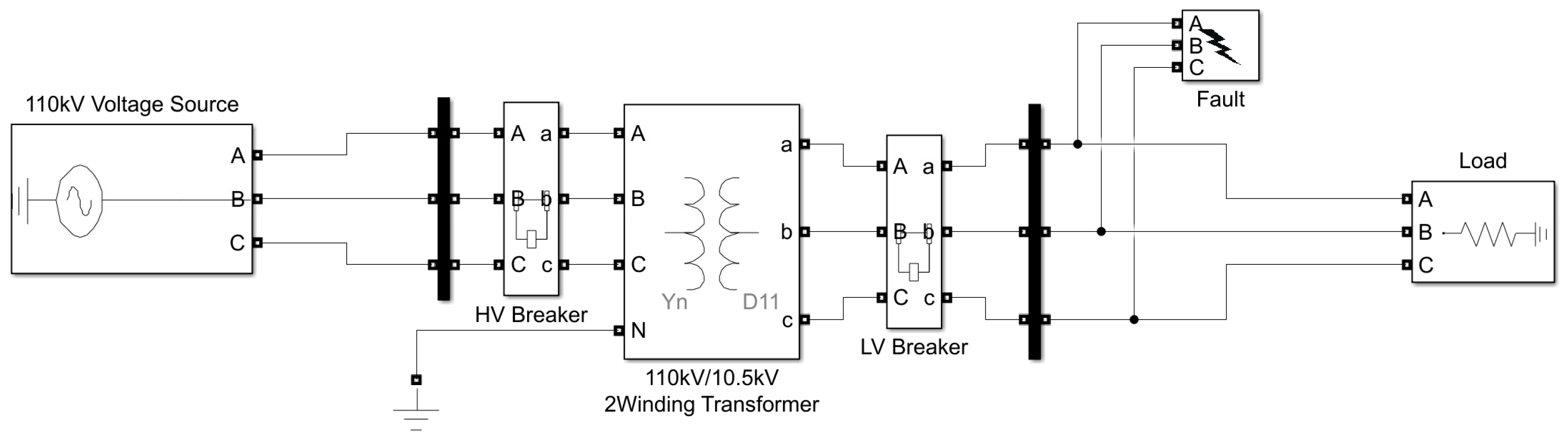
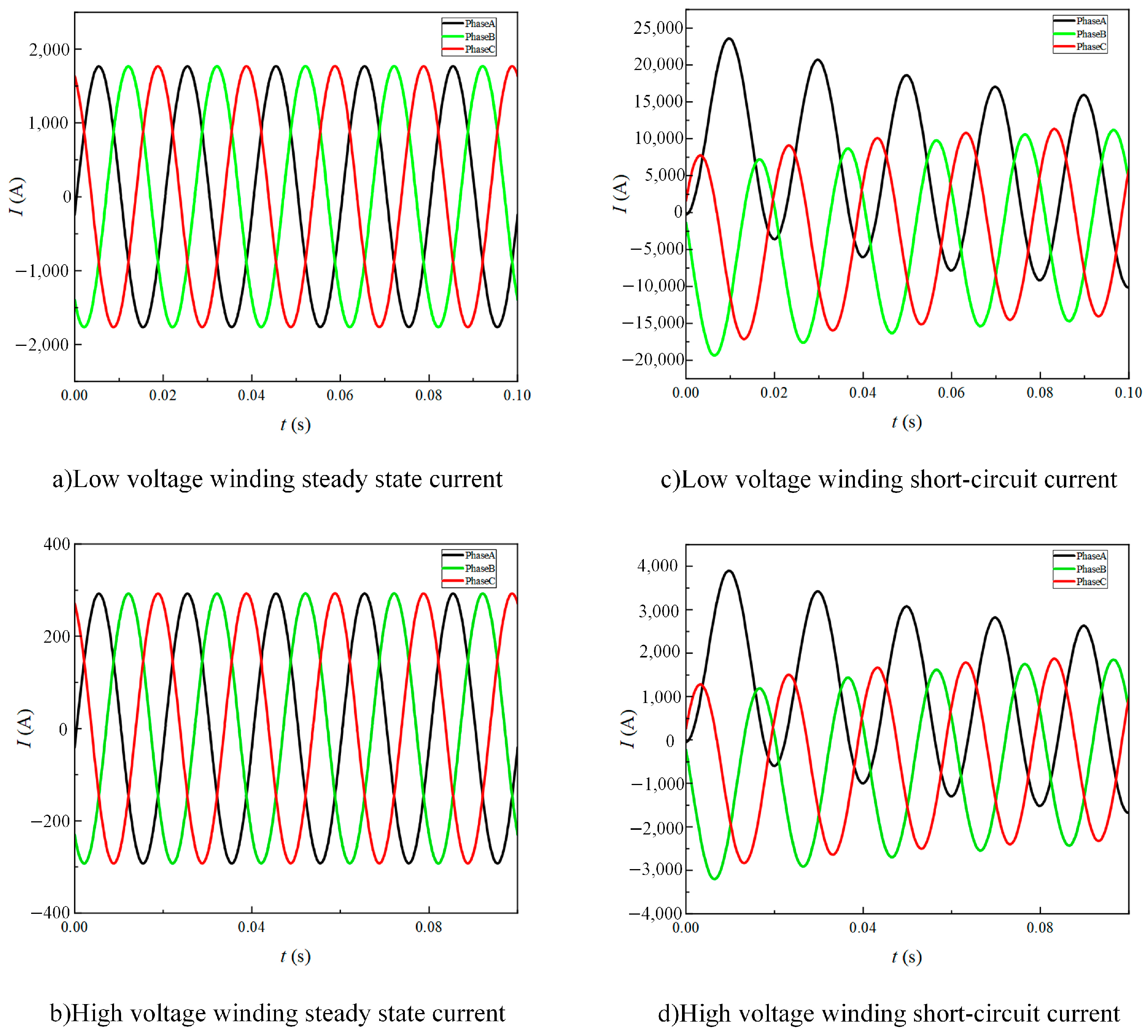
3.1. Transformer Winding Current Calculation Model

To facilitate the incorporation of the electromagnetic–temperature field coupling model’s excitations and to analyze steady-state and transient currents under different operating conditions, this study utilizes MATLAB/Simulink of R2020b version simulation software. Specifically, for the two-winding power transformer model SFZ-40000/110 manufactured by Shenyang Transformer Research Institute in Shenyang, China, a transformer winding current calculation model is established to compute steady-state currents during normal operation and transient currents during three-phase short-circuit conditions. The model is illustrated in Figure 1.

The detailed model settings are shown in

Table 1. SFZ-40000/110 transformer short-circuit current calculation model parameter settings.

Components	Parameters	Value
110 Kv Voltage Source	Nominal voltage	110 kV
	Nominal frequency	50 Hz
	Connection type	Yg
SFZ-40000/110 Transformer	Nominal voltage	110/10.5
	Nominal frequency	50 Hz
	Connection type	YNd11
	Nominal capacity	40 MVA
	LV winding R	0.010032 Ω
	LV winding L	9.212 × 10−4 H
	HV winding R	0.50364 Ω
	HV winding L	0.1011 H
	Excitation R	4,321,42.86 Ω
	Excitation L	481.44 H
Load	Nominal voltage	10.5 kV
	Nominal frequency	50 Hz
	Connection type	Yg
	Nominal active power	40 MVar
	Nominal reactive power	0
Circuit-Breaker	Breaker resistance	0 Ω
	Snubber resistance	1 × 106 Ω
Fault	Fault resistance	0.001Ω
	Snubber resistance	1 × 106 Ω

.

The transformer winding currents are calculated for five cycles (0.1 s) under rated operating conditions and three-phase short-circuit conditions. The steady-state currents of the transformer’s low and high voltage side windings are shown below, respectively, in Figure 2a and Figure 2b. And the short-circuit currents of the transformer’s low and high voltage side windings are shown, respectively, in Figure 2c and Figure 2d.

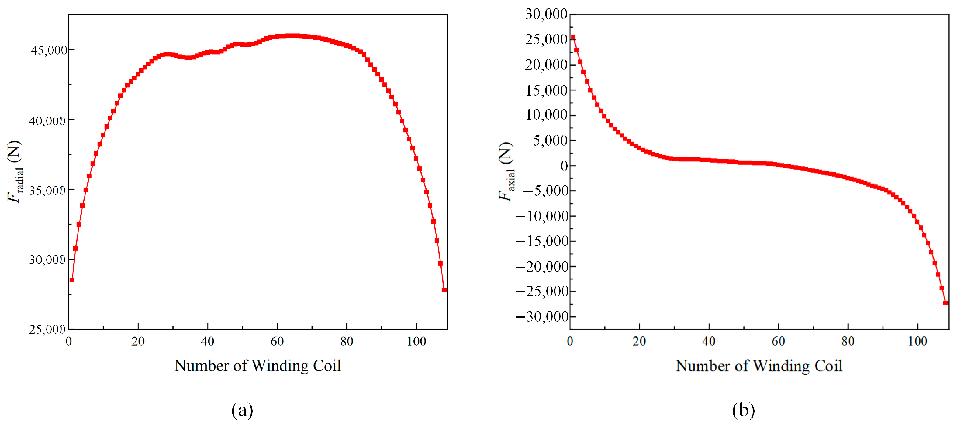
3.2. Finite Element Modeling and Analysis of Transformer Electromagnetic Force Fields

In this study, electromagnetic field finite element calculations are conducted using ANSYS/Maxwell. of 2024R1 version For the two-winding power transformer model SFZ-40000/110, the electrical parameters and dimensional parameters are presented in

Table 2. SFZ-40000/110 transformer electrical and dimensional parameters.

Num	Parameters	Configuration
1	Connection group	YNd11
2	Nominal voltage	110 kV/10.5 kV
3	Nominal frequency	50 Hz
4	Nominal capacity	40 MVA
5	No-load loss	28 kW
6	No-load current percentage	0.2
7	Wire diameter (HV/LV)	86.5 mm/90 mm
8	Winding height	1220 mm
9	Tank (length × width × height)	4750 mm × 1620 mm × 2730 mm

.

To simplify the computational analysis, the model is simplified as follows [14,25]:

(1)

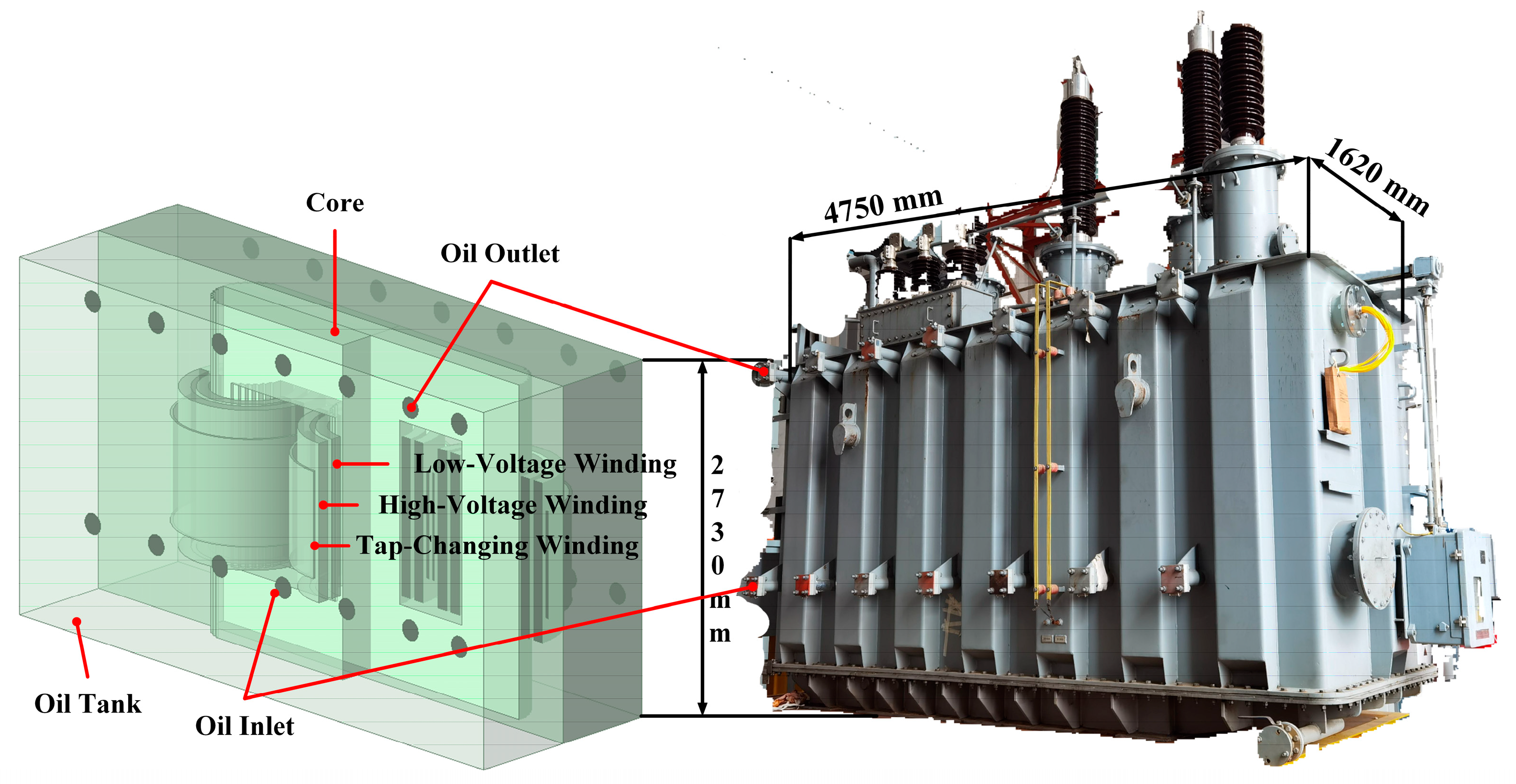
The model retains only the core, windings, and tank structure.

(2)

The oil ducts between the windings are neglected, and each phase winding is simplified to a hollow cylindrical structure.

(3)

The cooling fin structures are ignored, with only the oil inlet and outlet retained. Other components on the surface of the tank are neglected, as well as the thickness of the tank walls.

(4)

The core is treated as a whole, disregarding its laminated silicon steel structure.

The electromagnetic field finite element model of the transformer established in this study is illustrated in Figure 3.

To analyze the mechanical stability of transformer windings, it is necessary to first examine the short-circuit electromagnetic forces acting on them. Labeling the windings from the lower end of the low-voltage phase A winding to the upper end as numbers 1 to 109, the radial and axial forces at 0.01 s are depicted in the wire diagram below as Figure 4. Radial forces are considered positive in the direction toward the center, while axial forces are positive in the upward direction from the lower end.

From the above figure, it is evident that when the winding is subjected to short-circuit transient currents, the maximum value of the radial short-circuit force occurs in the middle of the winding, compressing toward the center. The maximum value of the axial force, on the other hand, is observed at both ends, compressing toward the middle.

3.3. Mechanical Stability of Transformers

For the mechanical stability of transformer windings, there are established standards such as IEC 60076-5 and GB 1094.5 that provide regulations on this matter. Regarding the low-voltage winding of the SFZ-40000/110 transformer under study in this paper, the corresponding stress and verification standards are presented in

Table 3. Transformer mechanical stability verification stresses and criteria.

Num	Stress	Criteria
1	mean hoop compressive stress	σt1 ≤ 0.35 Rp0.2
2	radial bending stress	σbr ≤ 0.7 Rp0.2
3	free buckling critical stress	σt1 ≤ σcr
4	compressive stress on radial spacers	σact ≤ 80 MPa
5	axial bending stress	σAL ≤ 0.9 Rp0.2

.

These stresses are currently difficult to measure directly through technical means. Generally, when the transformer is manufactured, the relevant formulas in the field of material mechanics are used for calculation. For each of the stresses involved in the above table, the equations are as follows [7]:

(1)

Mean hoop compressive stress

$${\sigma }_{\mathrm{t}1}={\displaystyle \frac{F_{\mathrm{r}}}{2\pi \cdot A_{\mathrm{cu}}}}$$

(16)

where σ_t1 is the average ring compression stress, MPa; F_r is the maximum radial force, N; and A_cu is the winding cross-sectional area, mm².

(2)

Radial bending stress

For a line cake between two pads, the radial bending stress is shown in the following equation:

$${\sigma }_{\mathrm{br}}={\displaystyle \frac{F_{\mathrm{r}}{l}^2}{2\pi D{t}_{\mathrm{v}}^2{w}_{\mathrm{v}}}}$$

(17)

where σ_br is the radial bending stress, MPa; l is the length of the winding between the two radial pads, mm; t_v is the radial width of the winding, mm; and w_v is the axial height of each wire pancake, mm.

(3)

Free buckling critical stress

$${\sigma }_{\mathrm{cr}}={\displaystyle \frac{E}{4}}\cdot {\left({\displaystyle \frac{t_{\mathrm{v}}}{R}}\right)}^2$$

(18)

where σ_cr is the free buckling limit stress, MPa; R is the average radius of the winding, mm; and E is the modulus of elasticity of the wire.

(4)

Compressive stress on radial spacers

$${\sigma }_{\mathrm{act}}={\displaystyle \frac{F_{\mathrm{a}}}{A_{\mathrm{z}}}}$$

(19)

where F_a is the axial force of the winding, N; A_z is the effective area of the pad, mm²; and σ_act is the axial compressive stress of the pad, N/mm².

(5)

Axial bending stress

$${\sigma }_{\mathrm{ba}}={\displaystyle \frac{F_{\mathrm{a}}{l}^2}{2\pi D{t}_{\mathrm{v}}{w}_{\mathrm{v}}^2}}$$

(20)

where σ_ba is the radial bending stress, MPa.

In the numerical computation of transformer mechanical stability verification, the values of winding yield strength and elastic modulus are typically set as fixed constants based on the transformer design temperature. For the SFZ-40000/110 transformer considered in this case, at its design temperature of 348.15 K, the yield strength (R_p0.2) is set at 160 MPa and the elastic modulus (E) is set at 125 GPa. Based on these values, the calculated stresses and their corresponding limits for the mechanical stability verification of the transformer windings are presented in

Table 4. Transformer mechanical stability verification stress calculations.

Num	Calculated Value (MPa)	Critical Value (MPa)
1	σt1 = 21.43	≤56
2	σbr = 2.24	≤112
3	σcr = 1800	≥21.43
4	σact = 3.39	≤80 MPa
5	σba = 15.22	≤144

.

4. Mechanical Stability Analysis of Power Transformer Windings by Counting and Temperature Field

This paper employs ANSYS/AEDT Icepak of 2024R1 version for thermal field finite element calculations. The model comprises steady-state and transient calculation components, where the results of the steady-state calculation serve as the initial condition for the transient calculation.

Considering operating conditions at a 100% load rate and winding resistance values based on a design temperature of 348.15 K, with steady-state current as the model excitation, the transformer winding copper losses and core losses are computed. Given the symmetry of the current values in the three phases, the analysis of copper losses is conducted for both low-voltage phase A and high voltage phase A, resulting in corresponding copper loss curves and a comparison with theoretical values shown in Figure 5.

It can be seen that the deviation of the copper loss calculated by this model from the theoretical value is very small, while the distribution of the core loss under this condition and its comparison with the rated value is shown in Figure 6.

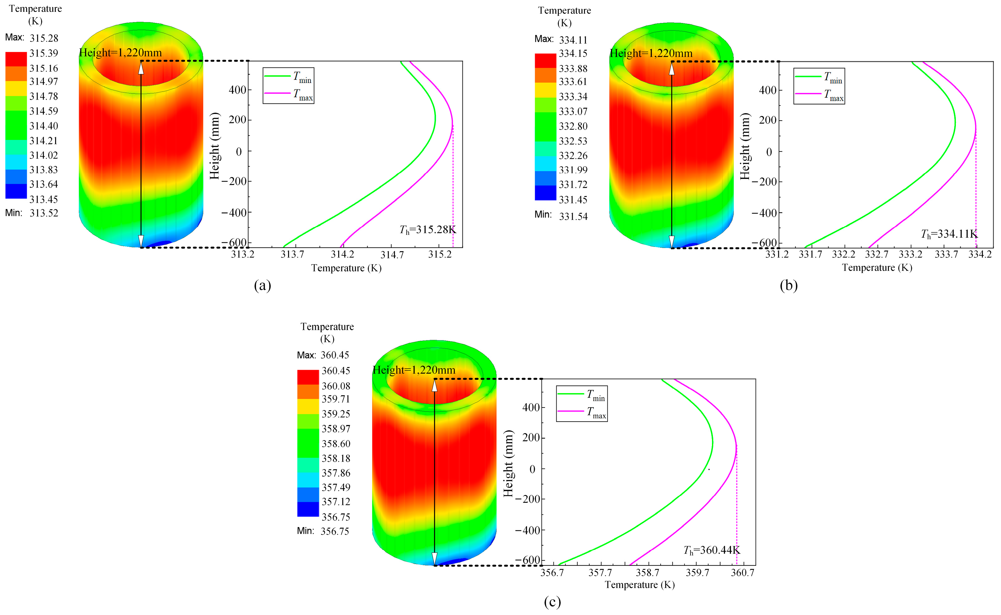
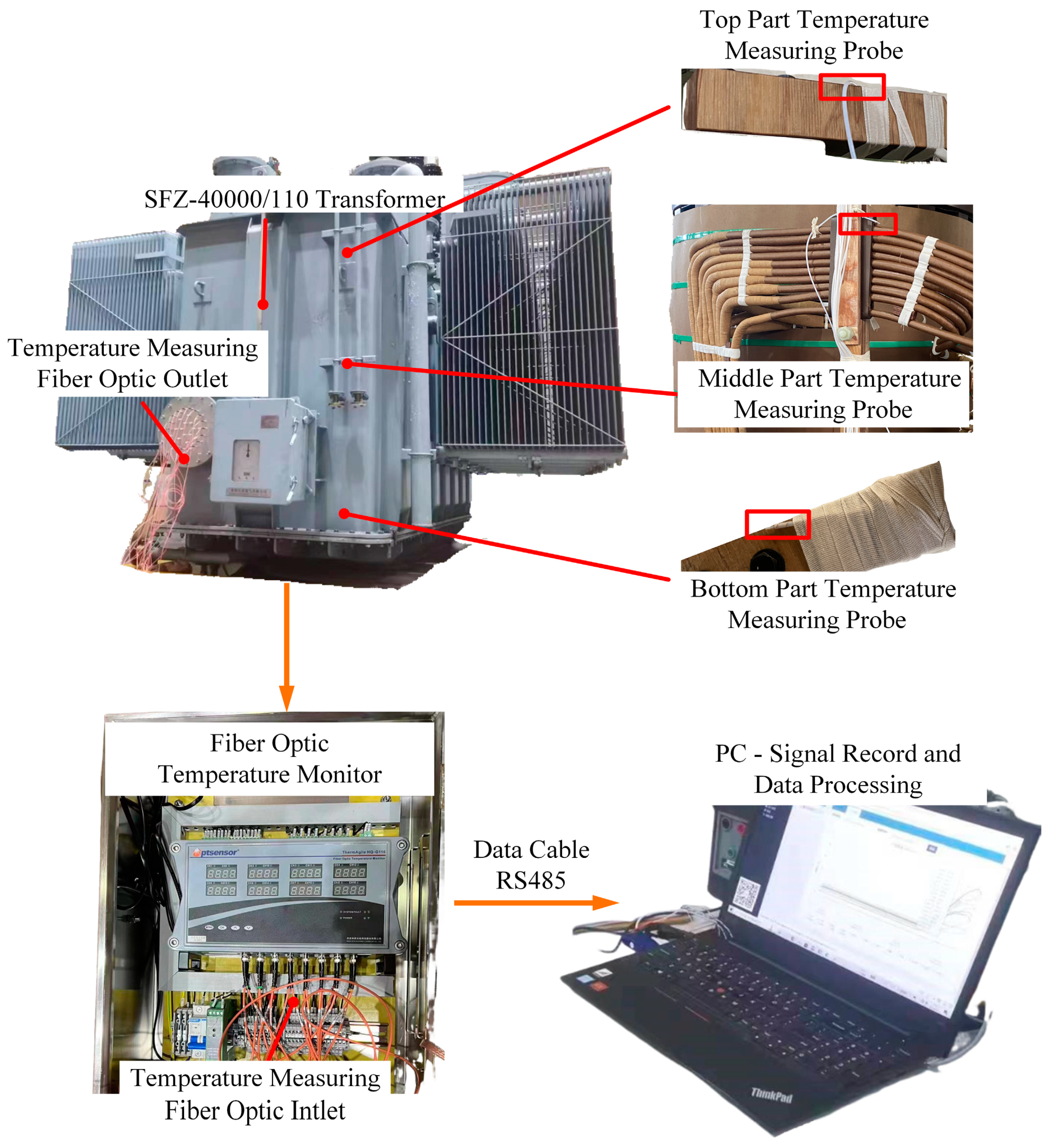
4.1. Transformer Heat-Flow Steady-State Field Calculations and Their Experimental Validation

For the steady-state calculation model, the excitation utilized consists of the copper losses in the windings and the core losses. The fluid domain is computed using a turbulent flow model, while the thermal radiation boundaries are modeled using the discrete ordinates radiation model. The oil inlet flow velocity is set at 0.8 m/s, and the oil outlet is defined as a pressure boundary.

In order to verify the validity of the method, the working conditions at which the model is calculated should be consistent with the subsequent experimental working conditions. As the transformer will then be experimented at 50%, 75%, 100% load rate and an ambient temperature of 293.15K, the winding copper losses and core losses are employed as excitation at load rates of 50%, 75%, and 100%, with an ambient temperature of 293.15K for steady-state temperature field calculations. And the subsequent experiments are The temperature distribution of the intermediate phase of the low-voltage winding under these three operating conditions is chosen for the analysis of hot spots in the transformer windings. The temperature distributions and the line chart showing the minimum and maximum temperatures at the same height section of the winding under 50%, 75%, and 100% load rates for the intermediate phase of the low-voltage winding are depicted in Figure 7. Here, T_min represents the minimum temperature at the same height section of the winding, T_max denotes the maximum temperature at the same height section of the winding, and T_h indicates the hot spot temperature of the winding:

As can be seen from the above figure, the simulated values of the winding hot spot temperature at 50%, 75%, and 100% load rates are 315.28 K, 334.11 K, and 360.44 K, respectively.

In order to verify the steady-state thermal field calculation model, a transformer winding temperature rise test was carried out with an SFZ-40000/110 oil-immersed transformer, and the test was carried out in the form of braced slotted embedded optical fiber, with the specific test apparatus and optical fiber measuring point detector layout as shown in Figure 8.

The experimental process is divided into two stages. The first stage is the preheating stage: to rapidly increase the transformer’s temperature, reduce the overall test duration, and conduct preheating before the formal experiment begins, heating the transformer temperature to a relatively high level. The second stage is the loading stage, where the transformer is subjected to 50%, 75%, and 100% load rates. The fiber optic temperature measurement point at 90% height of phase A winding is approximated as the hot spot temperature. The experiment continues for 1 h if the hourly temperature rise in all temperature measurement points and the top layer of oil are less than 1 K. During this hour, all temperature values at fiber optic points and the top layer oil temperature are recorded every 10 min. The steady-state value of the hot spot temperature within this final hour is considered as the experimental result.

The hot spot temperature curve was made according to the experimental data, as shown in Figure 9.

From the figure above, it is evident that the experimental values of the transformer winding hot spot temperatures at 50%, 75%, and 100% load rates are 318.75 K, 334.35 K, and 362.45 K, respectively.

The comparison of the experimental values of the transformer winding hot spot temperatures, which are 318.75 K, 334.35 K, and 362.45 K, with the simulated values of 315.28 K, 334.11 K, and 360.44 K, shows errors of 3.47 K, 0.24 K, and 2.01 K. Due to the simplification of the model, in order to improve the computational efficiency of the model, there is a certain deviation between the experimental data and the simulation data. At the same time, the use of optical fiber embedded in transformer windings for temperature measurement, due to the tightness of the optical fiber to the windings and the sensitivity difference in the optical fiber material to temperature, will also introduce a certain measurement error. However, the error between the experimental data and the simulation data above shows that the overall error is within 5 K, which is acceptable for engineering applications. Hence, the thermal field simulation model for this transformer is validated.

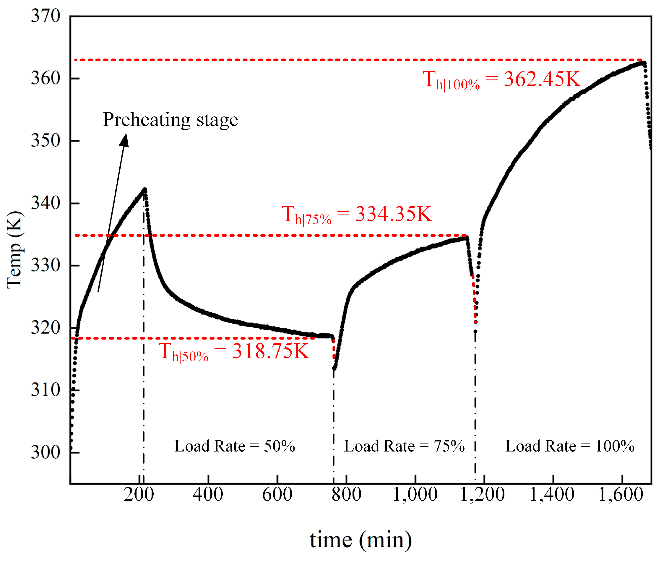
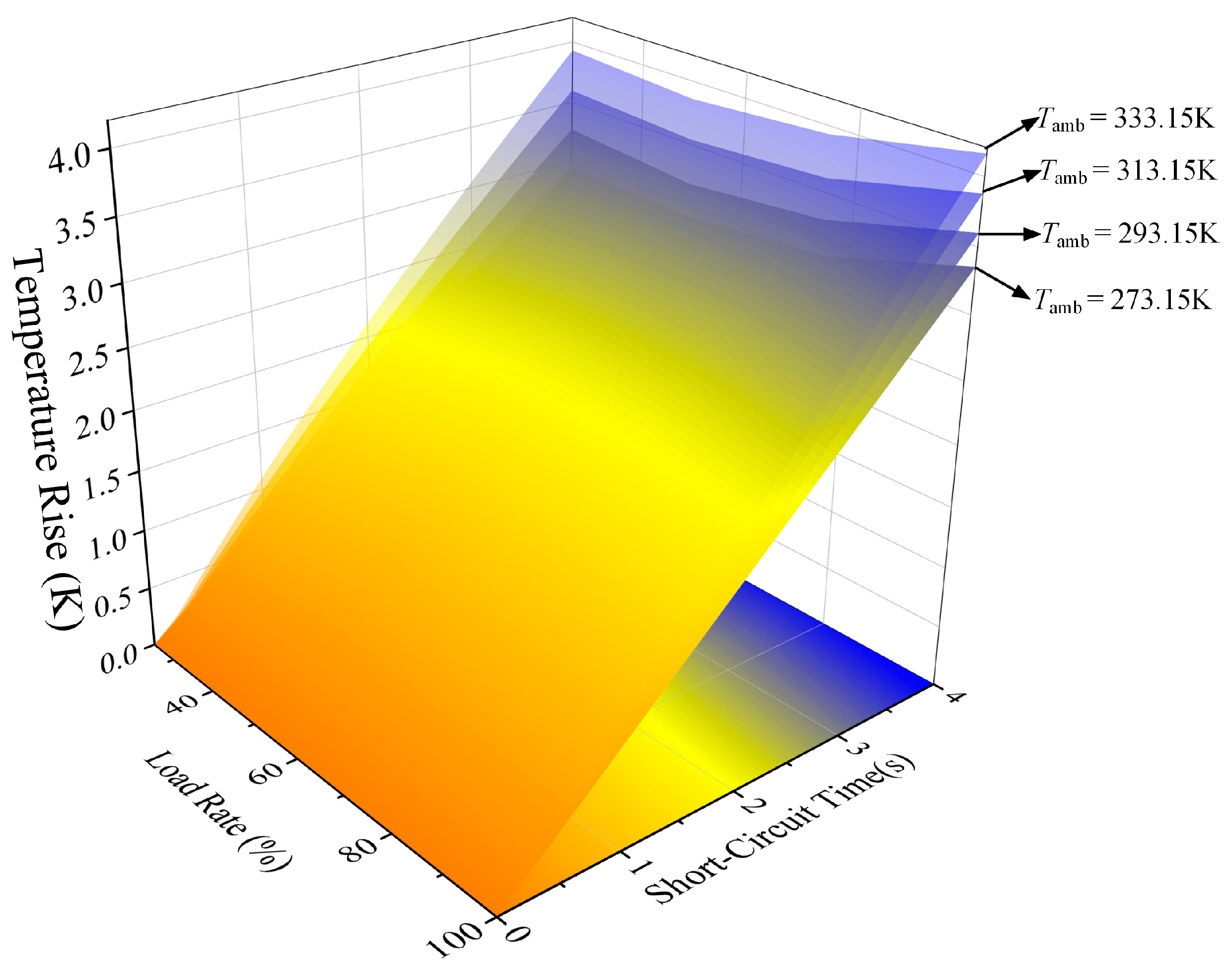
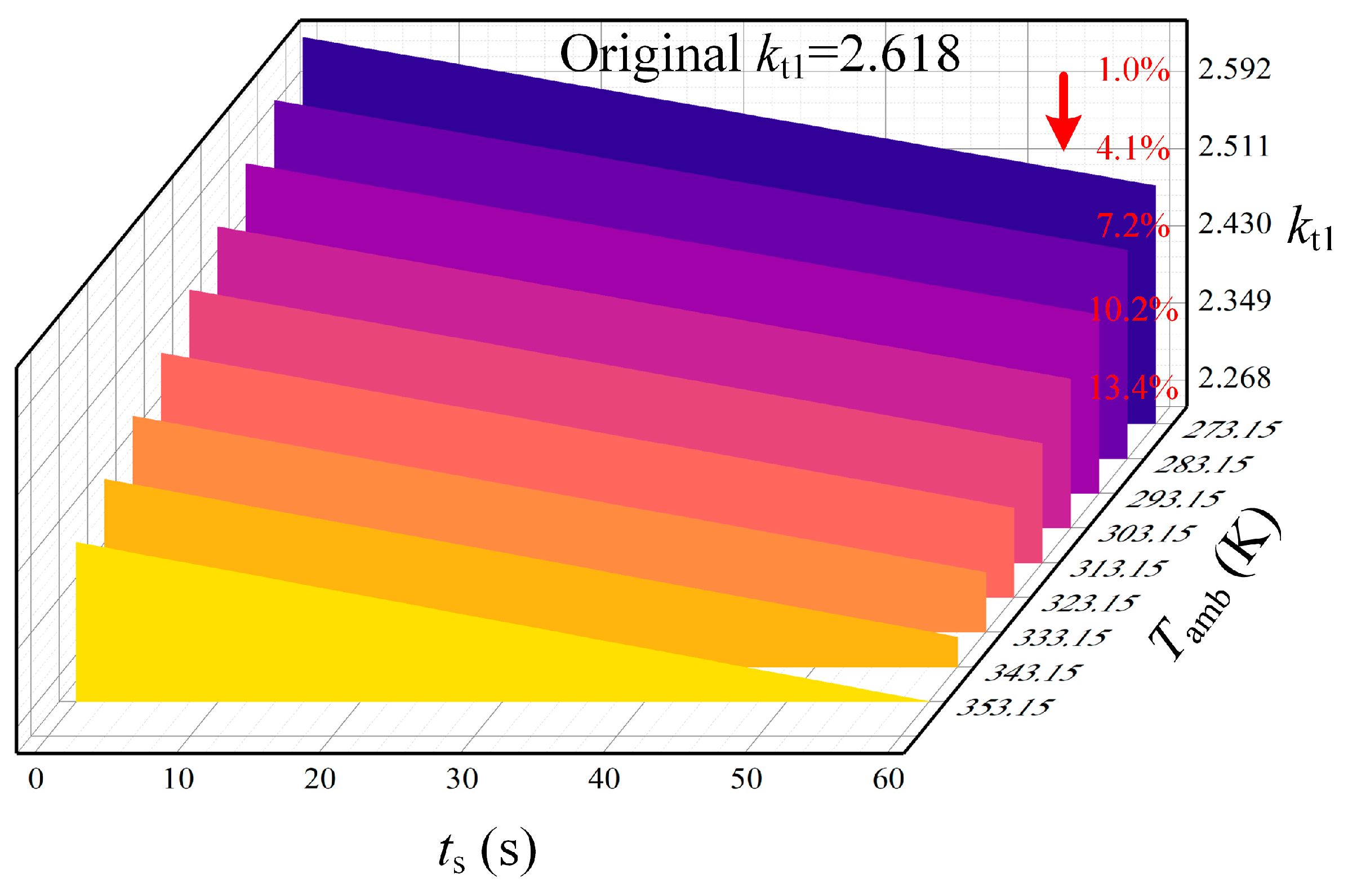
4.2. Transformer Heat-Flow Transient Field Calculations and Winding Hot Spot Temperature Fitting

For the transient calculation model, the excitation employed comprises the copper losses and core losses of the transformer during the short-circuit process. Due to the extremely short duration of the short-circuit process and the presence of external insulation in the windings, temperature changes in the windings cannot be promptly transmitted to the temperature measurement fiber optics. Therefore, the short-circuit temperature rise is challenging to directly measure through experiments. To address this, the excitation source of the previously validated steady-state model is modified. The copper losses from the short-circuit current in the transformer windings and the core losses are used as excitation. The boundary conditions remain the same and can be used to approximately calculate the transient temperature rise in the windings.

In this study, transient temperature rises in the transformer windings are calculated for load rates of 25%, 50%, 75%, and 100%, ambient temperatures of 273.15 K, 293.15 K, 313.15 K, and 333.15 K, and short-circuit times ranging from 0 s to 4 s. The computational results are presented as follows: at a short-circuit time of 4 s, the variation in the hot spot temperature with ambient temperature at different load rates; at the same short-circuit time of 4 s, the variation in the hot spot temperature with load rates at different ambient temperatures; and the variation in the short-circuit temperature rise with short-circuit times at different short-circuit load rates and ambient temperatures. The corresponding figures are shown below.

As can be seen from Figure 10 and Figure 11 above, the transformer winding hot spot temperature and load rate can be considered to be approximately quadratic, while the ambient temperature and short-circuit time are approximately primary. Therefore, according to the multicollinearity theory, the transformer winding hot spot temperature (T_h), load rate (L_r), ambient temperature (T_amb), and short-circuit time (t_s) are fitted by the nonlinear least squares (nlinfit) method [26], and the objective functions are as follows:

$$\begin{array}{c}T\mathrm{h}=\left(p_1\cdot L_{\mathrm{r}}^2+p_2\cdot L_{\mathrm{r}}+p_3\right)\\ \times \left(p_4\cdot T_{\mathrm{amb}}+p_5\right)\times (p_6\cdot t_{\mathrm{s}}+p_7)-p_8\end{array}$$

(21)

The fitted equation to obtain the transformer winding hot spot temperature versus the load rate, ambient temperature, and short-circuit time is given as follows:

$$\begin{array}{c}{T}_{\mathrm{h}}=\left(0.0178\cdot L_{\mathrm{r}}^2+0.5003\cdot L_{\mathrm{r}}^2+3549.6\right)\\ \times \left(0.0077\cdot T_{\mathrm{amb}}+8.4843\right)\\ \times (2.7546\cdot {10}^{-5}\cdot t_{\mathrm{s}}+0.0349)-776.55\end{array}$$

(22)

The root mean square (RMS) error image of this fit is shown below.

It can be seen that the fitting function has a small error in Figure 12, which is within the engineering permissible range, thus allowing verification of the accuracy of the fitting function.

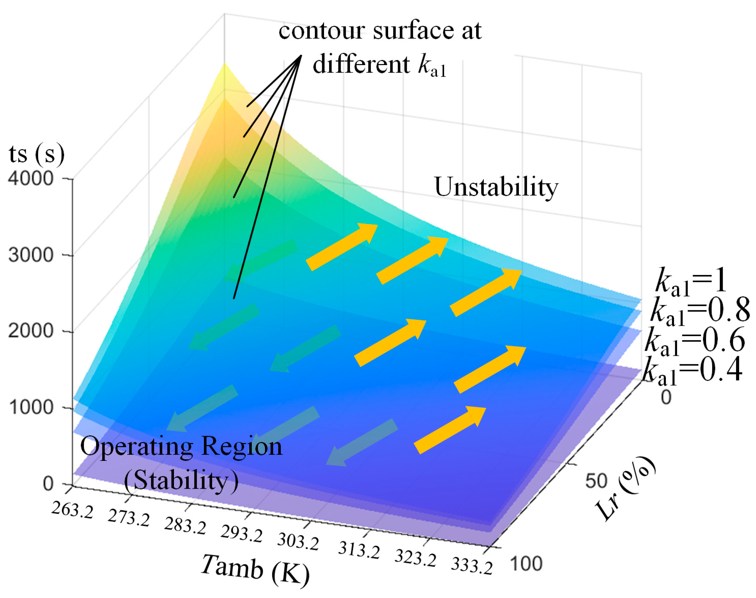
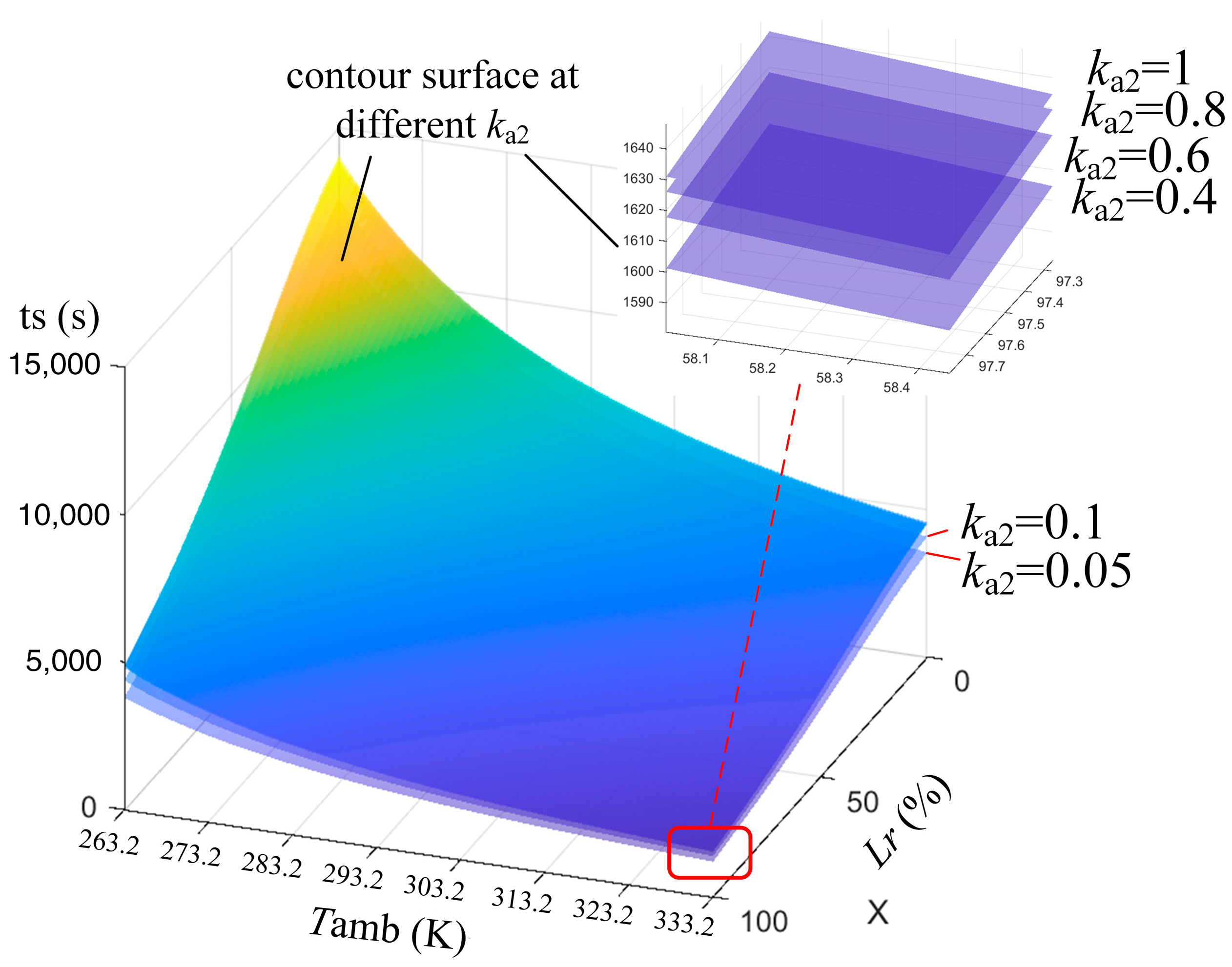
4.3. Calculation and Analysis of Mechanical Stability Margins of Power Transformer Windings Taking into Account Temperature Field

The above transformer winding mechanical stability verification did not consider the influence of temperature on the transformer winding material parameters. In fact, the transformer copper winding yield strength and modulus of elasticity change with the temperature. The relationship between the two parameters and the temperature can be approximated as a primary function as shown below.

$$\begin{array}{c}{R}_{\mathrm{p}0.2}=-0.18T+174.42\\ E=-0.04993T+130\end{array}$$

(23)

The unit of R_p0.2 is MPa, and the unit of E is GPa.

The mechanical stability margin of transformer winding characterized by different stresses is defined as the ratio of the stress to its critical value, in which the mechanical stability margin of the mean hoop compressive stress is relatively the lowest, and the value of the margin is calculated as follows:

$$k_{\mathrm{t}1}={\displaystyle \frac{0.35R_{\mathrm{p}0.2}}{{\sigma }_{\mathrm{t}1}}}=2.618$$

(24)

It can be seen that the margin should not be less than 1, if it is less than 1, then the transformer windings will probably lose mechanical stability. It is useful to analyze this margin by considering the temperature characteristics of the yield strength, and it is clear that when the temperature changes, the margin value will change accordingly. Considering the more severe case, the transformer is operated at a 100% load rate, and the variation in the margin value with short-circuit time and ambient temperature is shown in Figure 13.

The right side of the z-axis in the figure above shows the value of the mean hoop compressive stress margin kt1, and the percentage on the left side is the percentage of deviation between this margin value and the original margin value without considering the effect of temperature. It can be seen that as the ambient temperature of the transformer rises and the short-circuit time increases, the margin will decrease, and in extreme cases, such as at high load rates, high ambient temperatures, and failure to remove short-circuit faults in time, the mechanical stability margin will be significantly reduced, and if there is insufficient margin in the transformer design or if the strength of the transformer winding materials deteriorates, the likelihood of mechanical instability of the transformer will be increased.

To further evaluate the mechanical stability of transformer windings under varying temperatures, the analysis approach is outlined as follows: Initially, based on the computed stress values characterizing the mechanical stability of the transformer windings, critical values for R_p0.2 and E are calculated. Subsequently, considering the relationship between R_p0.2 and E with temperature, the degradation of the yield strength or elasticity modulus of the winding material is assessed. The minimum stress margin is then calculated, taking into account the actual critical temperature value related to the material degradation level. Finally, based on the obtained critical hot spot temperature, using the fitting function relating the hot spot temperature to ambient temperature, load rate, and short-circuit time, corresponding contour surfaces are determined. The region above the contour surfaces represents the area where the transformer is subjected to three-phase short-circuit impact and becomes unstable. Below the contour surfaces lies the region where the transformer operates with sufficient margin for mechanical stability, defined as the operating domain. A larger operating domain indicates a greater safety margin for stable transformer operation.

Regarding the verification item related to yield strength, let the degree of yield strength degradation be represented as k_a1. Assuming that the yield strength of the degraded copper winding changes with temperature in a manner consistent with the undegraded state, the actual yield strength of the transformer winding after degradation can be expressed as R_p0.2 = k_a1·(−0.18 T + 174.42). The actual degree of degradation is influenced by factors such as the operational lifespan of the transformer, the occurrences of short-circuit impacts during service, and maintenance conditions, and is difficult to precisely determine. As the average circumferential stress provides the minimum margin, this stress value is used to calculate the actual critical temperature for the hot spot, which is as follows:

$$T{\mathrm{h}}_{\mathrm{cr}}={\displaystyle \frac{174.42-\left(0.35\cdot k_{a1}\right)/21.43}{0.18}}$$

(25)

Taking the degree of degradation as 1 (not degraded), 0.8, 0.6, and 0.4, respectively, the operating domain is calculated as shown in Figure 14.

From the above figure, it is evident that the relationship among the mechanical stability of transformer windings and load levels, ambient temperature, and short-circuit times is affected by the consideration of yield strength degradation. With an increase in the degree of degradation, the operational domain of the mechanical stability of the transformer windings progressively diminishes. This implies that the margin of mechanical stability considering temperature conditions decreases continuously. Once the degradation reaches a certain threshold, the transformer experiences operating conditions beyond its operational domain, leading to mechanical instability of the transformer windings.

Subsequently, considering the condition of modulus of elasticity, let the degradation coefficient of the modulus of elasticity be denoted as k_a2. Assuming that the elastic modulus of the copper windings after degradation changes with temperature in a manner consistent with the undegraded state, the actual elastic modulus of the transformer windings after degradation can be expressed as E = k_a2·(−0.04993 T + 130). By relating the average circumferential stress to the free buckling limit stress, the actual critical temperature for the hot spot can be determined as follows:

$$T{\mathrm{h}}_{\mathrm{cr}}^{\prime }={\displaystyle \frac{130,000-\left(21.43\cdot 4\right)/{\left(\frac{86.5}{360.25}\right)}^2\cdot k_{a2}}{49.93}}$$

(26)

Considering the small coefficient of proportionality between elastic modulus and temperature, the operating domains were calculated as shown below by taking the degradation degree as 1 (undegraded), 0.8, 0.6, 0.4, 0.1, and 0.05, respectively, in order to show the variation in the operating domains with the degradation degree more clearly.

From Figure 15, it is evident that compared to the scenario considering yield strength, when considering the condition of modulus of elasticity, the operational domain is larger. Furthermore, the intervals between the operational domains of the windings under the six degrees of degradation shown in the figure are very small. This is because under the condition of modulus of elasticity, the mechanical stability margin of the windings is larger, and the impact of degradation on its stability is relatively minor. Therefore, the transformer windings exhibit a strong ability to withstand significant degradation in stiffness.

5. Conclusions

This paper analyzed parameters such as transformer operating load rate, ambient temperature, and short-circuit time, considering the impact of degradation in yield strength and modulus of elasticity parameters. It revealed the extent and patterns of how the mechanical stability of transformer windings is influenced by temperature, providing a method for analyzing the mechanical stability margin of transformer windings that accounts for the temperature field effect. This method assists in more reasonably verifying the mechanical stability of windings in transformers based on actual operating conditions and material parameter degradation.

The paper established a short-circuit current calculation model to provide accurate and reasonable excitation. A 3D electromagnetic force finite element model was developed using an SFZ-40000/110 oil-immersed transformer to calculate the radial and axial electromagnetic forces acting on the windings. The electromagnetic force results were then utilized in a numerical computation for the mechanical stability verification of the windings. Additionally, a 3D electromagnetic–thermal finite element model was established to compute the steady-state temperature field, which was validated through transformer temperature rise tests. Using this validated model as the initial state, transient temperature field calculations were performed. Finally, employing multicollinearity theory and least squares fitting, an expression was derived to show how the hot spot temperature of the transformer windings varies with load rate, ambient temperature, and short-circuit time. This expression was used to analyze changes in the mechanical stability margin of the windings under varying material parameter degradation levels, determining the operational domain where the transformer remains stable under three-phase short-circuit impacts.

The proposed method offers an effective approach for analyzing changes in the mechanical stability margin of transformer windings under temperature influences, providing valuable insights for transformer design and offering a clear practical utility for analyzing the mechanical stability of transformers in operation.

In view of some limitations found in the current research and areas where further progress can be made, the following work needs to be carried out in the future:

• Design more experimental conditions to verify the model more comprehensively and universally. Specifically, increase more load rates and carry out related experiments at various ambient temperatures.
• Design a reasonable method for a transient temperature rise test of transformer windings. Due to the short transient time and small transient temperature change, there is no low-cost and high-precision method to measure the transient temperature rise in transformer windings. This is an urgent problem to be solved to study the influence of transformer short-circuit temperature rise on the mechanical stability of transformer windings.
• Accurately measure the influence of temperature on the yield strength and elastic modulus of transformer windings. Subject to the experimental conditions of material mechanics, the relationship among winding yield strength, elastic modulus, and temperature used in this paper refers to the existing articles. In the future, targeted measurements should be carried out for the target transformer used to more accurately evaluate the influence of temperature on winding mechanical stability.

References

1. Zhang, B.; Yan, N.; Ma, S.; Wang, H. Buckling Strength Analysis of Transformer Windings Based on Electromagnetic Thermal Structural Coupling Method. IEEE Trans. Appl. Supercond. 2019, 29, 1–4. [Google Scholar] [CrossRef]
2. Meško, N.; Ćućić, B.; Žarko, D. Short-Circuit Stress Calculation in Oval Windings. Procedia Eng. 2017, 202, 319–326. [Google Scholar] [CrossRef]
3. Wang, J. Research on Anti-Short Circuit Ability of Power Transformer Considering Heat Accumulation Effect. Master’s Thesis, Shenyang University of Technology, Shenyang, China, 2023. [Google Scholar]
4. Ou, Q. Investigation on Evaluation of Mechanical Damage and Cumulative Effect for Power Transformer Windings Under Short Circuit Impact. Ph.D. Thesis, Hunan University, Changsha, China, 2023. [Google Scholar]
5. GB 1094.5-2008; General Administration of Quality Supervision, Inspection and Quarantine of the People’s Republic of China, Standardization Administration of the People’s Pepublic of China. Power Transformer-Part 5: Ability to Withstand Short Circuit. China Standard Press: Beijing, China, 2008.
6. IEC 60076-5; Power Transformer-Part 5: Ability to Withstand Short Circuit. International Electrotechnical Commission: Geneva, Switzerland, 2006.
7. Li, K. Study on Calibration Models and Evaluation Technology for Short Circuit Withstand Ability of Power Transformer. Master’s Thesis, Nanjing University of Aeronautics and Astronautics, Nanjing, China, 2016. [Google Scholar]
8. Ou, Q.; Luo, L.; Li, Y.; Li, Y.; Xiang, J. Buckling Strength Investigation for Power Transformer Winding Under Short Circuit Impact Considering Manufacture and Operation. IEEE Access 2023, 11, 7850–7859. [Google Scholar] [CrossRef]
9. Bakshi, A.; Kulkarni, S.V. Analysis of Buckling Strength of Inner Windings in Transformers Under Radial Short-Circuit Forces. IEEE Trans. Power Deliv. 2014, 29, 241–245. [Google Scholar] [CrossRef]
10. Cotas, C.; Santos, R.J.; Gonçalves, N.D.; Quintela, M.; Couto, S.; Campelo, H.; Dias, M.M.; Lopes, J.C.B. Numerical Study of Transient Flow Dynamics in a Core-Type Transformer Windings. Electr. Power Syst. Res. 2020, 187, 106423. [Google Scholar] [CrossRef]
11. Zhang, Y.; Ho, S.-L.; Fu, W.; Yang, X.; Wu, H. Numerical Study on Natural Convective Heat Transfer of Nanofluids in Disc-Type Transformer Windings. IEEE Access 2019, 7, 51267–51275. [Google Scholar] [CrossRef]
12. Zhang, X.; Wang, Z.; Liu, Q. Prediction of Pressure Drop and Flow Distribution in Disc-Type Transformer Windings in an OD Cooling Mode. IEEE Trans. Power Deliv. 2017, 32, 1655–1664. [Google Scholar] [CrossRef]
13. Tsili, M.A.; Amoiralis, E.I.; Kladas, A.G.; Souflaris, A.T. Power Transformer Thermal Analysis by Using an Advanced Coupled 3D Heat Transfer and Fluid Flow FEM Model. Int. J. Therm. Sci. 2012, 53, 188–201. [Google Scholar] [CrossRef]
14. Xiao, J.; Zhang, Z.; Hao, Y.; Zhao, H.; Liu, X. Method for Measuring Thermal Flow Field Distribution in Oil-Immersed Transformer Using Dynamic Heat Transfer Coefficient. IEEE Trans. Instrum. Meas. 2024, 73, 1–11. [Google Scholar] [CrossRef]
15. Zhao, H.; Zhang, Z.; Yang, Y.; Xiao, J.; Chen, J. A Dynamic Monitoring Method of Temperature Distribution for Cable Joints Based on Thermal Knowledge and Conditional Generative Adversarial Network. IEEE Trans. Instrum. Meas. 2023, 72, 1–14. [Google Scholar] [CrossRef]
16. Liu, G.; Rong, S.; Wu, W.; Wang, X.; Li, L. A Two-Dimensional Transient Fluid-Thermal Coupling Method for Temperature Rising Calculation of Transformer Winding Based on Finite Element Method. AIP Adv. 2020, 10, 035325. [Google Scholar] [CrossRef]
17. Liu, G.; Jin, Y.J.; Ma, Y.Q.; Sun, L.; Chi, C. 2-D transient temperature field simulation of oil-immersed transformer based on hybrid method. High Volt. Appar. 2019, 55, 82–89. [Google Scholar] [CrossRef]
18. Hayt, W.H.; Buck, J.A. Engineering Electromagnetics, 9th ed.; McGraw-Hill Education: New York, NY, USA, 2019. [Google Scholar]
19. Liu, F.; Li, D.; Wang, Y.; Li, Y.; Zhao, Z.; Yang, Q. Analysis of Magnetizing Process Using the Discharge Current of Capacitor by T-Ω Method. IEEE Trans. Appl. Supercond. 2016, 26, 1–4. [Google Scholar] [CrossRef]
20. Nagsarkar, T.K.; Sukhija, M.S. Power System Analysis; Oxford University Press: New Delhi, India, 2014. [Google Scholar]
21. Ma, J. Power System Analysis and Control Theory; John Wiley & Sons, Ltd.: Singapore, 2018. [Google Scholar]
22. Ceraolo, M.; Poli, D. Fundamentals of Electric Power Engineering; John Wiley & Sons, Inc.: Hoboken, NJ, USA, 2014. [Google Scholar]
23. Kebriti, R.; Hossieni, S.M.H. 3D Modeling of Winding Hot Spot Temperature in Oil-Immersed Transformers. Electr. Eng. 2022, 104, 3325–3338. [Google Scholar] [CrossRef]
24. Bergman, T.L.; Lavine, A.; Incropera, F.P.; DeWitt, D.P. Fundamentals of Heat and Mass Transfer; Wiley: Hoboken, NJ, USA, 2018. [Google Scholar]
25. Li, H.; Liu, Y.; Wang, J.; Zhang, W.; Sui, Y.; Fan, X. Analysis and test verification of dynamic thermal model of oil-immersed distribution transformer. Proc. CSEE 2023, 43, 389–399. [Google Scholar] [CrossRef]
26. Wang, L.; Li, X.; Xu, M.; Guo, Z.; Wang, B. Study on optimization model control method of light and temperature coordination of greenhouse crops with benefit priority. Comput. Electron. Agric. 2023, 210, 107892. [Google Scholar] [CrossRef]
Figure 1. Transformer winding current calculation model.
Energies 18 01374 g001
Figure 2. (a) Low-voltage winding steady-state current; (b) high voltage winding steady-state current; (c) low-voltage winding short-circuit current; (d) high voltage winding short-circuit current.
Energies 18 01374 g002
Figure 3. Transformer finite element model.
Energies 18 01374 g003
Figure 4. (a) Winding radial force and (b) winding axial force at 0.01 s.
Energies 18 01374 g004
Figure 5. Winding copper loss.
Energies 18 01374 g005
Figure 6. Core loss distribution.
Energies 18 01374 g006
Figure 7. Steady-state temperature field of windings at (a) 50% load rate; (b) 75% load rate; (c) 100% load rate.
Energies 18 01374 g007
Figure 8. Schematic layout of test probes and data collection.
Energies 18 01374 g008
Figure 9. Transformer hot spot temperature variation under different load rate tests.
Energies 18 01374 g009
Figure 10. Schematic diagram of (a) winding hot spot temperature variation with load rate and (b) winding hot spot temperature variation with ambient temperature.
Energies 18 01374 g010
Figure 11. Schematic diagram of winding hot spot temperature variation with short-circuit time.
Energies 18 01374 g011
Figure 12. Fitting the root mean square error image.
Energies 18 01374 g012
Figure 13. Image of kt1 variation with short-circuit time and ambient temperature.
Energies 18 01374 g013
Figure 14. Operating domain of mechanical stability of transformer windings.
Energies 18 01374 g014
Figure 15. Operating domain of mechanical stability of transformer windings taking into account modulus of elasticity variation with temperature characteristics.
Energies 18 01374 g015