Enhanced Models for Wind, Solar Power Generation, and Battery Energy Storage Systems Considering Power Electronic Converter Precise Efficiency Behavior

Abstract

The large-scale integration of wind, solar, and battery energy storage is a key feature of the new power system based on renewable energy sources. The optimization results of wind turbine (WT)–photovoltaic (PV)–battery energy storage (BES) hybrid energy systems (HESs) can influence the economic performance and stability of the electric power system (EPS). However, most existing studies have overlooked the effect of power electronic converter (PEC) efficiency on capacity configuration optimization, leading to a significant difference between theoretical optimal and actual results. This paper introduces an accurate efficiency model applicable to different types of PECs, and establishes an enhanced mathematical model along with constraint conditions for WT–PV–BES–grid–load systems, based on precise converter efficiency models. In two typical application scenarios, the capacity configurations of WT–PV–BES are optimized with optimal cost as the objective function. The different configuration results among ignoring PEC loss, using fixed PEC efficiency models, and using accurate PEC efficiency models are compared. The results show that in the DC system, the total efficiency of the system with the precise converter efficiency model is approximately 96.63%, and the cost increases by CNY 49,420, about 8.56%, compared to the system with 100% efficiency. In the AC system, the total efficiency with the precise converter efficiency model is approximately 97.64%, and the cost increases by CNY 4517, about 2.02%, compared to the system with 100% efficiency. The analysis clearly reveals that the lack of an accurate efficiency model for PECs will greatly affect the precision and effectiveness of configuration optimization.

1. Introduction

In recent years, under the background of low carbon targets and the rapid upgrading of wind, solar, and storage industry technologies, HESs, including WTs, PV systems, and energy storage systems (ESSs), have become the mainstream trend in the future development of new EPSs [1,2,3]. The optimization of WTs, PV systems, and ESS capacity configuration has been extensively studied and widely discussed in various HESs, microgrids, and EPSs. These new EPSs integrate multiple energy sources to improve system reliability and efficiency while minimizing carbon emissions.

However, existing studies often overlook a key factor in system capacity configuration optimization: the dynamic characteristics of the power electronics converter (PEC) efficiency. Converters are critical devices for integrating WT, PV, BES, and other energy sources into the grid, and their efficiency varies significantly with operating conditions, as shown in Figure 1. Due to the lack of an accurate PEC efficiency model, optimizing the capacity configuration of these systems remains a complex challenge.

Studies often do not fully consider the influence of these converters, especially regarding their energy conversion efficiency. Most of the existing research directly provides fixed values as the converter conversion efficiency. For instance, the fixed efficiency of the inverter between the DC and AC bus is given in refs. [4,5,6,7,8,9,10,11]. The fixed efficiency of the converter connected to WT, PV, and BES systems is considered in refs. [6,11,12], refs. [11,13,14,15,16,17], and ref. [12], respectively. These studies directly provide values for converter efficiency but do not provide the basis for these values, which exhibits strong subjectivity. Furthermore, some studies only consider the efficiency of certain converters in the system, which can lead to inaccurate configuration optimization results. For example, ref. [4] discusses the prospects of utilizing hydrogen for energy storage, offering insights into the configuration of current and future hybrid energy systems. Ref. [5] proposes an integrated sustainable energy system composed of PV arrays, WTs, concentrated solar power stations, BES, electric heaters, and inverters, obtaining the optimal configuration and sizing of energy generation and storage devices. However, both studies use a fixed efficiency value of 95% for converters. Ref. [8] adopts a 92% efficiency model for grid-connected inverters. Ref. [11] considers a 95% efficiency model for WT converters. Ref. [16] takes a 95% efficiency model for PV converters. Ref. [12] assumes a 95% efficiency model for various types of converters. Furthermore, several studies have even overlooked the influence of converter efficiency on system configuration optimization. In refs. [18,19], losses generated by the converter during the energy conversion process in the WT–PV–BES hybrid energy system are overlooked. Apparently, the incomplete efficiency model of PECs mentioned above will significantly affect the accuracy of the configuration results.

The existing research on power system configuration optimization primarily involves the following steps: the construction of energy generation models, the design of objective functions and assessment metrics, and optimization using intelligent algorithms. For different power systems, appropriate comprehensive evaluation indicators and optimization algorithms should be selected. The common economic evaluation indicators include levelized cost of energy (LCOE) [5,6,13,14,15,16,20], cost of energy (COE) [7,8,9,19], net present value (NPV) [14,21], and net present cost (NPC) [17,20]. The reliability evaluation indicators include loss of power supply probability (LPSP) [5,6,7,8,9,17,19,21], etc. The ecological evaluation indicators include total greenhouse gas emission cost [8,17,22], etc. Furthermore, classical heuristic algorithms, such as genetic algorithm, particle swarm optimization, grey wolf algorithm, and differential evolution algorithm, are commonly applied to solve the capacity configuration optimization problems of simple EPSs [9,15]. However, in complex EPSs, these algorithms tend to get trapped in local optimal solutions, and the changes in algorithm parameters significantly impact the optimization results, and the convergence speed of the algorithm is unstable. Therefore, some improved algorithms have been proposed and applied in large EPS optimization research. The improved whale algorithm [23] and the modified manta ray foraging algorithm [24] exhibited better global search capabilities. The improved grey wolf algorithm [25] has better adaptability and does not need to adjust many parameters. The improved clustering algorithm [26] has higher accuracy. The selection of appropriate algorithms for HES configuration optimization plays a vital role in ensuring the low-cost operation of the EPS.

Therefore, this paper analyzes the performance characteristics and main loss sources of different PECs from the PEC topology and working mechanism, proposes an accurate efficiency model applicable to different PECs, and establishes the mathematical models and constraints conditions for WT–PV–BES–grid–load. Meanwhile, with minimizing cost as the objective function, accounting for the investment costs and the operation and maintenance costs of the power sources and power converters, WT–PV–BES configurations are optimized using particle swarm optimization algorithms in typical AC and DC grid application scenarios. Finally, the significant advantages of the PEC accurate efficiency model are demonstrated through a comparative analysis of the configuration results under the fixed PEC efficiency model and the accurate PEC efficiency model. The application of accurate PEC models makes the capacity configuration results of EPSs more reasonable. This paper provides important references and applications for future research on optimizing EPS configurations.

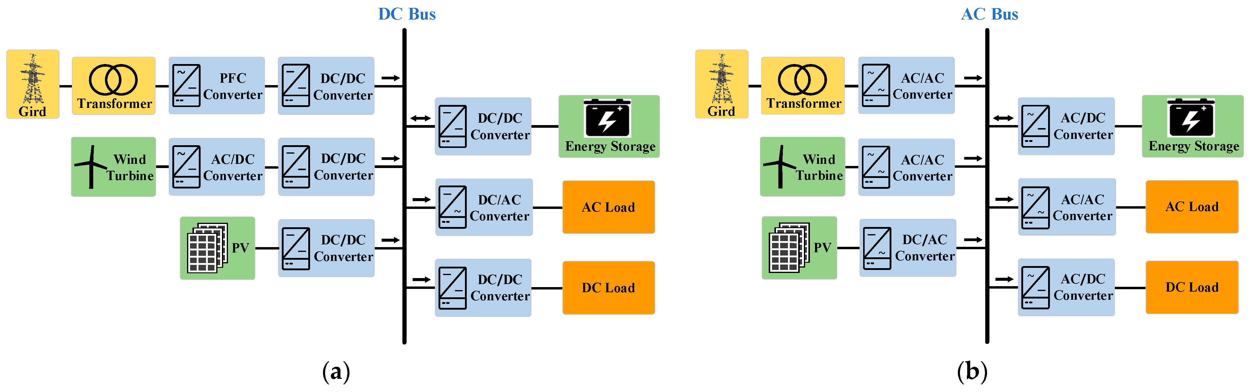
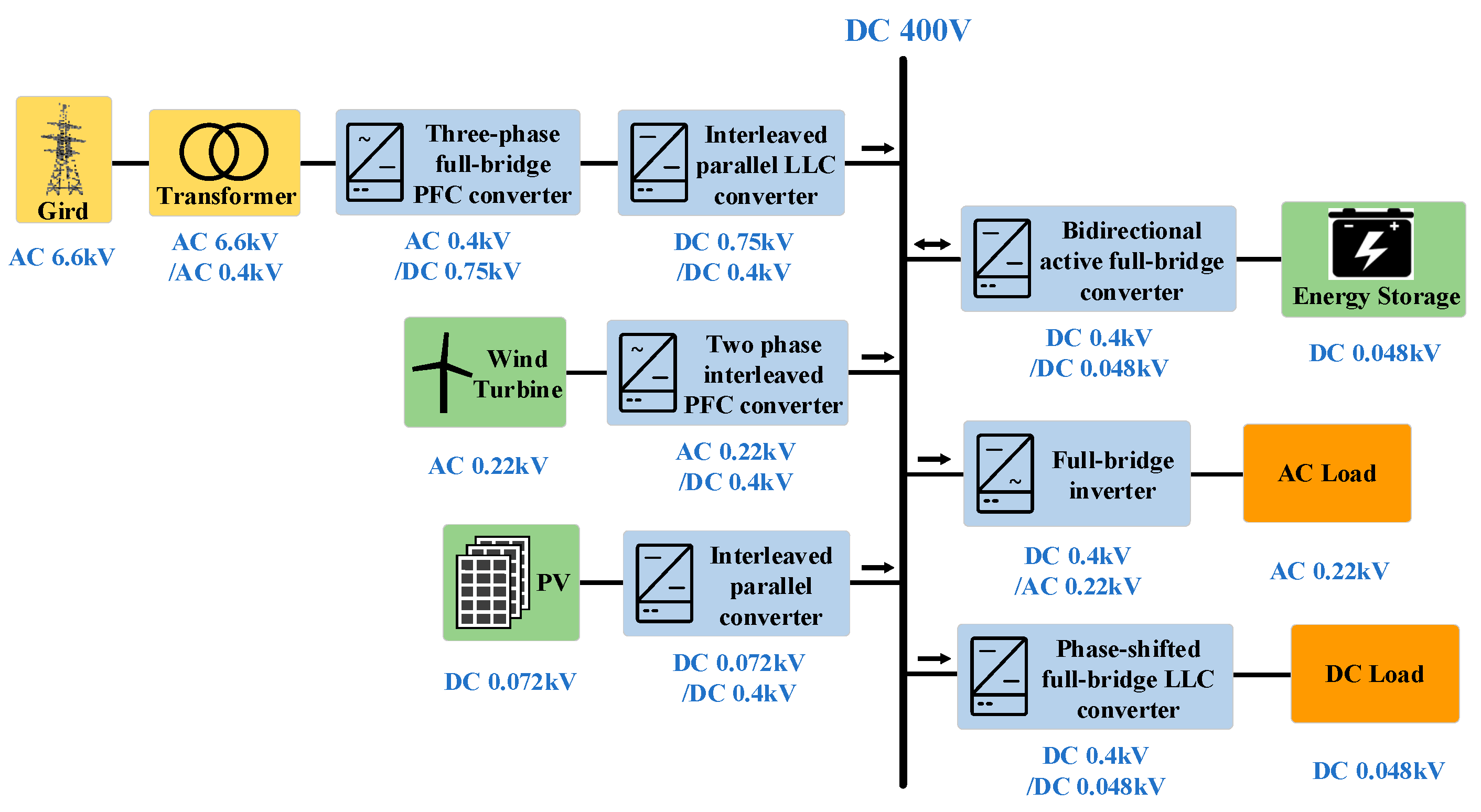
2. AC/DC Power System Structures and Efficiency Model of PECs

PECs are the key devices that connect different power sources and AC/DC loads. Usually, as seen in Figure 2a, in a DC power system, PV systems are interfaced with the bus via DC/DC converters. The WT system links to the bus via a cascade of AC/DC and DC/DC converters. The battery energy storage system (BESS) links to the bus via bidirectional DC/DC converters. The power grid links to the bus via power factor correction (PFC) converters and DC/DC converters. Loads will obtain electricity from the bus after single-stage or multi-stage conversion through DC/DC converters or DC/AC converters. In Figure 2b, AC power systems are similar to DC power systems, except for the type of PECs. The PV system, BESS, and DC loads link to the bus through DC/AC converters. The power grid, WT system, and AC loads link to the bus through AC/AC converters [27].

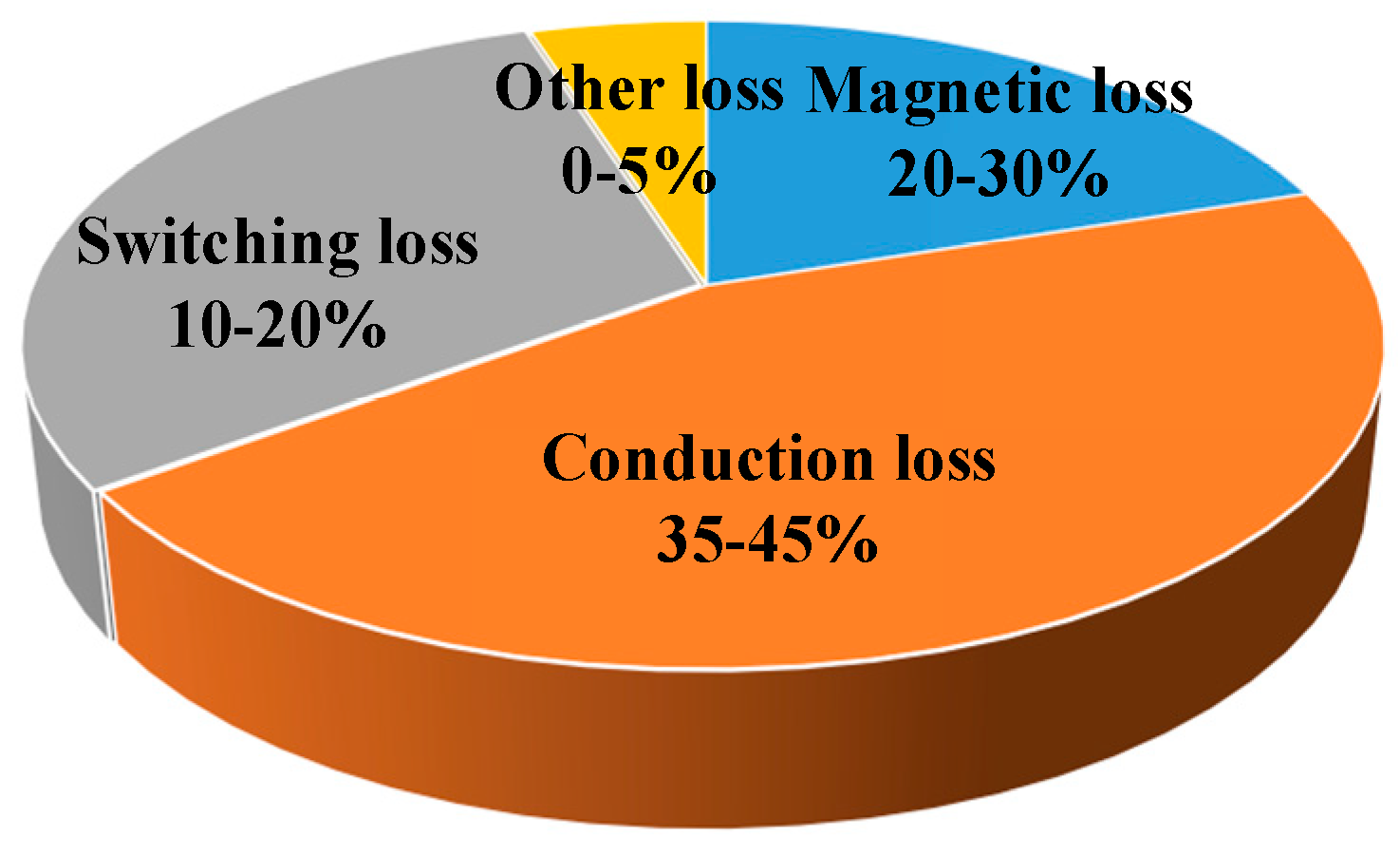
2.1. Converter Loss Analysis

PECs are generally composed of switching devices (such as Infineon Technologies AG (Munich, Germany) MOSFET and IGBT), diodes, capacitors, inductors, and other electronic devices. Losses will inevitably be produced during the operation of PECs. The main sources of losses are shown in Figure 3: ① Conduction loss: due to internal resistance or terminal voltage of some devices, losses are generated when a current flows through them. ② Switching loss: during the actual switching process of switching devices, the current and the voltage applied to its terminals will not suddenly become zero but gradually decrease to zero, resulting in switching losses. These losses are dependent on the switching frequency, switching speed, and characteristics of the switching devices. ③ Magnetic loss: some losses are generated by the hysteresis effect of magnetic devices in a periodically changing magnetic field. Other losses are caused by the induced currents flowing through the internal resistance of magnetic devices. ④ Other losses: including line losses, control circuit losses, etc. [28,29].

Specifically, the total losses $P_{\mathrm{loss}}(t)$ are shown in Equations (1) and (2) [30]:

$$P_{\mathrm{loss}}(t)=P_{\mathrm{loss}}^{L-\mathrm{copper}}(t)+P_{\mathrm{loss}}^{L-\mathrm{core}}(t)+P_{\mathrm{loss}}^{S-\mathrm{conduction}}(t)+P_{\mathrm{loss}}^{S-\mathrm{switch}}(t)+P_{\mathrm{loss}}^{D-\mathrm{conduction}}(t)+P_{\mathrm{loss}}^C(t)+P_{\mathrm{loss}}^{\mathrm{other}}(t)$$

(1)

where $P_{\mathrm{loss}}^{L-\mathrm{copper}}(t)$ is the inductor copper loss, $P_{\mathrm{loss}}^{L-\mathrm{core}}(t)$ is the inductor core loss, $P_{\mathrm{loss}}^{S-\mathrm{conduction}}(t)$ is the conduction loss of switch devices, $P_{\mathrm{loss}}^{S-\mathrm{switch}}(t)$ is the switching loss of switch devices, $P_{\mathrm{loss}}^{D-\mathrm{conduction}}(t)$ is the diode conduction loss, $P_{\mathrm{loss}}^C(t)$ represents the capacitor loss, $P_{\mathrm{loss}}^{\mathrm{other}}(t)$ represents the other loss [31,32]. Their expressions are as follows:

$$\{\begin{array}{l}{P}_{\mathrm{loss}}^{L-\mathrm{copper}}(t)={\displaystyle \frac{{\displaystyle {\int }_0^T{i}_L{(t)}^2\cdot R_{L}dt}}{T}}\\ P_{\mathrm{loss}}^{L-\mathrm{core}}(t)=k_{\mathrm{hl}}\cdot f\cdot {B_{\max }}^{{\alpha }_{\mathrm{hl}}}\\ P_{\mathrm{loss}}^{S-\mathrm{conduction}}(t)={\displaystyle \frac{{\displaystyle {\int }_0^T{i}_S{(t)}^2\cdot R_S}dt}{T}}\\ P_{\mathrm{loss}}^{S-\mathrm{switch}}(t)=f\cdot {\displaystyle \frac{I_{S(\max )}\cdot U_{S(\max )}\cdot \left(t_S^{\mathrm{rise}}+t_S^{\mathrm{fall}}\right)}{2}}\\ P_{\mathrm{loss}}^{D-\mathrm{conduction}}(t)={\displaystyle \frac{{\displaystyle {\int }_0^T{i}_D(t)\cdot U_D^{\mathrm{conduction}}dt}}{T}}\\ P_{\mathrm{loss}}^C(t)={\displaystyle \frac{{\displaystyle {\int }_0^T{i}_C{(t)}^2\cdot R_{C}dt}}{T}}\\ P_{\mathrm{loss}}^{\mathrm{other}}(t)=1\%P(t)\end{array}$$

(2)

where $P_{\mathrm{loss}}^{L-\mathrm{copper}}(t)$, $P_{\mathrm{loss}}^{S-\mathrm{conduction}}(t)$, $P_{\mathrm{loss}}^{S-\mathrm{switch}}(t)$, $P_{\mathrm{loss}}^{D-\mathrm{conduction}}(t)$, and $P_{\mathrm{loss}}^C(t)$ are determined by the parameters, switching frequency, and current and voltage of the device. $P_{\mathrm{loss}}^{L-\mathrm{core}}(t)$ is related to the electromagnetic coefficient. $P(t)$ is the operating power. $i_L(t)$, $i_S(t)$, $i_D(t)$, and $i_C(t)$ are the currents of inductors, switches, diodes, and capacitors, respectively. $R_L$, $R_S$, and $R_C$ are the internal resistances of inductors, switches, and capacitors, respectively. $t_S^{\mathrm{rise}}$ and $t_S^{\mathrm{fall}}$ are the current rise and fall times during the switching process of the switching device. $U_D^{\mathrm{conduction}}$ represents the voltage drop when diodes are conducting. $k_{\mathrm{hl}}$ is the hysteresis loss constant. $f$ represents the switching frequency. $B_{\max }$ represents maximum magnetic induction intensity, and ${\alpha }_{\mathrm{hl}}$ is the hysteresis loss exponent.

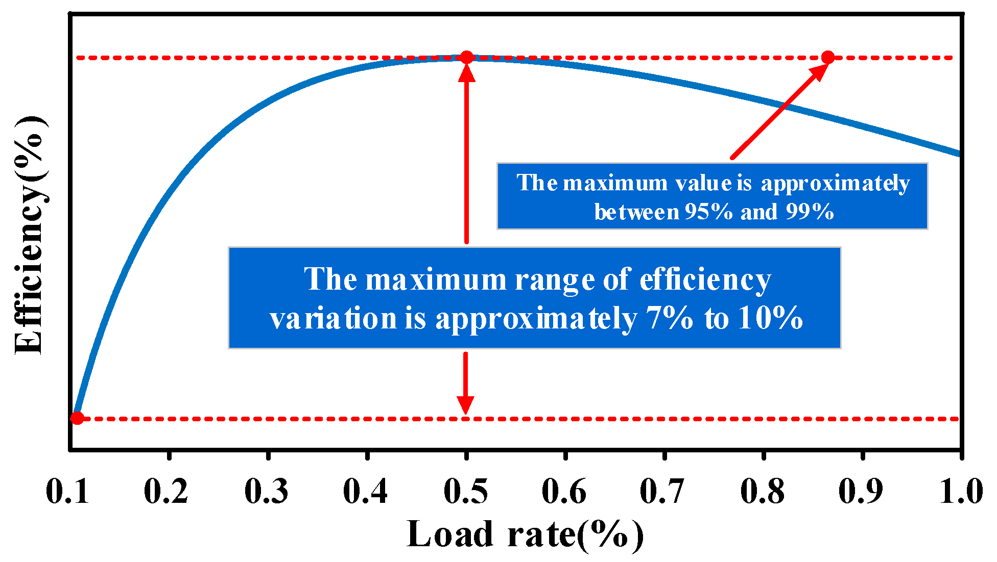
2.2. Converter Efficiency Model

Through loss analysis, the voltage and current of each device are determined by the specific circuit topology. The inductor current $i_L$ is affected by the input voltage $U_i$, output voltage $U_o$, inductor value $L$, load $R$, duty cycle $D$, and switching frequency $f$. In addition, the currents $i_S(t)$, $i_D(t)$, and $i_C(t)$ are linearly related to the inductor current $i_L(t)$. At the same time, the inductor current is generally linearly related to the input current $i_i(t)$. Therefore, $P_{\mathrm{loss}}(t)$ is a quadratic polynomial that can be represented by the operating power $P(t)$, as shown in Equation (3):

$$P_{\mathrm{loss}}(t)=aP{(t)}^2+bP(t)+c$$

(3)

The relationship among the converter efficiency $\eta (t)$, operating power $P(t)$, and power losses $P_{\mathrm{loss}}(t)$ is shown in Equation (4):

$$\eta (t)={\displaystyle \frac{P(t)-P_{\mathrm{loss}}(t)}{P(t)}}$$

(4)

The relationship between converter efficiency and operating power can be obtained in Equation (5) through Equations (3) and (4) as follows:

$$\eta (t)=aP(t)+{\displaystyle \frac{b}{P(t)}}+c$$

(5)

where the coefficients $a$, $b$, and $c$ are determined by the specific topology of the converter.

3. Enhanced AC/DC Power System Models

Existing power systems usually lack complete consideration of PEC efficiency. In this section, the precise efficiency model of PECs is applied to power supply equipment, grids, and loads. The specific improved power system models are described below.

3.1. Wind Turbine Model

Wind power generation converts kinetic energy into electricity. Output power is directly influenced by wind speed. If the wind speed falls below the cut-in speed, WTs fail to work. Once the wind speed surpasses the cut-in speed, by adjusting the electromagnetic torque of WTs, the wheel speed is matched with the wind speed to capture maximum energy. The output power remains stable when the wind speed exceeds the rated wind speed. During high wind speeds, WTs fail to work to avoid damage, as shown in Equations (6)–(8) [33]:

$$A{P}_{\mathrm{wt}}(t)=N_{\mathrm{p},1}\cdot {\eta }_{\mathrm{converter}}^{\mathrm{wt}}(t)\cdot P_{\mathrm{wt}}(t)$$

(6)

$${\eta }_{\mathrm{converter}}^{\mathrm{wt}}(t)=a_{\mathrm{wt}}\cdot P_{\mathrm{wt}}(t)+{\displaystyle \frac{b_{\mathrm{wt}}}{P_{\mathrm{wt}}(t)}}+c_{\mathrm{wt}}$$

(7)

$$P_{\mathrm{wt}}(t)=\{\begin{array}{ll}0,& 0\le v_{\mathrm{wt}}(t)<v_{\mathrm{wt}}^{\mathrm{ci}}\\ P_{\mathrm{wt}}^{\mathrm{rated}}\cdot {\displaystyle \frac{v_{\mathrm{wt}}(t)-v_{\mathrm{wt}}^{\mathrm{ci}}}{v_{\mathrm{wt}}^{\mathrm{rated}}-v_{\mathrm{wt}}^{\mathrm{ci}}}},& v_{\mathrm{wt}}^{\mathrm{ci}}\le v_{\mathrm{wt}}(t)<v_{\mathrm{wt}}^{\mathrm{rated}}\\ P_{\mathrm{wt}}^{\mathrm{rated}},& v_{\mathrm{wt}}^{\mathrm{rated}}\le v_{\mathrm{wt}}(t)\le v_{\mathrm{wt}}^{\mathrm{co}}\\ 0,& v_{\mathrm{wt}}(t)>v_{\mathrm{wt}}^{\mathrm{co}}\end{array}$$

(8)

The power constraint condition of WTs is shown in Equation (9):

$$0\le P_{\mathrm{wt}}(t)\le P_{\mathrm{wt}}^{\mathrm{rated}}$$

(9)

where $A{P}_{\mathrm{wt}}(t)$ represents the total power provided by the WTs to the bus in the hour $t$. $N_{p,1}$ is the number of WTs. ${\eta }_{\mathrm{converter}}^{\mathrm{wt}}(t)$ is the efficiency of each converter connected to the WTs in the hour $t$. $P_{\mathrm{wt}}(t)$ represents the output power of each WT in the hour $t$. $a_{\mathrm{wt}}$, $b_{\mathrm{wt}}$, and $c_{\mathrm{wt}}$ are the coefficients of the efficiency curve of the converter connected to WTs. $P_{\mathrm{wt}}^{\mathrm{rated}}$ represents each WT’s rated power. $v_{\mathrm{wt}}(t)$ represents real-time wind speed. $v_{\mathrm{wt}}^{\mathrm{ci}}$, $v_{\mathrm{wt}}^{\mathrm{rated}}$, and $v_{\mathrm{wt}}^{\mathrm{co}}$ represent the cut-in, rated, and cut-out wind speeds, respectively.

3.2. Photovoltaic System Model

Solar energy is converted into electrical energy through photovoltaic power generation. Output power is mainly affected by solar radiation intensity and environmental temperature. Because some parameters in the basic U-I curve derived from the equivalent circuit of PV panels are difficult to determine, this paper provides a simplified expression for the output power of PV panels [34,35], as shown in Equation (10) below:

$$\{\begin{array}{l}A{P}_{\mathrm{pv}}(t)=N_{\mathrm{p},2}\cdot {\eta }_{\mathrm{converter}}^{\mathrm{pv}}(t)\cdot P_{\mathrm{pv}}(t)\\ {\eta }_{\mathrm{converter}}^{\mathrm{pv}}(t)=a_{\mathrm{pv}}\cdot P_{\mathrm{pv}}(t)+{\displaystyle \frac{b_{\mathrm{pv}}}{P_{\mathrm{pv}}(t)}}+c_{\mathrm{pv}}\\ P_{\mathrm{pv}}(t)=P_{\mathrm{pv}}^{\mathrm{rated}}\cdot {\displaystyle \frac{I_{\mathrm{rsr}}(t)}{I_{\mathrm{ssr}}}}\cdot [1-k_{\mathrm{sat}}\cdot (T_{\mathrm{ra}}(t)-T_{\mathrm{sa}})]\end{array}$$

(10)

The constraint condition of PV panels is shown in Equation (11):

$$0\le P_{\mathrm{pv}}(t)\le P_{\mathrm{pv}}^{\mathrm{rated}}$$

(11)

where $A{P}_{\mathrm{pv}}(t)$ represents the total power provided by the PV system to the bus in the hour $t$. $N_{\mathrm{p},2}$ represents the number of PV panels. ${\eta }_{\mathrm{converter}}^{\mathrm{pv}}(t)$ represents the PV converter efficiency in hour $t$. $P_{\mathrm{pv}}(t)$ represents the output power of each PV panel in the hour $t$. $a_{\mathrm{pv}}$, $b_{\mathrm{pv}}$ and $c_{\mathrm{pv}}$ are coefficients of the efficiency curve of the PV converter. $P_{\mathrm{pv}}^{\mathrm{rated}}$ represents the rated power of each PV panel. $I_{\mathrm{rsr}}(t)$ represents real-time solar radiation intensity. $I_{\mathrm{ssr}}$ represents standard solar radiation intensity. $k_{\mathrm{sat}}$ represents standard environmental temperature coefficient. $T_{\mathrm{ra}}(t)$ represents real-time environmental temperature. $T_{\mathrm{sa}}$ is the standard environmental temperature.

3.3. Load Model

The loads generally include DC loads such as lighting and electronic equipment, and AC loads such as heating and cooling equipment, as shown in Equations (12)–(14) below:

$$\{\begin{array}{l}A{P}_{\mathrm{load}}(t)=A{P}_{\mathrm{load}}^{\mathrm{ac}}(t)+A{P}_{\mathrm{load}}^{\mathrm{dc}}(t)\\ A{P}_{\mathrm{load}}^{\mathrm{ac}}(t)={\displaystyle \frac{P_{\mathrm{load}}^{\mathrm{ac}}(t)}{{\eta }_{\mathrm{converter}}^{\mathrm{ac}}(t)}},A{P}_{\mathrm{load}}^{\mathrm{dc}}(t)={\displaystyle \frac{P_{\mathrm{load}}^{\mathrm{dc}}(t)}{{\eta }_{\mathrm{converter}}^{\mathrm{dc}}(t)}}\\ {\eta }_{\mathrm{converter}}^{\mathrm{ac}}(t)=a_{\mathrm{ac}}\cdot {\displaystyle \frac{P_{\mathrm{load}}^{\mathrm{ac}}(t)}{N_{\mathrm{c},5}}}+b_{\mathrm{ac}}\cdot {\displaystyle \frac{N_{\mathrm{c},5}}{P_{\mathrm{load}}^{\mathrm{ac}}(t)}}+c_{\mathrm{ac}}\\ {\eta }_{\mathrm{converter}}^{\mathrm{dc}}(t)=a_{\mathrm{dc}}\cdot {\displaystyle \frac{P_{\mathrm{load}}^{\mathrm{dc}}(t)}{N_{\mathrm{c},6}}}+b_{\mathrm{dc}}\cdot {\displaystyle \frac{N_{\mathrm{c},6}}{P_{\mathrm{load}}^{\mathrm{dc}}(t)}}+c_{\mathrm{dc}}\end{array}$$

(12)

$$N_{\mathrm{c},5}=\lceil \max P_{\mathrm{load}}^{\mathrm{ac}}(t)/P_{\mathrm{converter}}^{\mathrm{ac}-\mathrm{rated}}\rceil$$

(13)

$$N_{\mathrm{c},6}=\lceil \max P_{\mathrm{load}}^{\mathrm{dc}}(t)/P_{\mathrm{converter}}^{\mathrm{dc}-\mathrm{rated}}\rceil$$

(14)

where $A{P}_{\mathrm{load}}(t)$ represents the total power provided by the bus for the loads in the hour $t$, $A{P}_{\mathrm{load}}^{\mathrm{ac}}(t)$ and $A{P}_{\mathrm{load}}^{\mathrm{dc}}(t)$ are the total power provided by the bus for AC and DC loads in the hour $t$. $P_{\mathrm{load}}^{\mathrm{ac}}(t)$ and $P_{\mathrm{load}}^{\mathrm{dc}}(t)$ are the total power required by AC and DC loads in the hour $t$. ${\eta }_{\mathrm{converter}}^{\mathrm{ac}}(t)$ and ${\eta }_{\mathrm{converter}}^{\mathrm{dc}}(t)$ are, respectively, the efficiencies of the converters linked to the AC and DC loads in the hour $t$. $a_{\mathrm{ac}}$, $b_{\mathrm{ac}}$, and $c_{\mathrm{ac}}$ are coefficients of the efficiency curve of the converter connected to AC loads. $P_{\mathrm{converter}}^{\mathrm{ac}-\mathrm{rated}}$ and $P_{\mathrm{converter}}^{\mathrm{dc}-\mathrm{rated}}$ are, respectively, the rated power of the converters linked to the AC and DC loads. $a_{\mathrm{dc}}$, $b_{\mathrm{dc}}$ and $c_{\mathrm{dc}}$ are the coefficients of the efficiency curve of the converter connected to DC loads. $N_{\mathrm{c},5}$ and $N_{\mathrm{c},6}$ are, respectively, the number of converters linked to AC and DC loads. $N_{\mathrm{c},5}$ and $N_{\mathrm{c},6}$ are, respectively, calculated using a function whose value is the smallest integer greater than or equal to the numerical solution of Equations (13) and (14).

3.4. Battery Energy Storage System Model

The BESS can balance electrical energy supply and demand to maintain the continuous and stable operation of the EPS. The operation of the BESS involves continuous charging and discharging, represented by the state of charge (SOC) [36,37]. Without considering battery temperature and state of health (SOH), Equation (15) presents the discharging process as follows:

$$\{\begin{array}{l}A{P}_{\mathrm{es}}^{\mathrm{dis}}(t)=A{P}_{\mathrm{load}}(t)-A{P}_{\mathrm{pv}}(t)-A{P}_{\mathrm{wt}}(t)\\ {\eta }_{\mathrm{converter}}^{\mathrm{es}-\mathrm{dis}}(t)=a_{\mathrm{es}}\cdot {\displaystyle \frac{A{P}_{\mathrm{es}}^{\mathrm{dis}}(t)}{N_{\mathrm{p},3}}}+b_{\mathrm{es}}\cdot {\displaystyle \frac{N_{\mathrm{p},3}}{A{P}_{\mathrm{es}}^{\mathrm{dis}}(t)}}+c_{\mathrm{es}}\\ P_{\mathrm{es}}^{\mathrm{dis}}(t)={\displaystyle \frac{A{P}_{\mathrm{es}}^{\mathrm{dis}}(t)}{N_{\mathrm{p},3}\cdot {\eta }_{\mathrm{es}}^{\mathrm{dis}}\cdot {\eta }_{\mathrm{converter}}^{\mathrm{es}-\mathrm{dis}}(t)}}\\ SOC(t)=SOC(t-1)-{\displaystyle \frac{P_{\mathrm{es}}^{\mathrm{dis}}(t)\cdot \Delta t}{C_{\mathrm{es}}^{\mathrm{rated}}}}\end{array}$$

(15)

When $SOC(t)$ is less than $SO{C}_{\min }$, $A{P}_{\mathrm{es}}^{\mathrm{dis}}(t)$ will be determined by $SO{C}_{\min }$ of the BESS rather than the load demand power, as shown in Equation (16):

$$A{P}_{\mathrm{es}}^{\mathrm{dis}}(t)=N_{\mathrm{p},3}\cdot {\displaystyle \frac{(SOC(t-1)-SO{C}_{\min })\cdot C_{\mathrm{es}}^{\mathrm{rated}}}{\Delta t}}\cdot {\eta }_{\mathrm{es}}^{\mathrm{dis}}\cdot {\eta }_{\mathrm{converter}}^{\mathrm{es}-\mathrm{dis}}(t)$$

(16)

where $A{P}_{\mathrm{es}}^{\mathrm{dis}}(t)$ represents the total power provided by the BESS to the bus in the hour $t$. ${\eta }_{\mathrm{converter}}^{\mathrm{es}-\mathrm{dis}}(t)$ is the converter’s efficiency when the BESS discharges in the hour $t$. $a_{\mathrm{es}}$, $b_{\mathrm{es}}$, and $c_{\mathrm{es}}$ are the efficiency curve coefficients of the converter connected to the BESS. $N_{\mathrm{p},3}$ is the number of batteries. $P_{\mathrm{es}}^{\mathrm{dis}}(t)$ represents the battery’s discharge power in the hour $t$. ${\eta }_{\mathrm{es}}^{\mathrm{dis}}$ represents the battery discharge efficiency. $SOC(t)$ represents the SOC in the hour $t$. $\Delta t$ represents the time interval. $C_{\mathrm{es}}^{\mathrm{rated}}$ represents the rated capacity of each battery.

The charging process is shown in Equation (17):

$$\{\begin{array}{l}A{P}_{\mathrm{es}}^{\mathrm{cha}}(t)=A{P}_{\mathrm{pv}}(t)+A{P}_{\mathrm{wt}}(t)-A{P}_{\mathrm{load}}(t)\\ {\eta }_{\mathrm{converter}}^{\mathrm{es}-\mathrm{cha}}(t)=a_{\mathrm{es}}\cdot {\displaystyle \frac{A{P}_{\mathrm{es}}^{\mathrm{cha}}(t)}{N_{\mathrm{p},3}}}+b_{\mathrm{es}}\cdot {\displaystyle \frac{N_{\mathrm{p},3}}{A{P}_{\mathrm{es}}^{\mathrm{cha}}(t)}}+c_{\mathrm{es}}\\ P_{\mathrm{es}}^{\mathrm{cha}}(t)={\displaystyle \frac{A{P}_{\mathrm{es}}^{\mathrm{cha}}(t)\cdot {\eta }_{\mathrm{converter}}^{\mathrm{es}-\mathrm{cha}}(t)\cdot {\eta }_{\mathrm{es}}^{\mathrm{cha}}}{N_{\mathrm{p},3}}}\\ SOC(t)=SOC(t-1)+{\displaystyle \frac{P_{\mathrm{es}}^{\mathrm{cha}}(t)\cdot \Delta t}{C_{\mathrm{es}}^{\mathrm{rated}}}}\end{array}$$

(17)

When $SOC(t)$ is greater than $SO{C}_{\max }$, $A{P}_{\mathrm{es}}^{\mathrm{cha}}(t)$ will be determined by $SO{C}_{\max }$ of the BESS rather than the surplus power from the WTs and the PV system, as shown in Equation (18):

$$A{P}_{\mathrm{es}}^{\mathrm{cha}}(t)={\displaystyle \frac{N_{\mathrm{p},3}\cdot (SO{C}_{\max }-SOC(t-1))\cdot C_{\mathrm{es}}^{\mathrm{rated}}}{\Delta t\cdot {\eta }_{\mathrm{es}}^{\mathrm{cha}}\cdot {\eta }_{\mathrm{converter}}^{\mathrm{es}-\mathrm{cha}}(t)}}$$

(18)

where $A{P}_{\mathrm{es}}^{\mathrm{cha}}(t)$ represents the total power provided by the bus for the BESS in the hour $t$. ${\eta }_{\mathrm{converter}}^{\mathrm{es}-\mathrm{cha}}(t)$ is the converter efficiency during the charging process of the BESS. $P_{\mathrm{es}}^{\mathrm{cha}}(t)$ represents the battery’s charging power in the hour $t$. ${\eta }_{\mathrm{es}}^{\mathrm{cha}}$ represents the battery charging efficiency.

In particular, the charging and discharging processes cannot exist simultaneously. To extend the battery’s lifespan, Equation (19) presents constraints on the maximum charge power, maximum discharge power, and SOC:

$$\{\begin{array}{l}0\le P_{\mathrm{es}}^{\mathrm{cha}}(t),P_{\mathrm{es}}^{\mathrm{dis}}(t)\le 0.2\cdot {\displaystyle \frac{C_{\mathrm{es}}^{\mathrm{rated}}}{\Delta t}}\\ SO{C}_{\min }\le SOC(t)\le SO{C}_{\max }\end{array}$$

(19)

3.5. Power Grid Supply Model

When WTs, the PV system, and the BESS cannot meet the load demand, Equation (20) below illustrates how the power grid can provide additional power:

$$\{\begin{array}{l}A{P}_{\mathrm{grid}}(t)=A{P}_{\mathrm{load}}(t)-A{P}_{\mathrm{pv}}(t)-A{P}_{\mathrm{wt}}(t)-A{P}_{\mathrm{es}}^{\mathrm{dis}}(t)\\ P_{\mathrm{grid}}(t)={\displaystyle \frac{A{P}_{\mathrm{grid}}(t)}{{\eta }_{\mathrm{converter}}^{\mathrm{grid}}(t)}}\\ {\eta }_{\mathrm{converter}}^{\mathrm{grid}}(t)=a_{\mathrm{grid}}\cdot {\displaystyle \frac{A{P}_{\mathrm{grid}}(t)}{N_{\mathrm{c},4}}}+b_{\mathrm{grid}}\cdot {\displaystyle \frac{N_{\mathrm{c},4}}{A{P}_{\mathrm{grid}}(t)}}+c_{\mathrm{grid}}\\ N_{\mathrm{c},4}=\lceil \max A{P}_{\mathrm{grid}}(t)/P_{\mathrm{converter}}^{\mathrm{grid}-\mathrm{rated}}\rceil \end{array}$$

(20)

where $A{P}_{\mathrm{grid}}(t)$ is the actual compensating power that can be provided by the grid to the bus in the hour $t$. $P_{\mathrm{grid}}(t)$ represents the total power provided by grid in the hour $t$. ${\eta }_{\mathrm{converter}}^{\mathrm{gird}}(t)$ represents the efficiency of grid-connected converters in the hour $t$. $a_{\mathrm{grid}}$, $b_{\mathrm{grid}}$, and $c_{\mathrm{grid}}$ are the efficiency curve coefficients of the grid-connected converters. $N_{c,4}$ represents the number of the grid converter. $P_{\mathrm{converter}}^{\mathrm{grid}-\mathrm{rated}}$ represents the rated power of grid-connected converters.

4. Capacity Configuration Optimization

4.1. Objective Function

An optimization function with multiple objectives and constraints needs to be established to achieve low-cost power system operation. This paper aims to minimize the total annual cost of the power system $C_{\mathrm{t}}$ as an optimization objective. $C_{\mathrm{t}}$ is shown in Equation (21) [38,39]:

$$\min C_{\mathrm{t}}=C_{\mathrm{i}}+C_{\mathrm{om}}$$

(21)

The annual total investment cost $C_{\mathrm{i}}$ includes the annual total purchase cost of equipment $C_{\mathrm{ep}}$ and the annual total installation cost of equipment $C_{\mathrm{ei}}$, as shown in Equation (22):

$$\{\begin{array}{l}{C}_{\mathrm{i}}=C_{\mathrm{ep}}+C_{\mathrm{ei}}\\ C_{\mathrm{ep}}=C_{\mathrm{pp}}+C_{\mathrm{cp}}\\ C_{\mathrm{ei}}=C_{\mathrm{pi}}+C_{\mathrm{ci}}\end{array}$$

(22)

where $C_{\mathrm{pp}}$ is the total purchase cost of the WTs, PV panels, and BESS. $C_{\mathrm{cp}}$ represents the total purchase cost of the converters. $C_{\mathrm{pi}}$ represents the total WTs, PV system, and BESS installation cost. $C_{\mathrm{ci}}$ is the total installation cost of the converters. The specific calculation is shown in Equation (23) [13,19,20,40]:

$$\{\begin{array}{l}{C}_{\mathrm{pp}}={\displaystyle \sum _{m=1}^3(N_{\mathrm{p},m}\cdot c_{\mathrm{pp},m}\cdot \frac{r\cdot {(1+r)}^{Y_{\mathrm{p},m}}}{{(1+r)}^{Y_{\mathrm{p},m}}-1})}\\ C_{\mathrm{cp}}={\displaystyle \sum _{n=1}^6(N_{\mathrm{c},n}\cdot c_{\mathrm{cp},n}\cdot \frac{r\cdot {(1+r)}^{Y_{\mathrm{c}}}}{{(1+r)}^{Y_{\mathrm{c}}}-1}})\\ C_{\mathrm{pi}}={\displaystyle \sum _{m=1}^3(N_{\mathrm{p},m}\cdot c_{\mathrm{pi},m}\cdot \frac{r\cdot {(1+r)}^{Y_{\mathrm{p},m}}}{{(1+r)}^{Y_{\mathrm{p},m}}-1})}\\ C_{\mathrm{ci}}={\displaystyle \sum _{n=1}^6(N_{\mathrm{c},n}\cdot c_{\mathrm{ci},n}\cdot \frac{r\cdot {(1+r)}^{Y_{\mathrm{c}}}}{{(1+r)}^{Y_{\mathrm{c}}}-1}})\\ N_{\mathrm{p},1}=N_{\mathrm{c},1},N_{\mathrm{p},2}=N_{\mathrm{c},2},N_{\mathrm{p},3}=N_{\mathrm{c},3}\end{array}$$

(23)

where $N_{\mathrm{p},m}$ is the number of type $m$ power supply equipment ($m=1$, $m=2$, and $m=3$ are WT, PV, and BES, respectively). $c_{\mathrm{pp},m}$ is the unit price of purchasing type $m$ power supply equipment. $Y_{\mathrm{p},m}$ is the lifespan of type $m$ power supply equipment. $N_{\mathrm{c},n}$ represents the quantity of type $n$ converters ($n=1$, $n=2$, $n=3$, $n=4$, $n=5$, and $n=6$ are converters connected to the WTs, PV system, BESS, power grid, AC loads, and DC loads, respectively). $c_{\mathrm{cp},n}$ represents the unit price of purchasing type $n$ converters. $Y_c$ represents the converters’ lifespan. $c_{\mathrm{pi},m}$ is the unit price of the installation of type $m$ power supply equipment. $c_{\mathrm{ci},n}$ is the unit price of the installation of type $n$ converters. $r$ represents the discount rate.

The annual total operation and maintenance cost $C_{\mathrm{om}}$ includes the annual total power purchase cost from the power grid $C_{\mathrm{peg}}$, the annual total power waste penalty cost $C_{\mathrm{ewp}}$, and the annual total maintenance cost of power supply equipment and converters $C_{\mathrm{em}}$, as shown in Equation (24):

$$C_{\mathrm{om}}=C_{\mathrm{peg}}+C_{\mathrm{ewp}}+C_{\mathrm{em}}$$

(24)

The specific calculations of $C_{\mathrm{peg}}$, $C_{\mathrm{ewp}}$, and $C_{\mathrm{em}}$ are shown in Equations (25)–(29) [40,41,42]:

$$C_{\mathrm{peg}}={\displaystyle \sum _{t=1}^{8760}{c}_{\mathrm{peg}}(t)\cdot P_{\mathrm{grid}}(t)}\cdot \Delta t$$

(25)

$$c_{\mathrm{peg}}(t)=\{\begin{array}{l}{c}_{\mathrm{peg}}^{\mathrm{low}},0\le {\displaystyle \sum _{i=1}^t{P}_{\mathrm{grid}}(i)}\cdot \Delta t\le E_{\mathrm{peg}}^{\mathrm{low}}\\ c_{\mathrm{peg}}^{\mathrm{mid}},E_{\mathrm{peg}}^{\mathrm{low}}<{\displaystyle \sum _{i=1}^t{P}_{\mathrm{grid}}(i)}\cdot \Delta t\le E_{\mathrm{peg}}^{\mathrm{mid}}\\ c_{\mathrm{peg}}^{\mathrm{high}},{\displaystyle \sum _{i=1}^t{P}_{\mathrm{grid}}(i)}\cdot \Delta t>E_{\mathrm{peg}}^{\mathrm{mid}}\end{array}$$

(26)

$$C_{\mathrm{ewp}}=\{\begin{array}{l}{c}_{\mathrm{ewp}}\cdot (k_{\mathrm{ew}}-k_{\mathrm{ew}}^{\mathrm{rated}}),k_{\mathrm{ew}}>k_{\mathrm{ew}}^{\mathrm{rated}}\\ 0,k_{\mathrm{ew}}\le k_{\mathrm{ew}}^{\mathrm{rated}}\end{array}$$

(27)

$$k_{\mathrm{ew}}={\displaystyle \frac{{\displaystyle \sum _{t=1}^{8760}\left(A{P}_{\mathrm{pv}}(t)+A{P}_{\mathrm{wt}}(t)-A{P}_{\mathrm{es}}^{\mathrm{cha}}(t)-A{P}_{\mathrm{load}}(t)\right)}}{{\displaystyle \sum _{t=1}^{8760}A{P}_{\mathrm{load}}(t)}}}$$

(28)

$$C_{\mathrm{em}}={\displaystyle \sum _{m=1}^3(N_{\mathrm{p},m}\cdot c_{\mathrm{pm},m})+{\displaystyle \sum _{n=1}^6(N_{\mathrm{c},n}\cdot c_{\mathrm{cm}})}}$$

(29)

where a three-stage electricity pricing policy is published for commercial or residential users. $c_{\mathrm{peg}}(t)$ represents the unit price of purchased electricity in hour $t$. $c_{\mathrm{peg}}^{\mathrm{low}}$, $c_{\mathrm{peg}}^{\mathrm{mid}}$, and $c_{\mathrm{peg}}^{\mathrm{high}}$ are the three-stage electricity prices. $E_{\mathrm{peg}}^{\mathrm{low}}$ and $E_{\mathrm{peg}}^{\mathrm{mid}}$ are the electricity limits for three different electricity prices. $c_{\mathrm{ewp}}$ is the standard power waste penalty fee. $k_{\mathrm{ew}}$ is the penalty coefficient. $k_{\mathrm{ew}}^{\mathrm{rated}}$ is the standard penalty coefficient. $c_{\mathrm{pm},m}$ is the unit maintenance price of the type $m$ power supply equipment. $c_{\mathrm{cm}}$ is the average unit maintenance price of the converters.

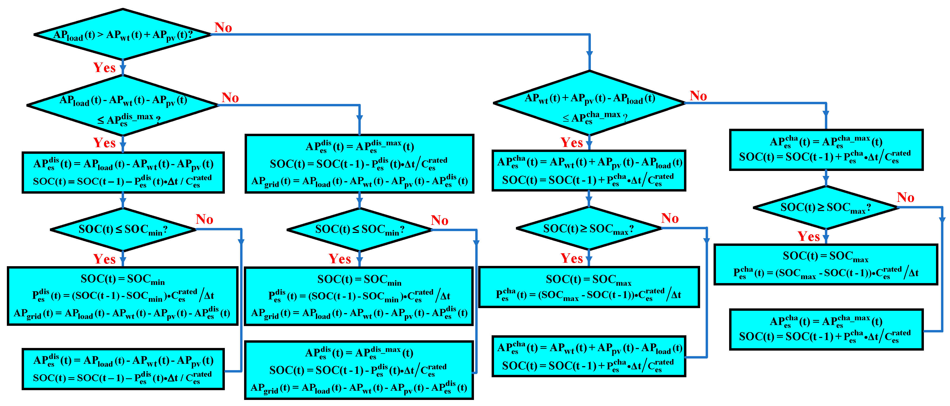
4.2. Power Output Strategy

The PV system and WTs priorly provide power for loads. However, the fluctuation of the PV system and WTs will probably lead to a surplus or shortage of power in the system. When the system’s power cannot meet the load requirements, the BESS will supply power until decreasing to the minimum SOC constraint. If the power is still insufficient, the system will purchase additional power. Conversely, during periods of sufficient power, the BESS will be charged to the maximum SOC constraints. If the BESS is fully charged, power from the WTs and solar panels will be abandoned. The specific output strategy is shown in Figure 4 below:

4.3. Optimization Algorithm

Optimizing the capacity for WTs, solar panels, and batteries is a problem with multiple variables and constraints. Conventional algorithms used to solve optimization problems include genetic algorithms, grey wolf algorithms, and particle swarm optimization (PSO). PSO simulates the optimization behavior of groups such as birds or fish. It performs well in solving multi-variable and multi-constraint optimization problems such as capacity configuration. The PSO optimization steps are capable of solving the optimization process of the problem solved in this paper. A set of results for the WTs, PV system, and BESS configuration can be seen as position parameters of a particle. The position constraints of the particle swarm represent the quantitative constraints of multiple sets of WT, PV, and BESS configuration results. By calculating the particle swarm fitness function, the total economic cost of multiple configuration results can be obtained. By continuously updating the velocity and position of the particle swarm, the optimal cost and corresponding WTs, solar panels, and battery configuration results can be obtained. The following steps outline the process: (1) Initialize particle swarm parameters, such as the initial velocity, population size, iteration times, speed range, and position of the particles. Calculate the fitness value of each particle based on its position and velocity. The fitness value is an objective function. (2) Update the individual best position, global best position, and global optimal fitness value. (3) Update the velocity and position of the particles based on the formal individual optimal position and global optimal position. (4) Repeat the above steps until the maximum iteration times are reached and output the result. The solving steps can be observed in Figure 5.

5. Example Analysis

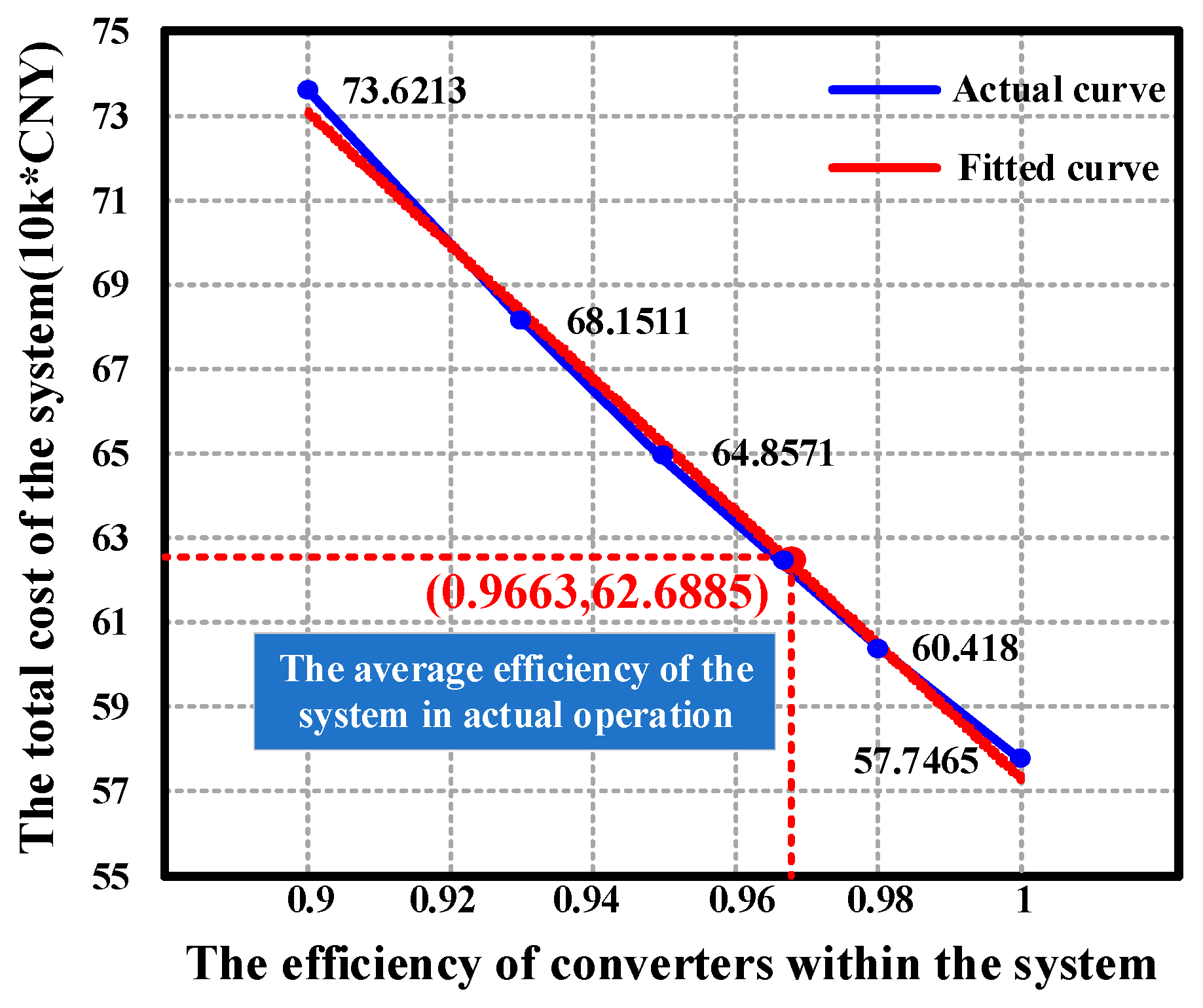
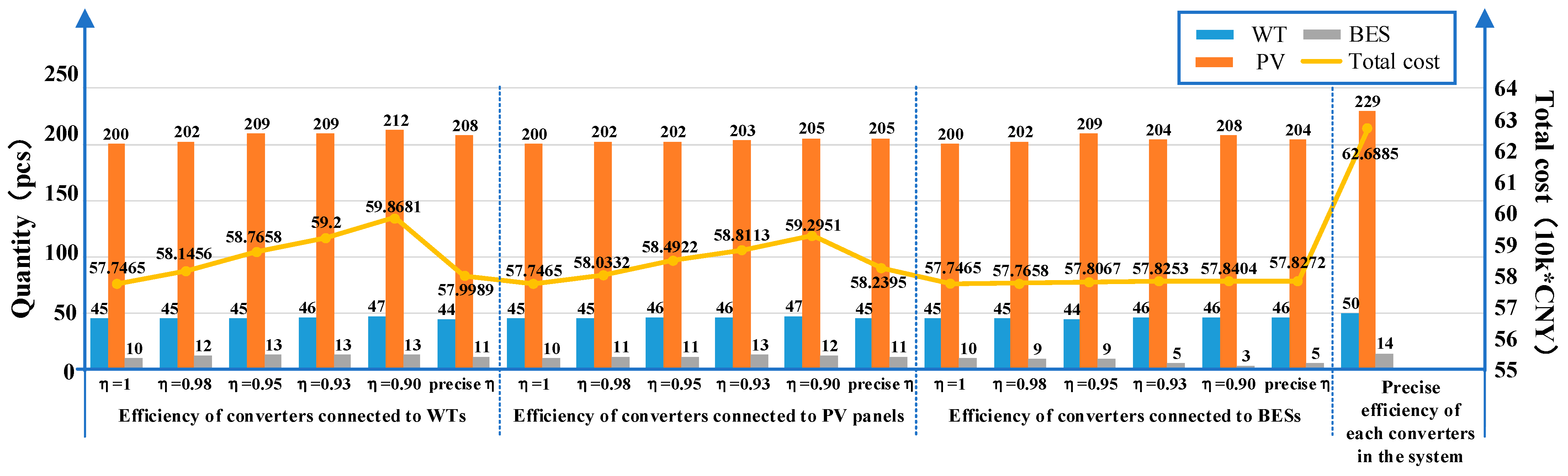
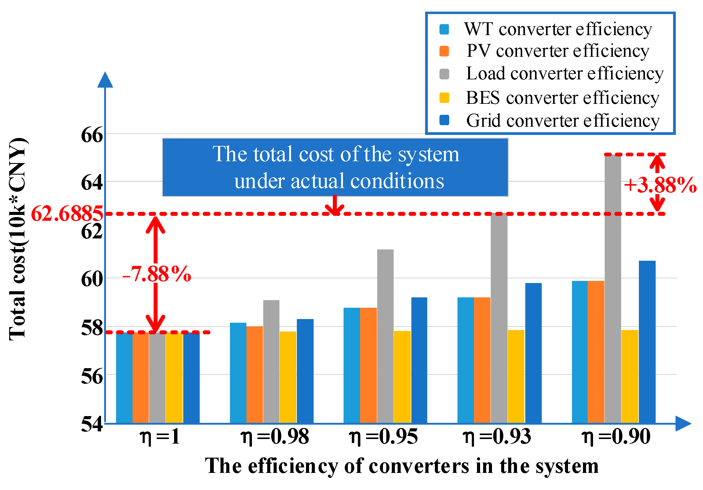
5.1. Example 1: DC Power System

This example is a small DC power system consisting of a DC 400 V bus and a WT–PV–BES–grid system, as depicted in Figure 6.

The type of power supply equipment and the quantity of the load will jointly affect the equipment parameter settings. The equipment parameter will then affect the selection of relevant converters. By analyzing the losses of commonly used converters and referring to the efficiency curve in the product manual, the types of converters in this example are reasonably selected. Specifically, the WT refers to the products manufactured by Bergey Windpower Co. (Norman, OK, USA). The PV module refers to the products made by SunPower Corporation (San Jose, CA, USA). The BESS refers to the products from LG Energy Solution (Seoul, Republic of Korea). The WT converter refers to the products manufactured Hefei Weimin Power Supply Co., Ltd. (Hefei, China), while the PV converter and the BES converter refer to the Sunny Boy and Sunny Boy Storage series products, respectively, manufactured by SMA Solar Technology AG (Niestetal, Germany).

Table 1. The DC power system parameters.

Component	Parameter	Value	Parameter	Value
WT [41,43]	The rated power (kW/pcs)	10	Cut-in wind speed (m/s)	3
	The rated wind speed (m/s)	11	Cut-out wind speed (m/s)	25
	Unit purchase price	3.86	Unit installation price	0.15
	Unit maintenance price	0.1	Lifespan (years)	20
PV [39,43]	The rated power (kW/pcs)	2	Unit purchase price	0.8
	Standard solar radiation intensity (kW/m2)	1	Unit installation price	0.03
	Coefficient of environmental temperature	4.7 × 10−3	Unit maintenance price	0.002
	Standard environmental temperature (°C)	25	Lifespan (years)	20
BES [44]	Battery charging efficiency	0.85	Unit purchase price	0.16
	Battery discharging efficiency	0.85	Unit installation price	0.005
	Maximum SOC	0.9	Unit maintenance price	0.002
	Minimum SOC	0.2	Lifespan (years)	1.36
	The rated capacity	6
Grid	Low purchase unit price	5.5 × 10−5	Medium purchase unit price	6.0 × 10−5
	High purchase unit price	8.5 × 10−5
Other	Discount rate (%)	4.75	The standard power waste penalty fee (10k*CNY)	1
	Time interval (h)	1	The standard penalty coefficient	0.2

and

Table 2. Parameters of the converter in the DC Power System.

Component	Parameter	Value	Parameter	Value
Coefficient of the efficiency curve	$a_{\mathrm{wt}}$ for WT converters	6.12 × 10−2	$a_{\mathrm{grid}}$ for grid converters	−2.28 × 10−4
	$b_{\mathrm{wt}}$ for WT converters	−5.50 × 10−1	$b_{\mathrm{grid}}$ for grid converters	−9.426
	$c_{\mathrm{wt}}$ for WT converters	98.64	$c_{\mathrm{grid}}$ for grid converters	98.02
	$a_{\mathrm{pv}}$ for PV converters	−2.588	$a_{\mathrm{ac}}$ for AC load converters	−7.39 × 10−1
	$b_{\mathrm{pv}}$ for PV converters	−9.02×10−1	$b_{\mathrm{ac}}$ for AC load converters	−10.71
	$c_{\mathrm{pv}}$ for PV converters	100.4	$c_{\mathrm{ac}}$ for AC load converters	99.52
	$a_{\mathrm{es}}$ for BESS converters	−2.56×10−1	$a_{\mathrm{dc}}$ for DC load converters	−2.14 × 10−1
	$b_{\mathrm{es}}$ for BESS converters	−7.025	$b_{\mathrm{dc}}$ for DC load converters	−4.86 × 10−1
	$c_{\mathrm{es}}$ for BESS converters	99.82	$c_{\mathrm{dc}}$ for DC load converters	98.97
Unit price	Purchase of WT converter	0.2	Installing of grid converter	0.02
	Installing of WT converter	0.03	Purchase of AC load converter	0.07
	Purchase of PV converter	0.02	Purchase of DC load converter	0.04
	Installing of PV converter	0.01	Installing of AC load converter	0.01
	Purchase of BES converter	0.05	Installing of DC load converter	0.01
	Installing of BES converter	0.01	Maintenance of converter	0.001
	Purchase of grid converter	0.1
Rated power	Grid converter (kW)	10	DC load converter (kW)	2
	AC load converter (kW)	5
Lifespan	Various types of converters (years)	10

display the specific values for the power system and converter parameters, respectively. The data in Table 2 are derived from the testing of our prototype. The unit of price for the WT, PV system, BES, and converters is expressed as CNY 10,000 per unit (10k*CNY/pcs), and the unit of price for the grid is expressed as CNY 10,000 per kWh (10k*CNY/kWh).

This paper selects several fixed efficiency values for the converters in the system. The system costs and the configuration quantities of WTs, solar panels, and BESS are calculated. Compared to using an accurate efficiency model for converters, it can be seen that the results of the various costs and the quantity of WTs, PV panels, and BESS have changed, as shown in

Table 3. The quantity configurations of equipment and the corresponding system expenses under different converter efficiencies.

The Efficiency of Each Converter in the System	${\mathit{N}}_{\mathbf{p}.1}$	${\mathit{N}}_{\mathbf{p}.2}$	${\mathit{N}}_{\mathbf{p}.3}$	${\mathit{C}}_{\mathbf{ep}}$	${\mathit{C}}_{\mathbf{ei}}$	${\mathit{C}}_{\mathbf{peg}}$	${\mathit{C}}_{\mathbf{ewp}}$	${\mathit{C}}_{\mathbf{em}}$	${\mathit{C}}_{\mathbf{t}}$
1	45	200	10	31.2712	1.8819	19.1365	0.3269	5.1300	57.7465
0.98	46	223	14	33.6512	2.0067	19.1516	0.3245	5.2840	60.4180
0.95	50	244	22	37.4272	2.1953	19.1513	0.3413	5.7420	64.8571
0.93	53	265	25	40.2083	2.3398	19.1490	0.3640	6.0900	68.1511
0.90	59	280	37	44.7811	2.5603	19.1496	0.3863	6.7440	73.6213
Precise efficiency model proposed in this paper	50	229	14	35.3677	2.0928	19.1406	0.3914	5.6960	62.6885

. The unit for different costs is CNY 10,000 (10k*CNY). Specifically, with every 1% decrease in the total system efficiency, the quantity of WTs, PV panels, and BESSs will increase by approximately 1.4, 8, and 2.7 units, respectively. The system’s total cost will rise by approximately CNY 15,875. Moreover, the extent of changes in quantity and cost is influenced by system parameters, such as the lifespan, capacity, and cost of the power supply equipment.

In addition, the efficiency–total cost curve is fitted, as shown in Figure 7. By observing the fitted curves, the average costs of the system under the precise converter efficiency model can be accurately estimated. The conclusion indicates that the system’s total efficiency is approximately 96.63%. Compared to the total efficiency of 100%, costs increased by CNY 49,420, approximately 8.56%.

When only one type of converter efficiency changes, the other converters’ efficiencies are considered to be 100%. The obtained configuration results and various costs definitely will be inaccurate, as shown in Figure 8. Compared with the precise efficiency model presented above, when only the efficiency variation of the WT converter is considered, the maximum variations in the quantities of WTs, PV panels, and BESSs are −12%, −12.66%, and −28.57%, respectively. Similarly, when only the efficiency variation of the PV converter is considered, the maximum quantity changes of WTs, PV panels, and BESSs are −10%, −12.66%, and −28.57%, respectively. When only the efficiency variation of the BESS converter is considered, the maximum quantity changes are −10%, −12.66%, and −78.57%, respectively. When the efficiency of the three types of converters changes individually, the maximum change in total cost is −7.88% for each.

Different converters have varying effects on the overall cost. Among them, changing the converter’s efficiency connected to loads has the greatest impact on total cost. The total cost gradually decreases when the efficiency of grid converters, PV converters, and WT converters change independently. When the efficiency of one type of converter changes, the efficiencies of the other converters remain at 100%. The efficiency change of the converter connected to the BESS has minimal impact on the total cost. Overall, as shown in Figure 9, the system’s minimum cost is 7.88% lower than the actual cost.

The above analysis shows the importance of a precise converter efficiency model. However, this model is rarely considered in most studies. We compared the converter efficiency model used in different literature [4,6,12,13] with the one introduced in this paper; the variations in system configuration results and costs are illustrated in Figure 10.

5.2. Example 2: AC Power System

This example is an AC power system consisting of an AC 220 V bus and a WT–PV–BES–grid system, as depicted in Figure 11.

Table 4. The AC power system parameters.

Component	Parameter	Value	Parameter	Value
WT [41,43]	The rated power (kW/pcs)	5	Cut-in wind speed (m/s)	3
	The rated wind speed (m/s)	11	Cut-out wind speed (m/s)	25
	Unit purchase price	3.86	Unit installation price	0.15
	Unit maintenance price	0.1	Lifespan (years)	20
PV [39,43]	The rated power (kW/pcs)	1	Unit purchase price	0.8
	Standard solar radiation intensity (kW/m2)	1	Unit installation price	0.03
	Coefficient of environmental temperature	4.7 × 10−3	Unit maintenance price	0.002
	Standard environmental temperature (°C)	25	Lifespan (years)	20
BES [44]	Battery charging efficiency	0.85	Unit purchase price	0.16
	Battery discharging efficiency	0.85	Unit installation price	0.005
	Maximum SOC	0.9	Unit maintenance price	0.002
	Minimum SOC	0.2	Lifespan (years)	1.36
	The rated capacity	2
Grid	Low purchase unit price	5.5 × 10−5	Medium purchase unit price	6.0 × 10−5
	High purchase unit price	8.5 × 10−5
Other	Discount rate (%)	4.75	The standard power waste penalty fee (10k*CNY)	1
	Time interval (h)	1	The standard penalty coefficient	0.2

and

Table 5. Parameters of the converter in the AC Power System.

Component	Parameter	Value	Parameter	Value
Coefficient of the efficiency curve	$a_{\mathrm{pv}}$ for PV converters	−5.16	$c_{\mathrm{es}}$ for BESS converters	97.8
	$b_{\mathrm{pv}}$ for PV converters	−4.56 × 10−1	$a_{\mathrm{dc}}$ for DC load converters	−2.14 × 10−1
	$c_{\mathrm{pv}}$ for PV converters	100.5	$b_{\mathrm{dc}}$ for DC load converters	−4.86 × 10−1
	$a_{\mathrm{es}}$ for BESS converters	3.11 × 10−1	$c_{\mathrm{dc}}$ for DC load converters	98.97
	$b_{\mathrm{es}}$ for BESS converters	−2.406

, respectively, present the specific values of the system parameters and converter parameters for Example 2. The purchase unit price, rated power, and lifespan parameters of the converter are the same as those in Example 1.

Adopting the same comparison method as in Example 1, the power supply equipment’s quantity configuration results and the system’s corresponding costs under different converter efficiency models are shown in

Table 6. The quantity configurations of equipment and the corresponding system expenses under different converter efficiencies.

The Efficiency of Each Converter in the System	${\mathit{N}}_{\mathbf{p}.1}$	${\mathit{N}}_{\mathbf{p}.2}$	${\mathit{N}}_{\mathbf{p}.3}$	${\mathit{C}}_{\mathbf{ep}}$	${\mathit{C}}_{\mathbf{ei}}$	${\mathit{C}}_{\mathbf{peg}}$	${\mathit{C}}_{\mathbf{ewp}}$	${\mathit{C}}_{\mathbf{em}}$	${\mathit{C}}_{\mathbf{t}}$
1	22	96	6	13.8863	0.6776	4.9229	0.2957	2.5949	22.3774
0.98	23	95	6	14.1241	0.6858	4.9211	0.3221	2.6930	22.7461
0.95	23	103	6	14.6473	0.7149	4.9237	0.3273	2.7171	23.3303
0.93	24	101	7	14.9503	0.7245	4.9218	0.3486	2.8153	23.7605
0.90	24	112	6	15.5391	0.7594	4.9244	0.3606	2.8454	24.4289
Precise efficiency model proposed in this paper	23	98	5	14.1896	0.6915	4.9215	0.3275	2.6990	22.8291

.

When the total efficiency decreases by 1%, the system’s total cost will increase by approximately CNY 2052. Moreover, when the system’s total efficiency continues to decrease, the first step is to increase PV panel quantity and reduce BES utilization to supply power to minimize the total cost. When the total cost of the above method exceeds the total cost obtained by increasing the number of BESSs and decreasing the PV panel quantity, the method should be changed to reduce the PV panel quantity and simultaneously increase the BESS quantity. When the total cost of the above two methods is greater than the total cost obtained by increasing the number of WTs, then the method should be changed to improve WT quantity while reducing BES and PV panel quantity.

By observing the fitted curves, the average cost of the system under the precise converter efficiency model can be accurately estimated. The conclusion indicates that the system’s total efficiency is approximately 97.64%. Compared to the total efficiency of 100%, costs increased by CNY 4517, approximately 2.02%, as shown in Figure 12.

The quantity of power supply equipment and the total cost in the system vary greatly with different converter efficiencies, as shown in Figure 13. When the efficiency of one type of converter varies individually, the other converters’ efficiencies are considered to be 100%. Compared with the precise efficiency model presented above, the maximum variations in the quantities of WTs, PV panels, and BESSs are ±4.35%, −4.08%, and +20%, respectively, when the efficiency variation is only in the converter used in the PV systems. Similarly, when the efficiency of converters connected to the BESS varies individually, the maximum quantity changes of WTs, PV panels, and BESSs are −4.35%, −4.08%, and −40%, respectively. When the efficiency of the two types of converters changes individually, the maximum change in total costs is −1.98% for each.

The impact of each type of converter efficiency on total cost is different. The extent of cost changes gradually decreases after changing the efficiency of the load converters, PV converters, and BES converters. The maximum change in total cost is +3.13%, as shown in Figure 14.

We compared the converter efficiencies used in different literature [11,16,44] with the model presented above; the variations in system configuration results and costs are illustrated in Figure 15.

From the above two examples, some conclusions can be drawn. In different power systems, due to factors such as system-rated power and power source capacity, the configuration quantity of the power supply equipment is completely different. The extent of variation in the equipment quantity also differs during the process of converter efficiency changes. In the same power system, due to factors such as the cost and lifespan of the power sources, and the cost and efficiency of the converters, the degree of variation in quantity and total cost is relatively small. In addition, when the system efficiency changes, the priority of adjusting the quantity of different power sources will be determined by the relevant parameters of both the power sources and the converters.

The overall system expenditure is influenced by both the quantity of power supply equipment and the efficiency of the converters. Furthermore, the total cost is negatively linearly related to the system’s overall efficiency. This conclusion can provide a reference for predicting the comprehensive efficiency of complex power systems with multiple generation sources and converters. In particular, the overall efficiency is mainly affected by the large-capacity power supplies and converters connected with them. The overall efficiency in different systems is generally more than 95%.

6. Conclusions

This paper establishes an advanced mathematical framework with corresponding boundary constraints for WT–PV–BES–grid–load, incorporating precise converter efficiency models. The optimization results of WT–PV–BES configuration and the total cost of the EPS are compared under three conditions: ignoring the efficiency model of the PEC, using the fixed efficiency model of the PEC, and using the proposed accurate efficiency model of the PEC. The results indicate that neglecting PEC efficiency characterization significantly affects the accuracy and effectiveness of WT–PV–BES system configurations. Apparently, the proposed accurate efficiency PEC model can be expected to provide reference and guidance for future research on EPS configuration optimization.

References

1. Anoune, K.; Bouya, M.; Astito, A.; Abdellah, A.B. Sizing methods and optimization techniques for PV-wind based hybrid renewable energy system: A review. Renew. Sustain. Energy Rev. 2018, 93, 652–673. [Google Scholar] [CrossRef]
2. Han, Z.; Li, Z.; Wang, W.; Liu, W.; Ma, Q.; Sun, S.; Liu, H.; Zhang, Q.; Cao, Y. Multi-Time Optimization Scheduling Strategy for Integrated Energy Systems Considering Multiple Controllable Loads and Carbon Capture Plants. Energies 2024, 17, 5995. [Google Scholar] [CrossRef]
3. Zhang, J.; Li, J. Revolution in renewables: Integration of green hydrogen for a sustainable future. Energies 2024, 17, 4148. [Google Scholar] [CrossRef]
4. Zhang, Y.; Hua, Q.S.; Sun, L.; Liu, Q. Life cycle optimization of renewable energy systems configuration with hybrid battery/hydrogen storage: A comparative study. J. Energy Storage 2020, 30, 101470. [Google Scholar] [CrossRef]
5. Yang, J.; Yang, Z.; Duan, Y. Optimal capacity and operation strategy of a solar-wind hybrid renewable energy system. Energy Convers. Manag. 2021, 244, 114519. [Google Scholar] [CrossRef]
6. Xiao, Y.; Zou, C.; Dong, M.; Chi, H.; Yan, Y.; Jiang, S. Feasibility study: Economic and technical analysis of optimal configuration and operation of a hybrid CSP/PV/wind power cogeneration system with energy storage. Renew. Energy 2024, 225, 120273. [Google Scholar] [CrossRef]
7. Emad, D.; El-Hameed, M.A.; El-Fergany, A.A. Optimal techno-economic design of hybrid PV/wind system comprising battery energy storage: Case study for a remote area. Energy Convers. Manag. 2021, 249, 114847. [Google Scholar] [CrossRef]
8. Megaptche, C.A.M.; Musau, P.M.; Tjahè, A.V.; Kim, H.; Waita, S.; Aduda, B.O. Demand response-fuzzy inference system controller in the multi-objective optimization design of a photovoltaic/wind turbine/battery/supercapacitor and diesel system: Case of healthcare facility. Energy Convers. Manag. 2023, 291, 117245. [Google Scholar] [CrossRef]
9. Javed, M.S.; Song, A.; Ma, T. Techno-economic assessment of a stand-alone hybrid solar-wind-battery system for a remote island using genetic algorithm. Energy 2019, 176, 704–717. [Google Scholar] [CrossRef]
10. Arabi-Nowdeh, S.; Nasri, S.; Saftjani, P.B.; Naderipour, A.; Abdul-Malek, Z.; Kamyab, H.; Jafar-Nowdeh, A. Multi-criteria optimal design of hybrid clean energy system with battery storage considering off-and on-grid application. J. Clean. Prod. 2021, 290, 125808. [Google Scholar] [CrossRef]
11. Naderipour, A.; Ramtin, A.R.; Abdullah, A.; Marzbali, M.H.; Nowdeh, S.A.; Kamyab, H. Hybrid energy system optimization with battery storage for remote area application considering loss of energy probability and economic analysis. Energy 2022, 239, 122303. [Google Scholar] [CrossRef]
12. Tebibel, H. Methodology for multi-objective optimization of wind turbine/battery/electrolyzer system for decentralized clean hydrogen production using an adapted power management strategy for low wind speed conditions. Energy Convers. Manag. 2021, 238, 114125. [Google Scholar] [CrossRef]
13. Nyeche, E.N.; Diemuodeke, E.O. Modelling and optimisation of a hybrid PV-wind turbine-pumped hydro storage energy system for mini-grid application in coastline communities. J. Clean. Prod. 2020, 250, 119578. [Google Scholar] [CrossRef]
14. Al-Ghussain, L.; Samu, R.; Taylan, O.; Fahrioglu, M. Sizing renewable energy systems with energy storage systems in microgrids for maximum cost-efficient utilization of renewable energy resources. Sustain. Cities Soc. 2020, 55, 102059. [Google Scholar] [CrossRef]
15. Medghalchi, Z.; Taylan, O. A novel hybrid optimization framework for sizing renewable energy systems integrated with energy storage systems with solar photovoltaics, wind, battery and electrolyzer-fuel cell. Energy Convers. Manag. 2023, 294, 117594. [Google Scholar] [CrossRef]
16. Xu, X.; Hu, W.; Cao, D.; Huang, Q.; Chen, C.; Chen, Z. Optimized sizing of a standalone PV-wind-hydropower station with pumped-storage installation hybrid energy system. Renew. Energy 2020, 147, 1418–1431. [Google Scholar] [CrossRef]
17. Jamshidi, M.; Askarzadeh, A. Techno-economic analysis and size optimization of an off-grid hybrid photovoltaic, fuel cell and diesel generator system. Sustain. Cities Soc. 2019, 44, 310–320. [Google Scholar] [CrossRef]
18. Hou, H.; Xu, T.; Wu, X.; Wang, H.; Tang, A.; Chen, Y. Optimal capacity configuration of the wind-photovoltaic-storage hybrid power system based on gravity energy storage system. Appl. Energy 2020, 271, 115052. [Google Scholar] [CrossRef]
19. Emrani, A.; Berrada, A.; Arechkik, A.; Bakhouya, M. Improved techno-economic optimization of an off-grid hybrid solar/wind/gravity energy storage system based on performance indicators. J. Energy Storage 2022, 49, 104163. [Google Scholar] [CrossRef]
20. Iqbal, R.; Liu, Y.; Zeng, Y.; Zhang, Q.; Zeeshan, M. Comparative study based on techno-economics analysis of different shipboard microgrid systems comprising PV/wind/fuel cell/battery/diesel generator with two battery technologies: A step toward green maritime transportation. Renew. Energy 2024, 221, 119670. [Google Scholar] [CrossRef]
21. Ren, Y.; Jin, K.; Gong, C.; Hu, J.; Liu, D.; Jing, X.; Zhang, K. Modelling and capacity allocation optimization of a combined pumped storage/wind/photovoltaic/hydrogen production system based on the consumption of surplus wind and photovoltaics and reduction of hydrogen production cost. Energy Convers. Manag. 2023, 296, 117662. [Google Scholar] [CrossRef]
22. Alshammari, N.; Asumadu, J. Optimum unit sizing of hybrid renewable energy system utilizing harmony search, Jaya and particle swarm optimization algorithms. Sustain. Cities Soc. 2020, 60, 102255. [Google Scholar] [CrossRef]
23. Arasteh, A.; Alemi, P.; Beiraghi, M. Optimal allocation of photovoltaic/wind energy system in distribution network using meta-heuristic algorithm. Appl. Soft Comput. 2021, 109, 107594. [Google Scholar] [CrossRef]
24. Abdel-Mawgoud, H.; Ali, A.; Kamel, S.; Rahmann, C.; Abdel-Moamen, M.A. A modified manta ray foraging optimizer for planning inverter-based photovoltaic with battery energy storage system and wind turbine in distribution networks. IEEE Access 2021, 9, 91062–91079. [Google Scholar] [CrossRef]
25. Alzahrani, A.; Hayat, M.A.; Khan, A.; Hafeez, G.; Khan, F.A.; Khan, M.I.; Ali, S. Optimum sizing of stand-alone microgrids: Wind turbine, solar photovoltaic, and energy storage system. J. Energy Storage 2023, 73, 108611. [Google Scholar] [CrossRef]
26. Chen, X.; Dong, W.; Yang, Q. Robust optimal capacity planning of grid-connected microgrid considering energy management under multi-dimensional uncertainties. Appl. Energy 2022, 323, 119642. [Google Scholar] [CrossRef]
27. Sahoo, B.; Routray, S.K.; Rout, P.K. AC, DC, and hybrid control strategies for smart microgrid application: A review. Int. Trans. Electr. Energy Syst. 2021, 31, e12683. [Google Scholar] [CrossRef]
28. Zhu, B.; Wang, H.; Vilathgamuwa, D.M. Single-switch high step-up boost converter based on a novel voltage multiplier. IET Power Electron. 2019, 12, 3732–3738. [Google Scholar] [CrossRef]
29. Zhu, B.; Yang, Y.; Wang, K.; Liu, J.; Vilathgamuwa, D.M. High transformer utilization ratio and high voltage conversion gain flyback converter for photovoltaic application. IEEE Trans. Ind. Appl. 2024, 60, 2840–2851. [Google Scholar] [CrossRef]
30. Shahin, A.; Payman, A.; Martin, J.P.; Pierfederici, S.; Meibody-Tabar, F. Approximate novel loss formulae estimation for optimization of power controller of DC/DC converter. In Proceedings of the IECON 2010-36th Annual Conference on IEEE Industrial Electronics Society, Glendale, AZ, USA, 7–10 November 2010; IEEE: New York, NY, USA, 2010; pp. 373–378. [Google Scholar]
31. Zhu, B.; Liu, Y.; Zhi, S.; Wang, K.; Liu, J. A family of bipolar high step-up zeta–buck–boost converter based on “coat circuit”. IEEE Trans. Power Electron. 2023, 38, 3328–3339. [Google Scholar] [CrossRef]
32. Zhu, B.; Wang, H.; Zhang, Y.; Chen, S. Buck-based active-clamp circuit for current-fed isolated DC–DC converters. IEEE Trans. Power Electron. 2022, 37, 4337–4345. [Google Scholar] [CrossRef]
33. Kasprzyk, L.; Tomczewski, A.; Pietracho, R.; Mielcarek, A.; Nadolny, Z.; Tomczewski, K.; Trzmiel, G.; Alemany, J. Optimization of a PV-Wind hybrid power supply structure with electrochemical storage intended for supplying a load with known characteristics. Energies 2020, 13, 6143. [Google Scholar] [CrossRef]
34. Geng, C.; Shi, Z.; Chen, X.; Sun, Z.; Jin, Y.; Shi, T.; Wu, X. Stochastic Capacity Optimization of an Integrated BFGCC–MSHS–Wind–Solar Energy System for the Decarbonization of a Steelmaking Plant. Energies 2024, 17, 2994. [Google Scholar] [CrossRef]
35. Al Shereiqi, A.; Al-Hinai, A.; Albadi, M.; Al-Abri, R. Optimal sizing of a hybrid wind-photovoltaic-battery plant to mitigate output fluctuations in a grid-connected system. Energies 2020, 13, 3015. [Google Scholar] [CrossRef]
36. Zhong, X.; Sun, X.; Wu, Y. A capacity optimization method for a hybrid energy storage microgrid system based on an augmented ε-constraint method. Energies 2022, 15, 7593. [Google Scholar] [CrossRef]
37. Weng, Z.; Zhou, J.; Zhan, Z. Reliability evaluation of standalone microgrid based on sequential Monte Carlo simulation method. Energies 2022, 15, 6706. [Google Scholar] [CrossRef]
38. Dong, J.; Dou, Z.; Si, S.; Wang, Z.; Liu, L. Optimization of capacity configuration of wind–solar–diesel–storage using improved sparrow search algorithm. J. Electr. Eng. Technol. 2022, 17, 1–14. [Google Scholar] [CrossRef]
39. He, Y.; Guo, S.; Zhou, J.; Wu, F.; Huang, J.; Pei, H. The quantitative techno-economic comparisons and multi-objective capacity optimization of wind-photovoltaic hybrid power system considering different energy storage technologies. Energy Convers. Manag. 2021, 229, 113779. [Google Scholar] [CrossRef]
40. Wang, J.; Deng, H.; Qi, X. Cost-based site and capacity optimization of multi-energy storage system in the regional integrated energy networks. Energy 2022, 261, 125240. [Google Scholar] [CrossRef]
41. Yang, J.; Yang, Z.; Duan, Y. Capacity optimization and feasibility assessment of solar-wind hybrid renewable energy systems in China. J. Clean. Prod. 2022, 368, 133139. [Google Scholar] [CrossRef]
42. Yi, T.; Ye, H.; Li, Q.; Zhang, C.; Ren, W.; Tao, Z. Energy storage capacity optimization of wind-energy storage hybrid power plant based on dynamic control strategy. J. Energy Storage 2022, 55, 105372. [Google Scholar] [CrossRef]
43. Taha, H.A.; Alham, M.H.; Youssef, H.K.M. Multi-objective optimization for optimal allocation and coordination of wind and solar DGs, BESSs and capacitors in presence of demand response. IEEE Access 2022, 10, 16225–16241. [Google Scholar] [CrossRef]
44. Chennaif, M.; Zahboune, H.; Elhafyani, M.; Zouggar, S. Electric System Cascade Extended Analysis for optimal sizing of an autonomous hybrid CSP/PV/wind system with Battery Energy Storage System and thermal energy storage. Energy 2021, 227, 120444. [Google Scholar] [CrossRef]
Figure 1. Typical converter efficiency curve.
Energies 18 01320 g001
Figure 2. Power supply system structure description: (a) typical DC power system structure; (b) typical AC power system structure.
Energies 18 01320 g002
Figure 3. Loss proportion of different devices.
Energies 18 01320 g003
Figure 4. Power output process.
Energies 18 01320 g004
Figure 5. Optimization process of the power system based on PSO.
Energies 18 01320 g005
Figure 6. The structure of the DC power system.
Energies 18 01320 g006
Figure 7. The total cost under different system efficiencies.
Energies 18 01320 g007
Figure 8. Power supply equipment configuration results and total costs under different efficiencies of each type of converter.
Energies 18 01320 g008
Figure 9. The total cost under different efficiencies of each type of converter.
Energies 18 01320 g009
Figure 10. The comparison between the converter efficiency models in different literature and the precise efficiency model proposed in this paper [4,6,12,13].
Energies 18 01320 g010
Figure 11. The structure of AC power system.
Energies 18 01320 g011
Figure 12. The total cost under different system efficiencies.
Energies 18 01320 g012
Figure 13. Power supply configuration results and total cost under different efficiencies of each type of converter.
Energies 18 01320 g013
Figure 14. The total costs under different efficiencies of each type of converter.
Energies 18 01320 g014
Figure 15. The comparison between the converter efficiency models in different literature and the precise efficiency model proposed in this paper [11,16,44].
Energies 18 01320 g015