A Physical-Based Electro-Thermal Model for a Prismatic LFP Lithium-Ion Cell Thermal Analysis

Abstract

This article presents an electro-thermal model of a prismatic lithium-ion cell, integrating physics-based models for capacity and resistance estimation. A 100 Ah prismatic cell with LFP-based chemistry was selected for analysis. A comprehensive experimental campaign was conducted to determine electrical parameters and assess their dependencies on temperature and C-rate. Capacity tests were conducted to characterize the cell’s capacity, while an OCV test was used to evaluate its open circuit voltage. Additionally, Hybrid Pulse Power Characterization tests were performed to determine the cell’s internal resistive-capacitive parameters. To describe the temperature dependence of the cell’s capacity, a physics-based Galushkin model is proposed. An Arrhenius model is used to represent the temperature dependence of resistances. The integration of physics-based models significantly reduces the required test matrix for model calibration, as temperature-dependent behavior is effectively predicted. The electrical response is represented using a first-order equivalent circuit model, while thermal behavior is described through a nodal network thermal model. Model validation was conducted under real driving emissions cycles at various temperatures, achieving a root mean square error below 1% in all cases. Furthermore, a comparative study of different cell cooling strategies is presented to identify the most effective approach for temperature control during ultra-fast charging. The results show that side cooling achieves a 36% lower temperature at the end of the charging process compared to base cooling.

1. Introduction

Nowadays, more and more manufacturers are converting their vehicle fleets into electrified vehicles [1], which include battery electric vehicles or hybrid vehicles [2]. This conversion is because many national and international regulations are pushing in the direction of reducing greenhouse gas emissions and pollutants [3], and, in this context, electrified vehicles can certainly contribute significantly [4]. The battery technology most used in the automotive field is one based on lithium-ion chemistry [5], because, in addition to being characterized by larger values of energy density and power density than lead acid batteries [6], it is also characterized by the absence of a self-discharge effect and, compared with other competing chemicals, by longer lifespan [7]. Nevertheless, lithium-ion batteries have many limitations, especially from a thermal point of view: a lithium-ion battery only works well in a very narrow range of temperatures, between around 15 °C and 35 °C [8]. Problems can arise both at very high temperatures [9] and at very low temperatures: at very high temperatures, there may be a risk of thermal runaway [10], i.e., an uncontrolled temperature increase that can lead to catastrophic events such as fires and explosions [11]; similarly, at very low temperatures [12], dangerous phenomena such as the formation of dendrites inside the cells can occur, which can lead to short-circuit conditions and finally to very dangerous conditions [13]. Hence, electro-thermal models are urgently needed to accurately describe the behavior of the battery and that allow the prediction of what the thermal evolution of the battery will be during the critical phases of operation [14].

In the scientific literature, there are several works dealing with the electro-thermal modeling of lithium-ion batteries: the bibliographic review analyzed in this case is about 0D/1D models, which are the object of this work. Damay et al. [15] introduced a lumped thermal model for a prismatic cell. The heat flows from the central node only towards the wide lateral walls of the cell; other conductive resistances are provided between the various surface nodes of the battery. Damay et al. do not propose a combined electro-thermal model, differently from what it is proposed here, but they calculate only the resistive parameters useful for estimating heat generation. Firouz et al. [16] developed a combined electro-thermal model for a lithium-ion capacitor. They propose the use of a second order model for the electrical part which results in greater precision but has the disadvantage of a higher computational cost and calibration complexity, having to calibrate variables with a short time constant and a long time constant. For the thermal part, a nodal model is also proposed in this case. Pan et al. [17] showed in their work a pseudo-3D electro-thermal model. The electric part of the model consists of a second order equivalent circuit model. An experimental campaign was carried out to calibrate the resistive parameters of the cell, but the behavior of the cell in a wide range of charge/discharge rates was not analyzed: the parameters were calibrated only for two discharges rates. The thermal model consists of a nodal network composed by terminal nodes, surface nodes, and central nodes. Chen et al. [18] put forward an electro-thermal model composed of a second order equivalent circuit model and a nodal network representing the thermal model solved with the finite difference method: the model results in a better description than the nodal network, but it is also characterized by higher computational time and cost, which makes it unsuitable for online applications compared to a lumped thermal model. Akbarzadeh et al. [19] explored an analysis of a nodal electro-thermal model. A nominal value of the internal resistance of the cell was used to calculate the heat generation; therefore, the great variability of the internal resistive parameters with the state of charge and charge/discharge rate was not considered. An incorrect estimation of these parameters clearly led to an inaccurate estimation of the heat generation and input of the thermal model. Xiao et al. [20] introduced a nodal thermal model. The model consists of a series of layers, differentiated into surface layers and core layers, for the active part of the battery. In this case, however, there was no analysis of the electrical part or of the internal resistive parameters of the battery and the estimation of heat generation was based on an estimation of the open circuit voltage with a charge/discharge of the cell at a very low current.

Recent studies, such as those by Zhou et al. [21] and Wang et al. [22], highlight the importance of advanced electro-thermal modeling to improve heat transfer predictions and electrochemical–thermal coupling in Li-ion batteries. These works reinforce the need for physically motivated models that balance computational efficiency and predictive accuracy.

In this work, an electro-thermal model of a 0D/1D prismatic cell is proposed. The main novelty consists in the fact that the lumped electro-thermal model, experimentally calibrated, is coupled with physical extrapolation models which allow the reduction of the test matrix needed for the calibration. To the best of the authors’ knowledge, this prismatic cell model, coupled with two physical models, represents a novelty in the literature. Due to this coupling, the proposed model shows both the advantages of lumped electro-thermal modelling (less computational time than an electrochemical model and no need of knowledge of diffusion and electrochemical phenomena) and the advantages of physical extrapolation models which allow the reduction of the test matrix needed for model calibration. In fact, one of the main drawbacks of a lumped model is that it needs lots of testing to calibrate parameters in different operation scenarios; in this way, the test matrix area is greatly reduced.

The proposed model was validated in highly dynamic conditions and then it was used for analyzing cooling strategy options for a prismatic cell. Although this model is coupled with physical extrapolation models (Arrhenius model for the resistive parameter behaviors and Galushkin model for the cell capacity behavior), it does not require any knowledge of the phenomena that occur inside the cell, such as diffusion, mass transport, and electrochemical phenomena, and therefore is much easier to calibrate and requires much shorter calculation times than a physical model. To evaluate the goodness of the lumped model coupled with the physical models, the validation process was repeated at different temperatures to understand the goodness of the prediction at very high ambient temperatures (35 °C), mild ambient temperatures (10 °C), and cold ambient temperature (0 °C).

The electrical model is based on a first order equivalent circuit model whose parameters were calibrated with a large experimental campaign; the electric parameters were calibrated considering five discharge/charge rates, ten state of charge stages, and three temperatures, giving a perfect knowledge of the variation of the electrical parameters of the cell throughout several operational conditions (maps of each electrical parameters are provided); the thermal part was modeled with a validated lumped thermal model composed by nine nodes. Thus, the model constructed was validated in very dynamic operating conditions.

One of the key advantages of the electro-thermal model presented in this work is its versatility for both off-line and online applications. It can be effectively used for battery pack cooling studies, as demonstrated in this work, while also being integrated into real-time battery management system (BMS) control strategies.

Moreover, its coupling with physics-based extrapolation models significantly reduces the required test matrix, minimizes model calibration time, and shortens testing efforts, making it highly efficient for practical implementation.

The final section of this work presents a simulated analysis of various cooling strategies for a prismatic cell. Given that many manufacturers prefer prismatic cells for battery pack construction, the ability to use 0D/1D models for thermal management simulation holds significant value. This is not only beneficial for academic research but also for industrial applications, as it enables the prototyping of battery cooling systems based on the optimal cooling strategy identified through simulations.

Thus, the proposed prismatic cell model combines the advantages of both physics-based models—which provide a detailed understanding of parameter variations with state of charge (SOC), current, and temperature—and lumped models, which offer low computational cost, fewer calibration parameters, and reduced model complexity. This balance ensures high accuracy while maintaining computational efficiency, making it a valuable tool for both research and industry.

The work proposed here is made up of seven sections: Section 1 is the introduction; Section 2 concerns the experimental apparatus designed and built for the realization of the experimental campaign and the characteristics of the cell considered for this analysis; Section 3 concerns the theoretical description of the proposed electro-thermal model, consisting of a first subsection concerning the equivalent circuit model, a second subsection concerning the heat generation model, and a third subsection concerning the thermal model; Section 4 deals with the experimental characterization of electrical parameters through a capacity test to map the cell capacity, an Open Circuit Voltage test (OCV test) to map the OCV, and a Hybrid Power Pulse Characterization test (HPPC test) to map the resistive and capacitive parameters of the cell; the calibration procedure of the thermal parameters is also shown; Section 5 deals with model validation with a real driving emission (RDE) cycle; Section 6 concerns the study of the cooling strategies of a prismatic cell; finally, Section 7 concerns the conclusions of this work.

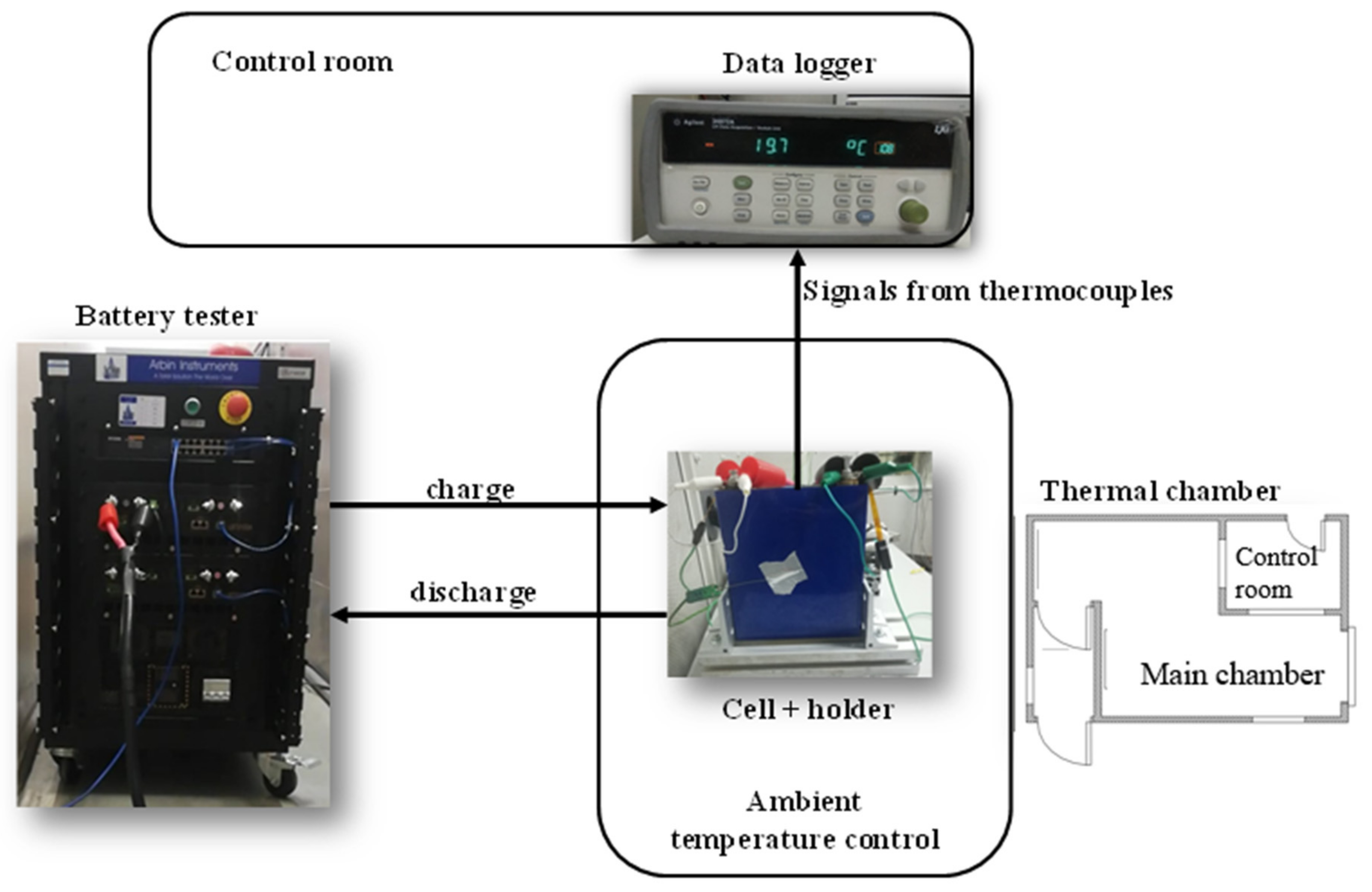
2. Experimental Tools & Selected Cell

The cell used for this work is an LFP prismatic cell. The cell’s main characteristics are summarized in

Table 1. Prismatic cell characteristics from datasheet.

Format	Prismatic
Length [mm]	207.6 ± 1.0
Width [mm]	173.9 ± 1.0
Height [mm]	28.8 ± 1.0
Weight [kg]	2.1 ± 0.05
Chemistry	LFP
Nominal voltage [V]	3.2
Nominal capacity [Ah]	100
Discharge cut-off voltage [V]	2.5
Charge cut-off voltage [V]	3.65
Discharge temperature range [°C]	[−30–55]
Charge temperature range [°C]	[0–45]
Storage temperature range [°C]	[−20–45]

.

Due to the charging and discharging rate limits of the cell, it was possible to discharge the cell with discharging currents up to 200 A and to charge the cell with charging rates up to 100 A: consequentially, the capacity and HPPC tests were designed considering these limits.

The test bench used for the experimental part of this work is below described and represented in Figure 1.

The thermal chamber is a walk-in climatic chamber consisting of a pre-chamber and a main chamber. It operates only within a temperature range lower than ambient temperature, as it is specifically designed for refrigeration tests [23].

The battery tester emulator, provided by Arbin, consists of four channels, each capable of supplying up to 100 A and 10 V. It allows the channels to be connected in parallel to increase the current when needed. In this case, to achieve 2C discharge rates (200 A), two channels were connected in parallel. This tester is characterized by high voltage resolution (~1 μV), a voltage control accuracy of ±2 mV, and a current control accuracy of ±20 mA for a current range of 10 A [24].

A data acquisition system was used to record all the signals coming from the thermocouples and other sensors that were placed in the thermal chamber and on the cell [25].

Thermocouples: 1 mm type K thermocouples were applied to each of the side walls of the cell (measurement range; −75 °C to 250 °C); self-adhesive polyimide thermocouples with fast response for the terminal of the cell were used (time response of these thermocouples is 0.08 s).

Holder: this is necessary to hold the cell steady during testing and it was in-house produced.

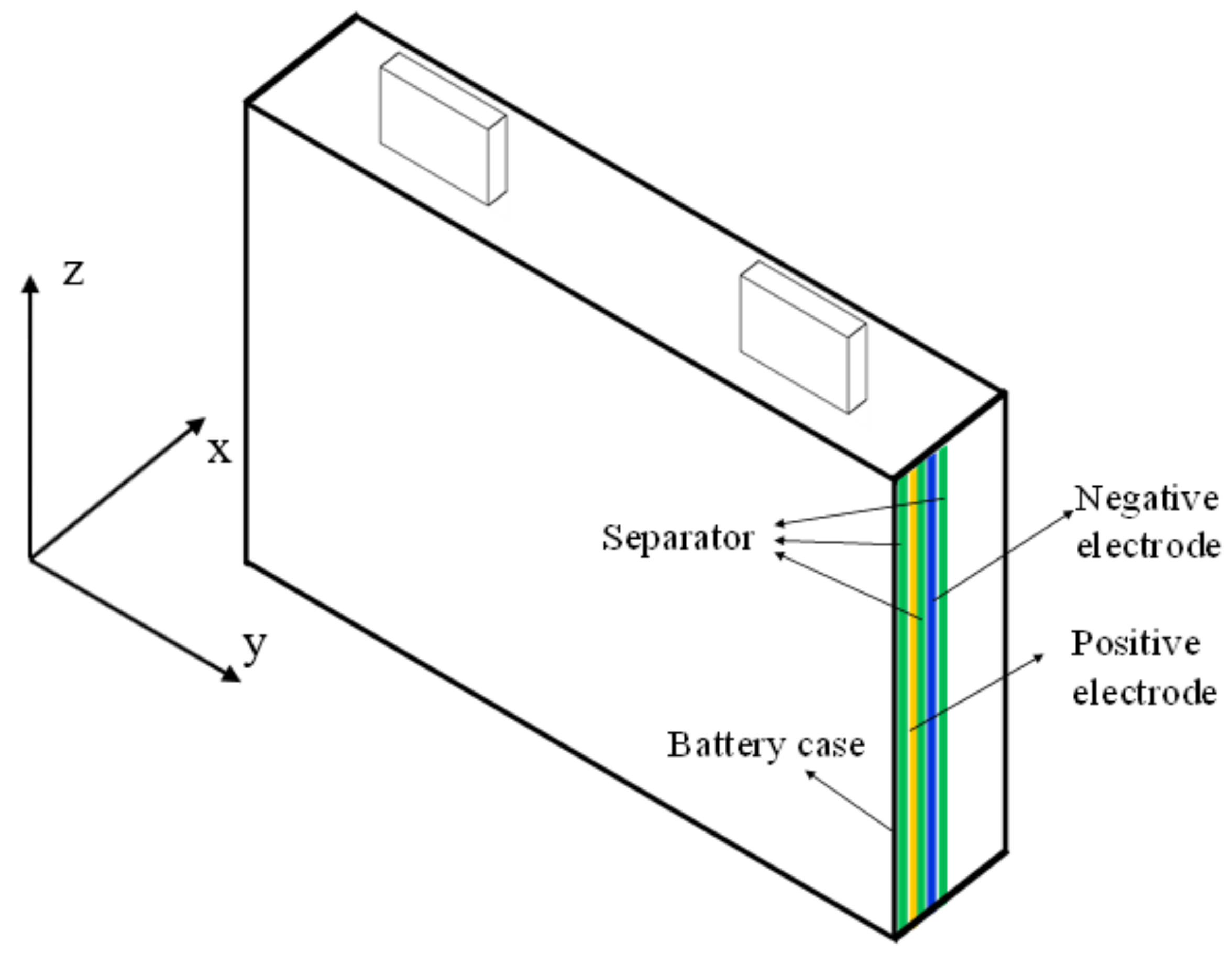
3. Electro-Thermal Model for Prismatic Cell

The model proposed in this work is a 0D/1D electro-thermal model, consisting of an equivalent circuit electrical model (ECM) and a lumped thermal model, as illustrated in Figure 2. The state of charge (SOC) was determined using the actual capacity, measured during the experimental campaign, along with the initial SOC. The electrical model takes as inputs the charge/discharge rate, temperature, and SOC, with the ECM parameters being extrapolated based on these three inputs. The outputs of the electrical model include terminal voltage and heat generation, the latter serving as an input for the lumped thermal model. At each time step t_i, the temperature (output of the thermal model) is computed and fed back into the electrical model to continue the calculation at the next time step t_i + Δt.

As will be shown in the following subsections, the model is based on analogies with electrical circuits; for this reason, it is not necessary to have a deep knowledge of internal cell phenomena such as diffusion and electrochemical and mass transport phenomena. The knowledge of these phenomena is, however, necessary in a physical–electrochemical model which results in a greater computational and modeling difficulty of much more complex phenomena than simple macroscopic phenomena, and with much longer computation times.

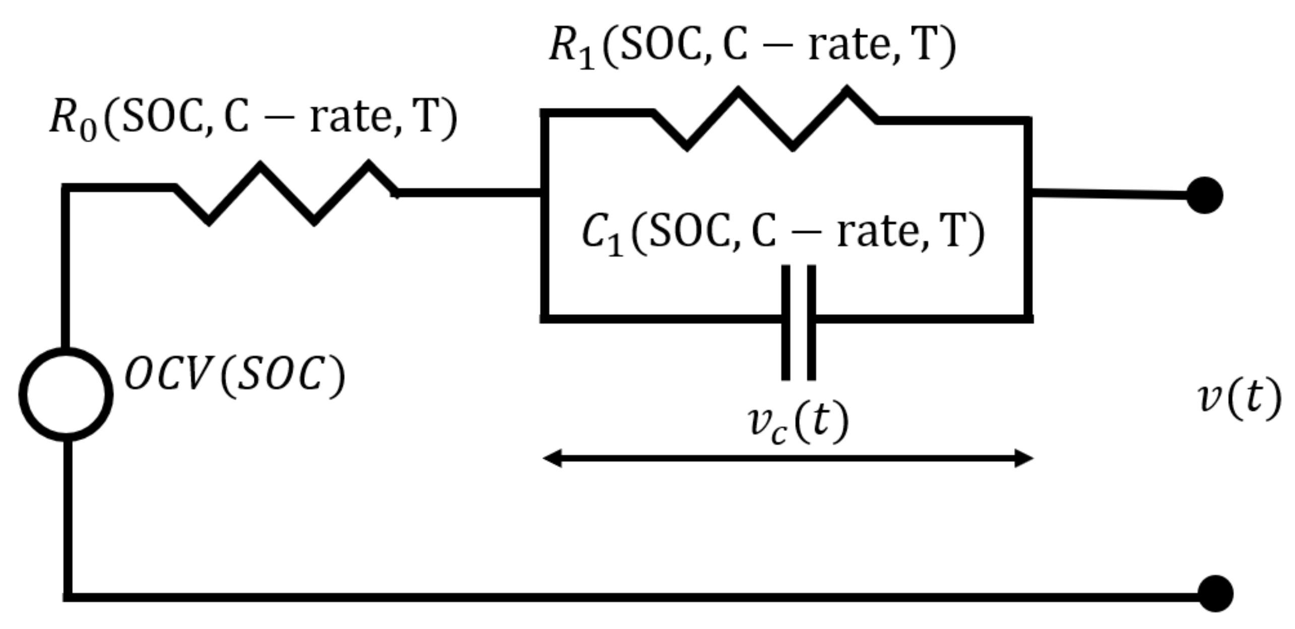
3.1. Electrical Model

An equivalent circuit model was employed in this work to represent the electrical behavior of the cell [26]. In this approach, the cell is modeled as an input/output system, where the input is the current, and the output is the voltage delivered at cell terminals [27].

A first order equivalent circuit model (Figure 3) was selected for this analysis. The main parameters calibrated for this model are as follows [28]:

The open circuit voltage source as a function of SOC: $\mathrm{O}\mathrm{C}\mathrm{V}=\mathrm{f}\left(\mathrm{S}\mathrm{O}\mathrm{C}\right)$. This represents the voltage that the cell delivers when it is unloaded and in a balanced condition. In this model, the OCV is considered to be a function of the state of charge (SOC). Several SOC estimation algorithms exist; in this study, the Coulomb counting method is used [29]:

$$SOC={SOC}_0-{\displaystyle \frac{1}{C_{Ah}}}{\int }_{t_0}^t\eta Idt$$

(1)

The accuracy of SOC estimation depends on the precision of both the previously mentioned parameters and the current sensor’s accuracy. The key parameters in the first-order equivalent circuit model include:

Ohmic resistance ${\mathrm{R}}_0=\mathrm{f}\left(\mathrm{S}\mathrm{O}\mathrm{C},\mathrm{c}-\mathrm{r}\mathrm{a}\mathrm{t}\mathrm{e},\mathrm{T},\mathrm{s}\mathrm{i}\mathrm{g}\mathrm{n}\left(\mathrm{I}\right)\right).$ This represents the instantaneous voltage drop that a cell experiences when connected to a load (or the voltage rise during charging). It accounts for ohmic losses occurring within the cell terminals and electrolyte [30];

The polarization resistance ${\mathrm{R}}_1=\mathrm{f}(\mathrm{S}\mathrm{O}\mathrm{C},\mathrm{c}-\mathrm{r}\mathrm{a}\mathrm{t}\mathrm{e},\mathrm{T},\mathrm{s}\mathrm{i}\mathrm{g}\mathrm{n}\left(\mathrm{I}\right))$ and the double-layer capacitance ${\mathrm{C}}_1=\mathrm{f}(\mathrm{S}\mathrm{O}\mathrm{C},\mathrm{c}-\mathrm{r}\mathrm{a}\mathrm{t}\mathrm{e},\mathrm{T},\mathrm{s}\mathrm{i}\mathrm{g}\mathrm{n}\left(\mathrm{I}\right))$. These parameters model the polarization losses inside the cell, which are caused by charge transfer and diffusion phenomena [30].

The equations used in the model are as follows [30]:

$$v\left(t\right)=OCV\left(SOC\left(t\right)\right)-v_c\left(t\right)-R_{0}I\left(t\right)$$

(2)

$${\displaystyle \frac{d{v}_c\left(t\right)}{dt}}={\displaystyle \frac{1}{C_1}}(I-{\displaystyle \frac{v_c\left(t\right)}{R_1}})$$

(3)

3.2. Heat Generation Model

Heat generation in a cell can be expressed as the sum of the following components [31]:

$$\dot{Q}=I·\left(V-OCV\right)+I·T{\displaystyle \frac{𝜕OCV}{𝜕T}}-{\sum }_i{∆H}_i^{avg}{s}_i-\int {\sum }_j\left(\overline{H_j}-{\overline{H_j}}^{avg}\right){\displaystyle \frac{𝜕f_j}{𝜕t}}du$$

(4)

Equation (4) on the right-hand side consists of four terms:

• Resistive heat generation: The first term represents the heat produced due to resistive dissipation. It is always positive and irreversible [32].
• Reversible entropic heat: The second term corresponds to entropic heat, which can be either positive or negative depending on the derivative of voltage with respect to temperature. This term was not considered in this study.
• Heat from chemical reactions: The third term accounts for the heat produced or absorbed during chemical reactions within the cell, which can also be positive or negative. This term was omitted from this work.
• Heat of mixing: This term arises from concentration gradients within the cell and is referred to as heat of mixing. This term was also removed from this study.

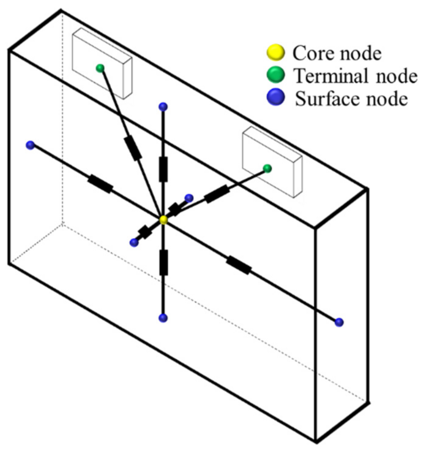
Thus, in this work, heat generation is simplified to the following form [33]:

$$\dot{Q}=I·\left(V-OCV\right)=I^2·R(SOC,T,I)$$

(5)

3.3. Thermal Model

A nodal network model was chosen to represent the thermal behavior of the cell in this analysis. This model is based on an electrical circuit analogy [34], where heat flow through nodes is analogous to current flow in an electrical circuit. There is a direct correlation between electrical current, driven by a voltage gradient, and heat transfer, driven by a temperature gradient. Each node in the model corresponds to a specific volume, composition, and thermal capacity. Inside the battery, heat is transferred between nodes via conduction, while at the external surfaces, heat dissipation occurs through convection, transferring heat from a surface node to the surrounding air. The only input to the model is heat generation (Equation (5)), which is estimated based on electrical parameters. Heat generation is distributed between the core and terminal nodes according to the allocation method proposed by Nazari et al. [31]. Radiation heat transfer was omitted from this study due to the low surface temperature of the cell.

The developed lumped thermal model for the prismatic cell is illustrated in Figure 4, consisting of nine internal cell nodes and one external node.

Core node: This node represents the active area inside the cell, specifically the jellyroll structure made up of several layers. The thermal capacity assigned to this node is calculated using average values of density and specific heat, considering the characteristics and dimensions of each layer.

Two terminal nodes: Each terminal is represented by a separate node.

Surface nodes: Each side wall of the cell is represented by a node.

Fluid node: This node represents the fluid surrounding the cell.

In this model, it is assumed that the heat flows from the innermost zone, the jellyroll, when it is produced due to ohmic effect and chemical reactions to the surfaces. Each surface is connected to the core by a conductive resistance; in the next section, the process of estimation of these conductive resistances is shown.

The thermal balance equation for a generic solid node, expressed in implicit form, can be written as follows [34]:

$$m_i{c}_i{\displaystyle \frac{T_{t+∆t}^i-T_t^i}{∆t}}={\sum }_j{K}_{ij}(T_{t+∆t}^j-T_{t+∆t}^i)+{\sum }_k{Q}_{k\to i}+{\sum }_j{h}_{ij}{A}_{ij}(T_f-T_{t+∆t}^i)$$

(6)

The advantage of the implicit formulation over the explicit method lies in its unconditional stability, making it particularly useful for simulating transient behavior, as is the case in this study. However, the implicit method is generally more computationally demanding.

By rearranging the thermal balance equations for all nodes in the analyzed system, a matrix expression is obtained [34]:

$$\left[T^t\right]={\left(\left[K\right]-\left[C\right]\right)}^{-1}(\left[T^{bc}\right]-[C][T^{t-∆t}])$$

(7)

For a steady-state problem, the transient term becomes zero, simplifying the thermal balance equation to Equation (8) [35]:

$$\left[T^t\right]={\left[K\right]}^{-1}\left[T^{bc}\right]$$

(8)

The identification of the thermal parameters included in the conductance and capacitance matrices is discussed in Section 4.4.

4. Parameter Identification

The parameters of the equivalent circuit model (ECM) were determined experimentally [35]. An experimental campaign was conducted to calibrate the parameters of a first-order equivalent circuit model under various environmental and operating conditions, including ambient temperature, discharge/charge rates, and state of charge (SOC) steps. The electrical parameters identified in the study include:

Cell capacity ${\mathrm{C}}_{\mathrm{A}\mathrm{h}}=\mathrm{f}(\mathrm{T},\mathrm{c}-\mathrm{r}\mathrm{a}\mathrm{t}\mathrm{e})$: Capacity affects SOC estimation (as shown in Equation (1)) and is expressed in Ah. It varies with temperature and electric current. To accurately map this parameter, capacity tests were conducted at different temperatures and discharge rates.

Open-circuit voltage $\mathrm{O}\mathrm{C}\mathrm{V}=\mathrm{f}\left(\mathrm{S}\mathrm{O}\mathrm{C}\right)$: OCV directly influences terminal voltage (as shown in Equation (2)). It was determined through OCV tests.

Resistances and capacitance ${\mathrm{R}}_0,{\mathrm{R}}_1,{\mathrm{C}}_1=\mathrm{f}(\mathrm{S}\mathrm{O}\mathrm{C},\mathrm{T},\mathrm{c}-\mathrm{r}\mathrm{a}\mathrm{t}\mathrm{e},\mathrm{s}\mathrm{i}\mathrm{g}\mathrm{n}\left(\mathrm{I}\right))$: ${\mathrm{R}}_0$ (Ohmic resistance), ${\mathrm{R}}_1$ (Polarization resistance), and ${\mathrm{C}}_1$ (Polarization capacitance) were determined using HPPC tests. These tests were conducted at various temperatures, charge/discharge rates, and SOC steps.

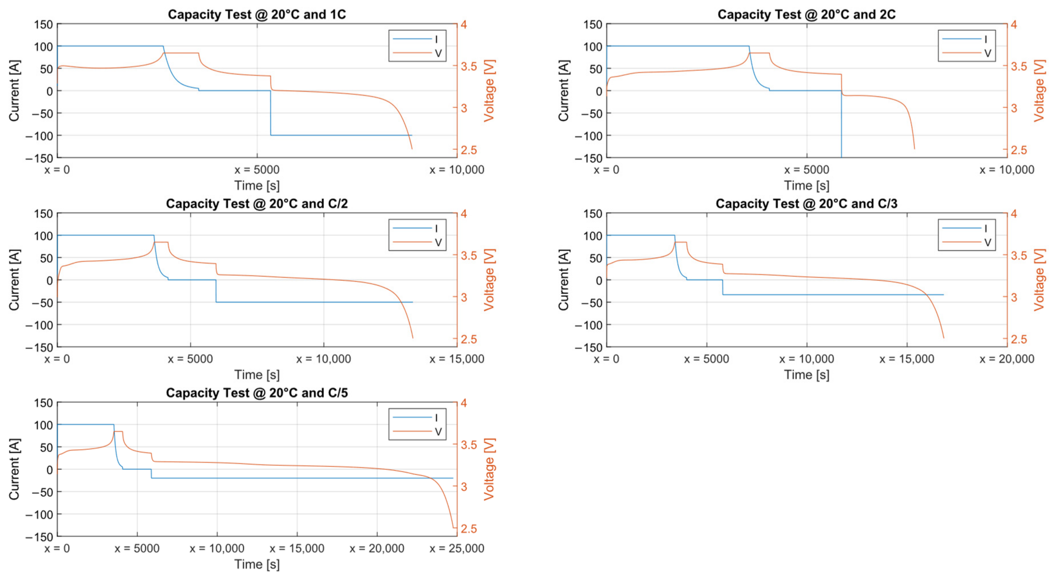
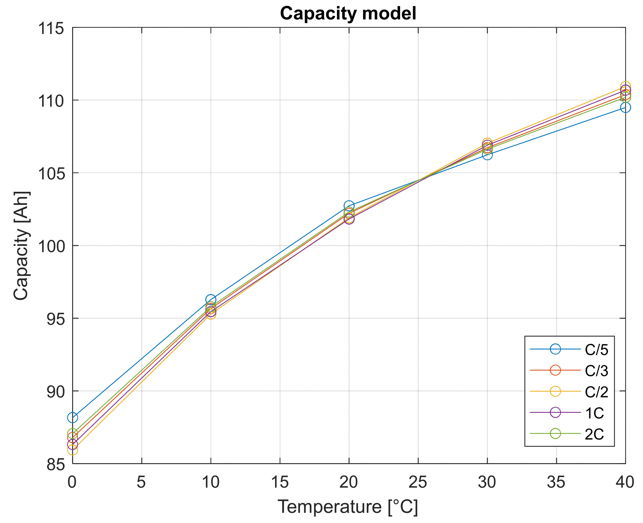
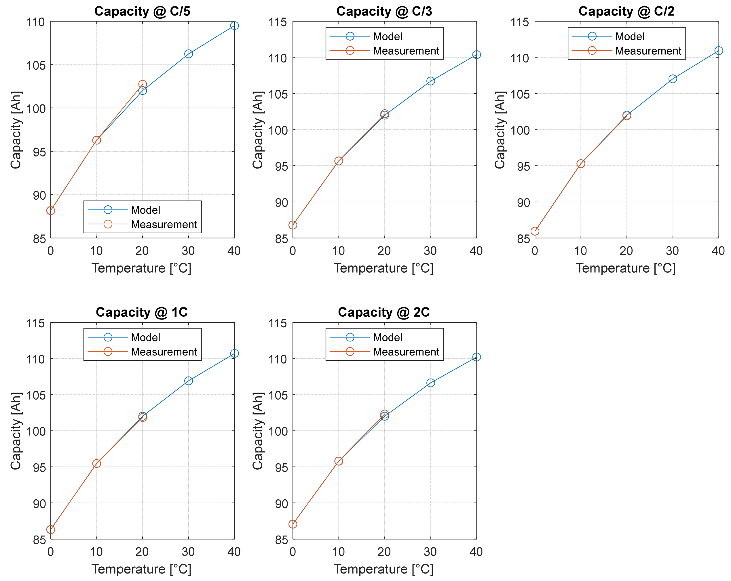
4.1. Capacity Identification

The capacity test protocol involves fully discharging the cell from its maximum voltage to the cutoff discharge voltage. The capacity test procedure for this cell includes:

Charging the cell using the CCCV protocol. The cell is charged at 1C until reaching the maximum voltage. The voltage is then maintained while the current decreases until a defined cutoff condition is met;

A rest period of half an hour;

Discharging the cell at the chosen rate.

This test was repeated at 5 discharge rates ($\mathrm{C}/5$, $\mathrm{C}/3$, $\mathrm{C}/2$, $1\mathrm{C}$, $2\mathrm{C}$) and three ambient temperatures ($0,10,\mathrm{a}\mathrm{n}\mathrm{d}20$°C). Figure 5 shows the capacity characterization campaign run at 20 °C for the prismatic cell.

The results of the capacity tests are summarized in Figure 6.

From Figure 6, it can be concluded that the capacity trend is influenced by two distinct phenomena: Peukert’s law and the self-heating effect. The capacity dependency on the discharge rate is evident, as described by Peukert’s law [36,37]. According to this law, higher discharge rates lead to lower available capacity, due to increased internal losses and inefficient charge utilization [38,39]:

$$I^{PC}·∆t=constant=C_n$$

(9)

where:

$∆\mathrm{t}$ is the time express in hours;

$\mathrm{P}\mathrm{C}$ is the Peukert Coefficient, which for lithium-ion cells is greater than 1 and it considers the losses happening inside the cell when it is discharging. These losses are higher when the cell is discharged at higher c-rates because the higher the c-rate is, the lower the number of active sites in the electrode is and, consequentially, the greater is the charge transfer resistance;

${\mathrm{C}}_{\mathrm{n}}$ is the nominal capacity, i.e., the capacity given by the manufacturer.

The observed capacity behavior is primarily influenced by diffusion phenomena occurring within the cell during charging and discharging: At higher temperatures, diffusion processes are enhanced, allowing a greater number of lithium-ions to migrate from the electrolyte to the electrode, leading to a higher effective capacity. Conversely, at lower temperatures, charge transfer resistance increases, meaning the resistance to ion flow through different cell phases is higher, which reduces the available capacity. Due to self-heating, a cell operating at higher discharge rates can experience a temperature rise. As a result, this thermal effect can counteract capacity losses by improving diffusion kinetics, leading to a capacity increase at high discharge rates.

To calibrate cell capacity beyond the conditions tested in the experimental matrix, the model proposed by Galushkin et al. [39] was considered. The Galushkin model is used for capacity–temperature dependency because as it provides a physically motivated representation of diffusion-based processes in lithium-ion batteries, making it more suitable than conventional empirical curve-fitting models:

$$C=C_n{K}_{cap}·{\displaystyle \frac{{(\frac{T-T_0}{T_{ref}-T_0})}^{\beta }}{\left(K_{cap}-1\right)+{(\frac{T-T_0}{T_{ref}-T_0})}^{\beta }}}$$

(10)

This physical extrapolation model, once the tuning parameters ${\mathrm{K}}_{\mathrm{c}\mathrm{a}\mathrm{p}}$ and $\mathsf{\beta }$ are calibrated, allows the determination of capacity values at temperature other than the test matrix’s. The results of Galushkin model calibration for the cell object of this study are shown in Figure 7.

The agreement between the capacity values obtained from the experimental campaign and the values obtained from the physical extrapolation model is shown in Figure 8. This model allows for a precise estimation of cell capacity at temperatures other than those tested. The agreement between the model and the measurement is expressed in term of ${\mathrm{R}}^2$ and the results are shown in

Table 2. Precision of the Galushkin extrapolation model.

C-Rate	C/5	C/3	C/2	1C	2C
$R^2$	0.9973	0.9992	0.996	0.9993	0.9989

.

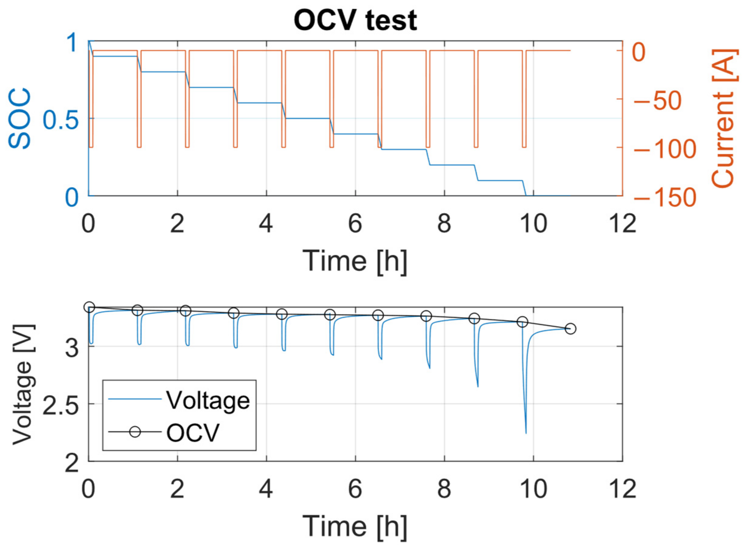
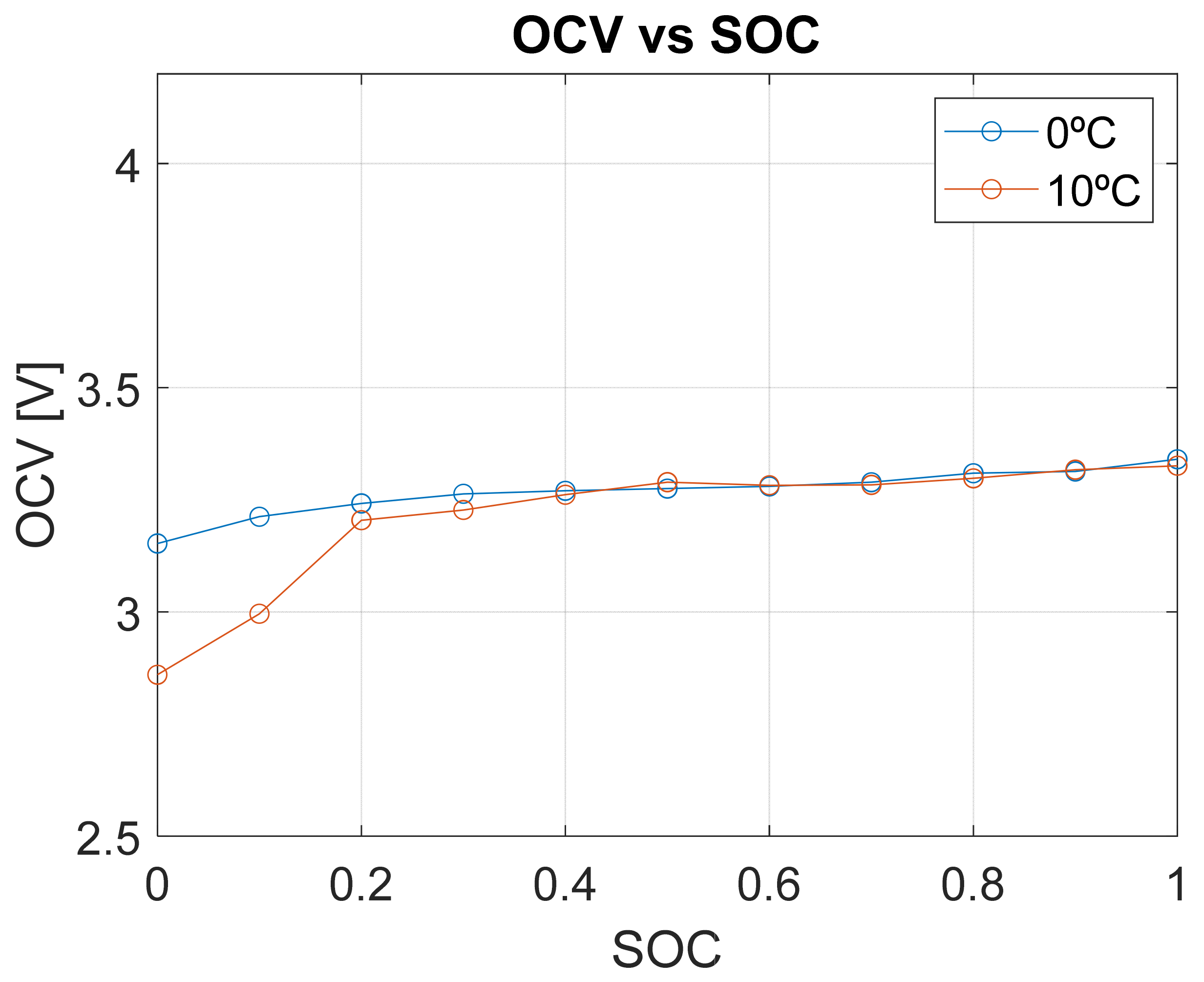
4.2. OCV Identification

To determine the open circuit voltage, several OCV test [40] were conducted at different temperatures. Various procedures for OCV testing are described in the literature [41], but typically, the process involves fully charging the cell according to the CCCV protocol at 1C, followed by a 1 to 3 h rest period. Next, a series of 10% discharge cycles is performed, each followed by a 1 to 3 h rest period, until the battery is fully discharged. Similarly, the recharge process is carried out by alternating 10% charging cycles with 3 h rest periods until the cell reaches full charge. The open-circuit voltage (OCV) curve is constructed using the voltage values recorded at the end of each rest period, as it is assumed that the voltage stabilizes after a sufficiently long rest. Figure 9 illustrates the OCV test conducted in this study, showing the voltage stabilization behavior and how the OCV curve is determined.

From Figure 9, it is evident that the lower is the state of charge, the lower is the open circuit voltage. The OCV decreases with respect to the SOC in an almost linear way from a fully charged condition to approximately 20% of the SOC [42], and then, it decreases rapidly to its minimum at 0% of the SOC [43].

Although the open-circuit voltage (OCV) is largely independent of temperature, the experimental data in Figure 10 reveal that at low state-of-charge (SOC < 0.2), temperature does influence the OCV. This temperature dependency at low SOC levels has been widely reported in the literature and is attributed to electrochemical and thermodynamic effects within the cell. At low SOC, variations in lithium-ion concentration, electrode surface reactions, and electrolyte properties can lead to OCV fluctuations depending on temperature conditions [43].

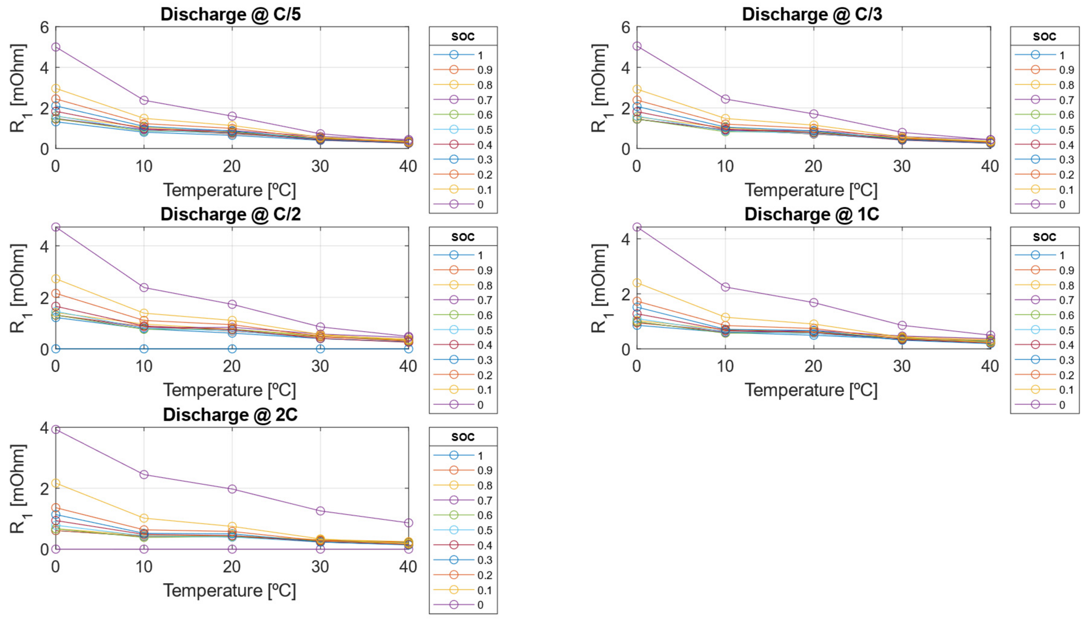
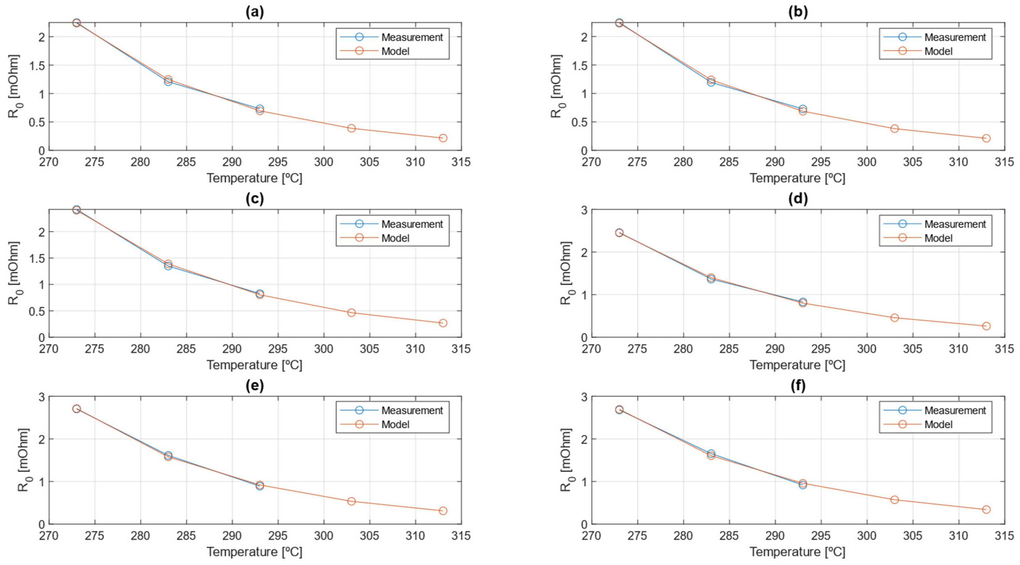
4.3. Electrical Parameters Identification: $R_0,R_1,C_1$

The electrical parameters for the first-order equivalent circuit model were determined using the Hybrid Pulse Power Characterization (HPPC) test [44], as described in the Idaho National Laboratory manual. However, this study employed a modified protocol. While the standard HPPC test evaluates the cell’s behavior only at 1C, the adapted approach enables a multi-rate analysis, providing a more comprehensive understanding of the battery’s characteristics.

The HPPC protocol used in this work consists of the following steps, as shown in Figure 11:

• Initial charge at 1C following the CCCV protocol;
• One-hour rest period;
• 10% discharge of the cell capacity at 1C;
• One-hour rest period;
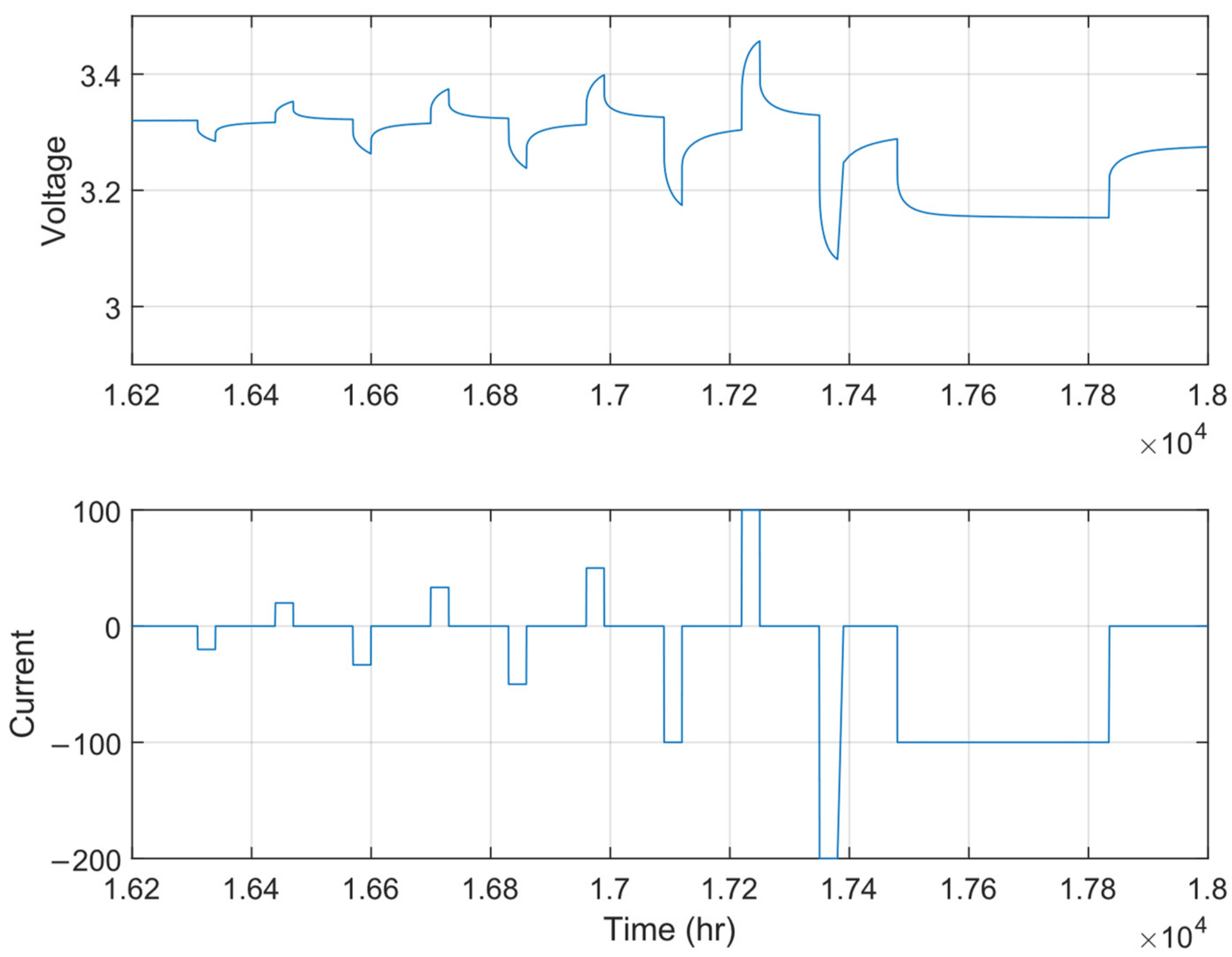
• Application of a pulse train at the corresponding SOC level: Discharge pulses at C/5, C/3, C/2, 1C; charge pulses at C/5, C/3, C/2, and 1C. The pulse train is illustrated in Figure 12.

Steps 3 to 5 are repeated until the cell is fully discharged. The tests were performed at 0 °C, 10 °C, and 20 °C. The main difference with respect to the HPPC test protocol described in [45] is the fact that, in this work, a protocol with several pulses in charge and discharge is proposed, while the original protocol considers only a pulse at 1C. This aspect allows for a more complete understanding of how electrical parameters vary with respect to the charge/discharge rate and for a better estimation of the heat generation.

Once the test is run, the electrical parameters are obtained through a calibration method called the step-method. This is based on the fact that ${\mathrm{R}}_0$ models the instantaneous variation in the voltage response (Figure 13) and an initial value can be estimated considering the instantaneous voltage variation (points 0 and 1) over instantaneous current variation; ${\mathrm{R}}_1$ models the resistance caused by the charge transfer process from electrolyte to electrode and it is calibrated considering the exponential voltage variation, and ${\mathrm{C}}_1$ is the double-layer capacitance. These two parameters characterize the cell’s dynamic behavior, specifically the voltage variation during the current pulse. Consequently, their initial values are determined by the pulse voltage variation (points 1 and 2) relative to the instantaneous current variation. Therefore, the initial values for the optimization process are determined using the following expressions [45,46]:

$$R_{0,in}={\displaystyle \frac{v_1-v_0}{I_1-I_0}}$$

(11)

$$R_{tot}={\displaystyle \frac{v_2-v_0}{I_2-I_0}}={\displaystyle \frac{v_2-v_0}{I_1-I_0}}$$

(12)

$$R_{1,in}=R_{tot}-R_{0,in}=\left|{\displaystyle \frac{v_2-v_1}{I_2-I_0}}\right|$$

(13)

$${\tau }_{RC}=t_2-t_1=R_{1,in}{C}_{1,in}\to C_{1,in}={\displaystyle \frac{{\tau }_{RC}}{R_{1,in}}}$$

(14)

Once the initial guess values are obtained, they are optimized to ensure a close agreement between the model and the experimental data. The function that is minimized is the error (Equation (15)) between the modeled voltage drop (Equations (16) and (17)) and the experimental voltage drop:

$$err=\sqrt{{\displaystyle \frac{1}{t_{pulse}}}{\sum }_{i=1}^{t_{pulse}}{(v_{mod,i}-v_{exp,i})}^2}$$

(15)

$$v_{mod,i}=OCV-v_{c,OPT}\left(t\right)-R_{0,OPT}I\left(t\right)$$

(16)

$${\displaystyle \frac{d{v}_{c,OPT}\left(t\right)}{dt}}={\displaystyle \frac{1}{C_{1,OPT}}}(I-{\displaystyle \frac{v_{c,OPT}\left(t\right)}{R_{1,OPT}}})$$

(17)

The electrical parameters experimentally calibrated in this work are shown in Figure 14, Figure 15 and Figure 16.

The electrical resistances decrease as the C-rate increases but also decrease as the SOC decreases. This behavior arises because, as the cell approaches a fully discharged state, ion migration from the electrode to the liquid phase becomes more challenging due to the worsening of diffusion and mass transport phenomena within the cell. Conversely, the double-layer capacitance increases with higher C-rates but decreases as SOC decreases. As shown in Figure 17 and Figure 18, the resistive parameters—both ohmic resistance and charge transfer resistance—exhibit an Arrhenius-type dependency on temperature. This temperature dependence is well-documented in the literature, confirming the observed trends [47,48].

$$R_i=A_f{e}^{-{\displaystyle \frac{E_a}{R_{gas}T}}}$$

(18)

Once the pre-exponential factor and activation energy are calibrated, the Arrhenius-like model is employed to extrapolate electrical parameter values at temperatures beyond those measured experimentally. The Arrhenius model is specifically chosen for resistance estimation due to its well-established foundation in thermally activated processes that govern charge transport and reaction kinetics. Compared to simple linear approximations, this model offers a more robust and physically meaningful framework, ensuring greater accuracy in capturing the temperature dependence of electrical resistance in lithium-ion batteries. This allows to have an estimation of electrical parameters outside the considered test matrix, i.e., to reduce testing and calibration time for the use of the model. In Figure 17 and Figure 18, the calibrated ohmic resistance R₀ and the charge transfer resistance R₁ obtained using a physics-based approach, are presented. Figure 18 provides valuable insights into the ideal SOC operating range, reinforcing the importance of limiting Depth of Discharge to optimize battery longevity and performance.

As for the capacity extrapolation model, also for the Arrhenius extrapolation model, the agreement between parameters estimated from the experimental data and parameters obtained with the extrapolation model is provided for the ohmic resistance in Figure 19.

This agreement is shown for a particular condition, given the huge amount of data: the results are shown for 1C pulses in discharge and charge and with $\mathrm{S}\mathrm{O}\mathrm{C}=\left[10.50\right]$, that are, respectively, fully charged condition, half charged condition, and fully discharged condition. Also, in this case, the indicator ${\mathrm{R}}^2$ is provided as an indicator of the precision of the extrapolation model with respect to the data from post-processing, as shown in

Table 3. Precision of the Arrhenius extrapolation model.

1C Charge	$\mathit{S}\mathit{O}\mathit{C} = 1$	$\mathit{S}\mathit{O}\mathit{C} = 0.5$	$\mathit{S}\mathit{O}\mathit{C} = 0$
$R^2$	0.9994	0.9992	0.9996
1C Discharge	$SOC=1$	$SOC=0.5$	$SOC=0$
$R^2$	0.9996	0.9997	0.9998

.

4.4. Thermal Parameter Identification

The parameters required for the calibration of the thermal model are as follows:

-

Thermal capacity of the cell;

-

Internal conductive resistances between nodes;

-

External convective resistances with air.

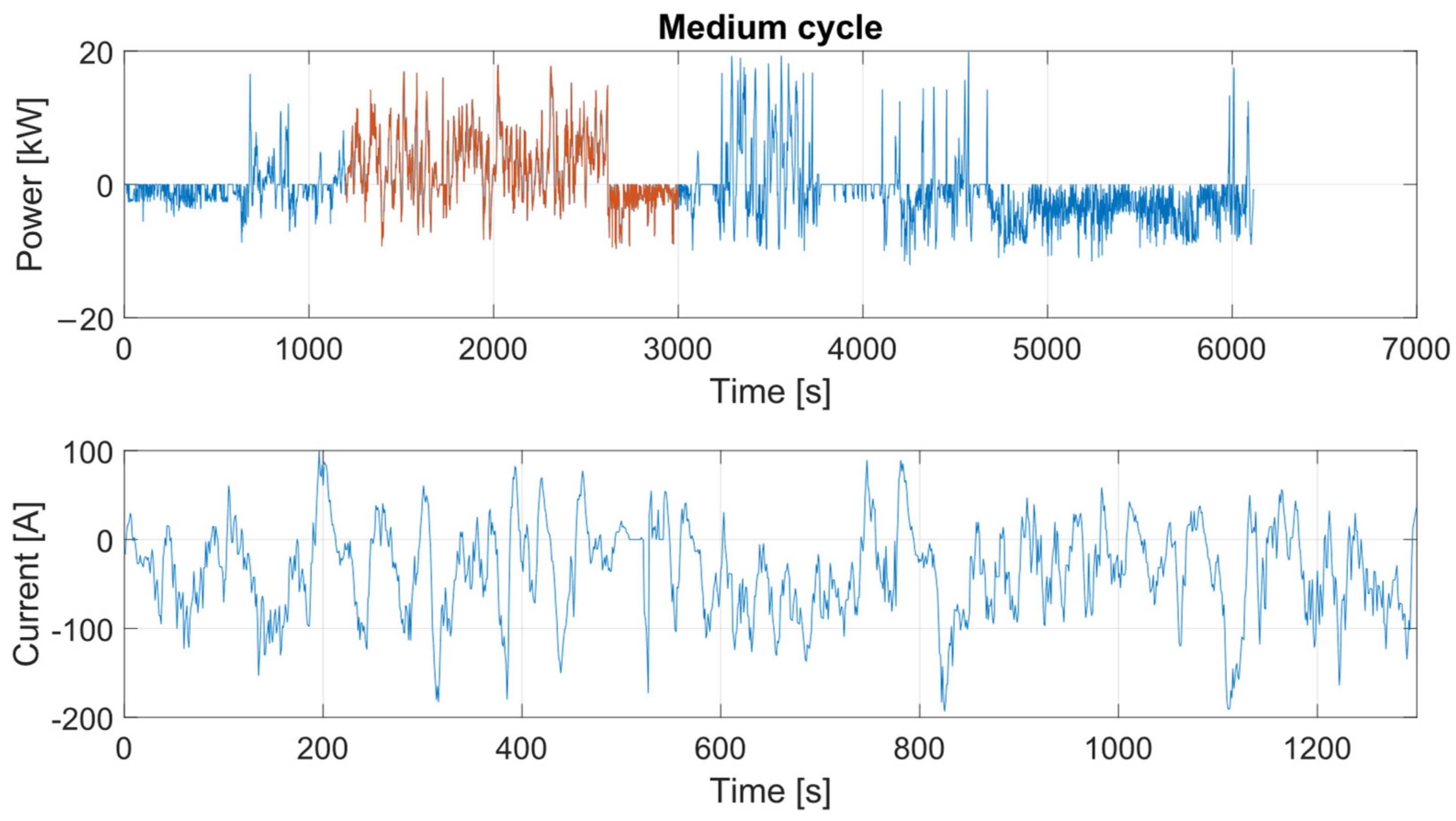
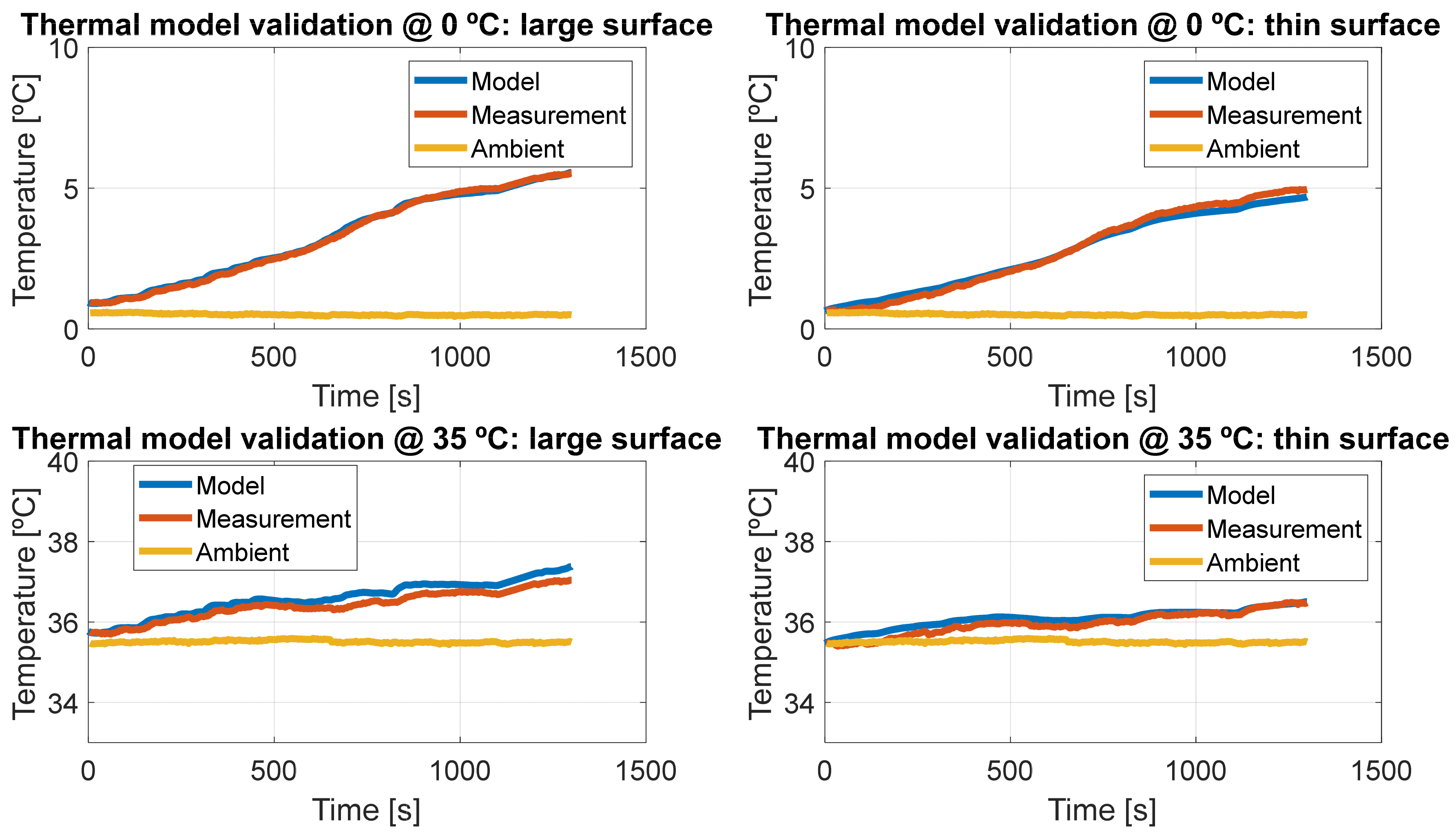
These parameters were determined based on the cell’s internal geometric properties and thermal characteristics obtained from the literature.

To determine the thermal capacity of the cell, average density and average specific heat must be determined. Given that the internal structure of the prismatic cell consists of a jellyroll composed of multiple layers, as illustrated in Figure 20, it is essential to determine the characteristics of each layer, which are listed in

Table 4. Thermal characteristics of the jellyroll materials.

	Material	Specific Heat $[\mathbf{J}·{\mathbf{k}\mathbf{g}}^{-1}·{\mathbf{K}}^{-1}]$	Density $[\mathbf{k}\mathbf{g}·{\mathbf{m}}^{-3}]$
Positive current collector	Aluminum	903	2700
Cathode Electrode	LFP	1260.2	1500
Separator	PP/PE/PP	1978	492
Anode electrode	Graphite	1437.4	2660
Negative current collector	Copper	385	8900

[49,50].

Finally, the thermal capacity, knowing all the characteristics of each of the layers composing the jellyroll of the cell, is calculated, as shown in Figure 20.

Regarding the calculation of internal conductive resistances and based on the findings of Xie et al. [30], the average thermal conductivity can be estimated by considering key internal characteristics of the cell, such as the porosity of the layers, the thermal conductivity of the electrolyte, and the thermal conductivity of the jellyroll layers. Following the methodology presented in various studies, the thermal conductivity of each layer, when soaked in the electrolyte, can be determined using the following approach [51]:

$$k_i=k_m·\left(1-\epsilon \right)+k_{el}·\epsilon$$

(19)

Since the thermal conductivity of each layer has been determined, it is now possible to compute the overall thermal conductivity along different axes of the cell [51]:

$$k_x={\displaystyle \frac{L_x}{{\sum }_{i=1}^N\frac{L_{x,i}}{k_i}}}={\displaystyle \frac{1}{{\sum }_{i=1}^N\frac{{\delta }_i}{k_i}}}$$

(20)

$$k_y=k_z={\sum }_{i=1}^N{\displaystyle \frac{L_{x,i}{k}_i}{L_x}}={\sum }_{i=1}^N{\delta }_i{k}_i$$

(21)

5. Model Validation

Once all the parameters of the electro-thermal model were determined—either experimentally or through reference values from the scientific literature—the model was validated using an in-house real driving emissions (RDEs) cycle, designed in compliance with current regulations [52]. In particular, the profile, shown in Figure 21, represents a power profile with which the battery is charged and discharged.

For this power profile, for validation purposes, an interval of 1400 s was selected, and it was converted into an electric current. This RDEs cycle was implemented in the bidirectional source software and, in this way, the cell was loaded and unloaded.

Figure 22 presents the validation results of the electrical model by comparing the simulated voltage signal at the cell terminals with the measurements obtained from the bidirectional source. Additionally, it validates the thermal model by comparing the simulated temperatures with those measured by two K-type thermocouples placed on the surface of the prismatic cell.

The validation of the electro-thermal model demonstrates that it accurately captures both the overall trend and the instantaneous variations in both the electrical and thermal domains. The agreement between the model and experimental measurements is quantified using the root mean square error (RMSE), as shown below:

$${rmse}_{electrical}={\displaystyle \frac{\sqrt{\frac{1}{n_1}{\sum }_{i=1}^{n_1}{(v_{mod}-v_{exp})}^2}}{mean\left(v_{exp}\right)}}·100=0.54\%$$

(22)

$${rmse}_{thermal,largsurf}={\displaystyle \frac{\sqrt{\frac{1}{n_2}{\sum }_{i=1}^{n_2}{(T_{ls,mod}-T_{ls,exp})}^2}}{mean\left(T_{ls,exp}\right)}}·100=0.86\%$$

(23)

$${rmse}_{thermal,thinsurf}={\displaystyle \frac{\sqrt{\frac{1}{n_3}{\sum }_{i=1}^{n_3}{{(T}_{ts,mod}-T_{ts,exp})}^2}}{mean\left(T_{ts,exp}\right)}}·100=0.33\%$$

(24)

The same validation cycle was used for a multi-temperature validation of the model. The cell was tested under cold climate conditions (0 °C) and very hot climate conditions (35 °C) to assess its accuracy across a wide temperature range.

The results of the validation at the other temperatures are shown in Figure 23.

The model demonstrates strong agreement across all tested ambient temperature conditions. As expected, at lower temperatures, the internal resistance of the cell increases, leading to greater temperature rises at 0 °C compared to 35 °C. This behavior is consistent with the well-known thermal and electrical properties of lithium-ion cells. The RMS errors for both 0 °C and 35 °C cases are presented in

Table 5. RMSE of the model at 0 and 35 °C.

	0 °C	35 °C
${rmse}_{thermal,largsurf}[\%]$	$0.86\%$	$0.55\%$
${rmse}_{thermal,thinsurf}[\%]$	$0.60\%$	$0.38\%$

.

Nonetheless, despite the fact that no experimental calibration was carried out at a higher temperature than 20 °C, the model shows a good agreement with experimental measurement, proving the goodness of the coupling with the Galushkin and Arrhenius extrapolation models.

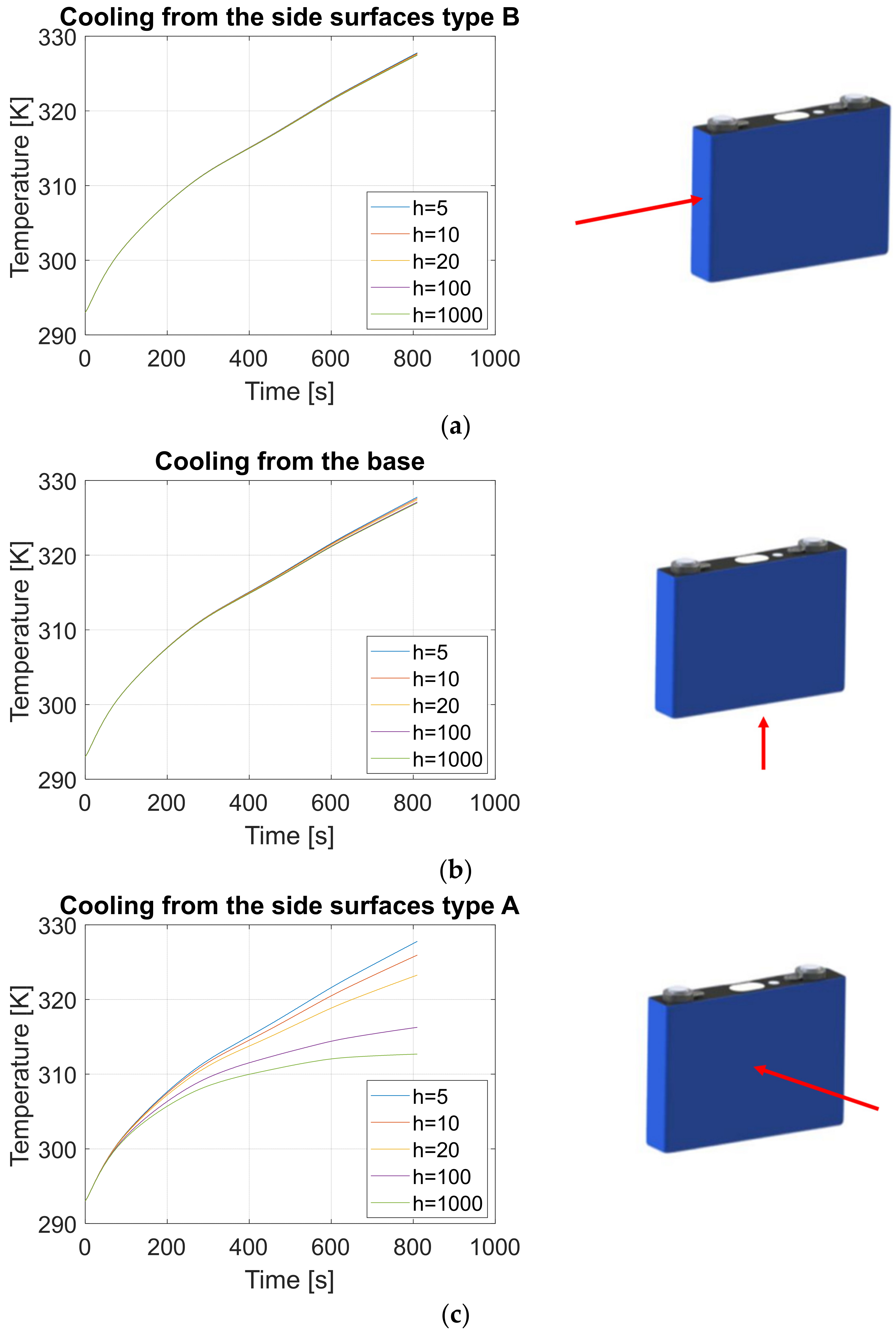
6. Cooling Strategies Analysis

One of the most extensively studied topics in the literature on lithium-ion battery pack technologies is thermal management systems and their comparative analysis [53]. In this section, this topic is examined using the calibrated and validated computational tools developed in the previous sections.

The objective of this analysis is to evaluate the impact of varying the heat transfer coefficient at the base or lateral surfaces on the core temperature of the cell. This study assumes a 4C charge rate (400 A for this cell), representing a fast-charging scenario in which the cell is fully recharged within 15 min.

The heat transfer coefficient varied from 5 W/m²·K to 1000 W/m²·K, covering a range that corresponds to typical cooling methods, including free convection in air, forced convection in air, and liquid cooling.

Three possible cell cooling configurations were considered:

• From the side surfaces type B (see Figure 24);
• From the base;
• From the side surfaces type A (see Figure 24).

Figure 24 presents the results of 15 simulations, with 5 simulations for each of the three cell cooling strategies during a 4C charge. The plotted temperatures represent the core temperature of the cell, which is assumed to be the hottest region where heat is generated due to both reversible and irreversible effects.

The model produces results that align with expected thermal behavior for the analyzed cooling strategies:

-

Natural convection with air (h = 5–10 W/m²·K) shows minimal impact on cooling, regardless of the cooling strategy. In all three cases, the temperature evolution remains nearly identical within this low heat transfer coefficient range.

-

Liquid cooling (h = 100–1000 W/m²·K) demonstrates a significant improvement in cooling performance. The model indicates that cooling from the side B walls is more effective than cooling from the base or other side walls, leading to superior heat dissipation and lower core temperatures.

These results emphasize the importance of cooling placement and highlight the efficiency of side-wall cooling in managing temperature rise during high C-rate charging scenarios.

In this analysis, the parameter considered in order to estimate the goodness of the cooling strategy is the temperature difference at the end of the charging process (after approximately 800 s) between the case with a heat exchange coefficient equal to $5\mathrm{W}/{\mathrm{m}}^2\mathrm{K}$ (natural convection) and the case in which the heat exchange coefficient is equal to $1000\mathrm{W}/{\mathrm{m}}^2\mathrm{K}$ (liquid cooling strategy).

This coefficient is expressed in percentage with respect to the temperature variation that occurs in the cell in the worst-case scenario, that is, when the heat transfer coefficient is equal to $5\mathrm{W}/{\mathrm{m}}^2\mathrm{K}$:

$${∆T}_{sideB}={\displaystyle \frac{{∆T}_{sideB}\left(t=t_{end};h=5\right)-{∆T}_{sideB}\left(t=t_{end};h=1000\right)}{{∆T}_{sideB}\left(t=t_{end};h=5\right)-{∆T}_{sideB}\left(t=t_0;h=5\right)}}·100=1\%$$

(25)

$${∆T}_{base}={\displaystyle \frac{{∆T}_{base}\left(t=t_{end};h=5\right)-{∆T}_{base}\left(t=t_{end};h=1000\right)}{{∆T}_{base}\left(t=t_{end};h=5\right)-{∆T}_{base}\left(t=t_0;h=5\right)}}·100=2\%$$

(26)

$${∆T}_{sideA}={\displaystyle \frac{{∆T}_{sideA}\left(t=t_{end};h=5\right)-{∆T}_{sideA}\left(t=t_{end};h=1000\right)}{{∆T}_{sideA}\left(t=t_{end};h=5\right)-{∆T}_{sideA}\left(t=t_0;h=5\right)}}·100=43\%$$

(27)

Equations (25)–(27) allow further considerations to be made:

If the cell is cooled from its side B walls or from the base, the increase of heat transfer coefficient does not have a considerable impact. This is because the maximum temperature reached during charging operations in free convection in air ($\mathrm{h}=5\mathrm{W}·{\mathrm{m}}^{-2}{\mathrm{K}}^{-1})$ and the forced convection with liquid ($\mathrm{h}=1000\mathrm{W}·{\mathrm{m}}^{-2}{\mathrm{K}}^{-1})$ is neglectable, compared to the temperature difference during entire charging operations in the worst-case scenario. In fact, this coefficient is equal to 1% for side B cooling and to 2% for base cooling.

If the cell is cooled from its side A walls, the increase of heat transfer coefficient leads to a global improvement in cooling operations. The abovementioned parameter is, in fact, equal to 43%: this means that cooling with liquid ($\mathrm{h}=1000\mathrm{W}·{\mathrm{m}}^{-2}{\mathrm{K}}^{-1})$ allows for, in this case, a great reduction in the maximum temperature reached by the cell during charging operations and this is very important as soon as the rate of charge of the battery increases.

In

Table 6. Cooling strategy analysis results.

	h = $10\mathbf{W}·{\mathbf{m}}^{-2}{\mathbf{K}}^{-1}$	h = $20\mathbf{W}·{\mathbf{m}}^{-2}{\mathbf{K}}^{-1}$	h = $50\mathbf{W}·{\mathbf{m}}^{-2}{\mathbf{K}}^{-1}$	h = $100\mathbf{W}·{\mathbf{m}}^{-2}{\mathbf{K}}^{-1}$	h = $1000\mathbf{W}·{\mathbf{m}}^{-2}{\mathbf{K}}^{-1}$
Side B cooling	54.78 °C	54.70 °C	54.61 °C	54.50 °C	54.46 °C
Base cooling	54.78 °C	54.61 °C	54.42 °C	54.12 °C	54.00 °C
Side A cooling	54.78 °C	52.95 °C	50.27 °C	43.27 °C	39.69 °C
Temperature decrease of side A cooling with respect of side B cooling [%]	0	−3.30	−8.64	−25.94	−37.23
Temperature decrease of side A cooling with respect of base cooling [%]	0	−3.15	−8.27	−25.06	−36.07

, the temperature at the end of each charging process is shown for each of the cooling configurations analyzed. Furthermore, percentage temperature decrease of the optimal solution (side A cooling) with respect to the base and side B cooling is shown. Overall, in conditions of convection with liquid ($\mathrm{h}>100\mathrm{W}·{\mathrm{m}}^{-2}{\mathrm{K}}^{-1})$, the advantage in side A cooling is very relevant if compared to side B or base cooling.

7. Conclusions

This study presents an electro-thermal model for a prismatic lithium-ion battery. The model consists of the following:

-

A first-order equivalent circuit model, with parameters calibrated through an experimental campaign.

-

A nodal thermal model, where parameters are estimated based on the internal structure of the cell, assigning specific density, specific heat capacity, and thermal conductivity values to each material, and then calculating the global thermal properties of the cell.

The main advantages of the model are as follows:

-

Low computational cost, making it efficient for practical applications.

-

No requirement for detailed knowledge of internal battery phenomena such as diffusion, mass transport, or electrochemical reactions, simplifying both calibration and usage.

-

Scalability: the proposed methodology for experimental characterization and modeling can be applied to any prismatic cell, regardless of its chemistry or geometry.

To minimize the required test matrix, two physics-based extrapolation models were integrated. This allowed for parameter estimation beyond the experimental temperature range. In this case, a three-temperature characterization campaign was conducted, and parameters were extrapolated to higher temperatures.

The model was validated under dynamic conditions, demonstrating strong agreement with experimental measurements in both the electrical and thermal domains. The validation was performed at three temperature conditions (cold, mild, and hot), ensuring accuracy over a broad temperature range. The maximum error remained below 1% across all thermal measurements at different ambient temperatures.

This study also examined various cooling strategies for a prismatic cell, revealing that the most effective method is lateral liquid cooling. Base cooling provides limited benefits in reducing temperature and mitigating the risk of thermal runaway during ultra-fast charging. Side cooling can reduce the maximum cell temperature by up to 36% compared to base cooling, making it the preferred solution.

A potential future development would be to extend the analysis from a single cell to a full battery pack and integrate the electro-thermal model with a thermo-hydraulic model that accounts for the effects of a thermal management system.

References

1. Muratori, M.; Alexander, M.; Arent, D.; Bazilian, M.; Cazzola, P.; Dede, E.M.; Farrell, J.; Gearhart, C.; Greene, D.; Jenn, A.; et al. The rise of electric vehicles—2020 status and future expectations. Prog. Energy 2021, 3, 022002. [Google Scholar] [CrossRef]
2. Rajashekara, K. Present status and future trends in electric vehicle propulsion technologies. IEEE J. Emerg. Sel. Top. Power Electron. 2013, 1, 3–10. [Google Scholar] [CrossRef]
3. Zubi, G.; Dufo-López, R.; Carvalho, M.; Pasaoglu, G. The lithium-ion battery: State of the art and future perspectives. Renew. Sustain. Energy Rev. 2018, 89, 292–308. [Google Scholar] [CrossRef]
4. Lebedeva, N.; Di Persio, F.; Boon-Brett, L. Lithium Ion Battery Value Chain and Related Opportunities for Europe; European Commission: Petten, The Netherlands, 2016. [Google Scholar]
5. Un-Noor, F.; Padmanaban, S.; Mihet-Popa, L.; Mollah, M.N.; Hossain, E. A comprehensive study of key electric vehicle (EV) components, technologies, challenges, impacts, and future direction of development. Energies 2017, 10, 1217. [Google Scholar] [CrossRef]
6. Scrosati, B.; Hassoun, J.; Sun, Y.K. Lithium-ion batteries. A look into the future. Energy Environ. Sci. 2011, 4, 3287–3295. [Google Scholar] [CrossRef]
7. Anderson, D. An Evaluation of Current and Future Costs for Lithium-Ion Batteries for Use in Electrified Vehicle Powertrains. Master’s Thesis, Nicholas School of the Environment of Duke University, Durham, NC, USA, 2009. [Google Scholar]
8. Agwu, D.; Opara, F.; Chukwuchekwa, N.; Dike, D.; Uzoechi, L. Review of Comparative Battery Energy Storage System (BESS) for Energy Storage Applications in Tropical Environment. In Proceedings of the IEEE 3rd International Conference on Electro-Technology for National Development, Owerri, Nigeria, 7–10 November 2017. [Google Scholar]
9. Bandhauer, T.M.; Garimella, S.; Fuller, T.F. A critical review of thermal issues in lithium-ion batteries. J. Electrochem. Soc. 2011, 158, R1. [Google Scholar] [CrossRef]
10. Wang, Q.; Ping, P.; Zhao, X.; Chu, G.; Sun, J.; Chen, C. Thermal runaway caused fire and explosion of lithium ion battery. J. Power Sources 2012, 208, 210–224. [Google Scholar] [CrossRef]
11. Feng, X.; Ouyang, M.; Liu, X.; Lu, L.; Xia, Y.; He, X. Thermal runaway mechanism of lithium ion battery for electric vehicles: A review. Energy Storage Mater. 2018, 10, 246–267. [Google Scholar] [CrossRef]
12. Wu, W.; Ma, R.; Liu, J.; Liu, M.; Wang, W.; Wang, Q. Impact of low temperature and charge profile on the aging of lithium-ion battery: Non-invasive and post-mortem analysis. Int. J. Heat Mass Transf. 2021, 170, 121024. [Google Scholar] [CrossRef]
13. Gao, S.; Feng, X.; Lu, L.; Kamyab, N.; Du, J.; Coman, P.; White, R.E.; Ouyang, M. An experimental and analytical study of thermal runaway propagation in a large format lithium ion battery module with NCM pouch-cells in parallel. Int. J. Heat Mass Transf. 2019, 135, 93–103. [Google Scholar] [CrossRef]
14. He, C.; Yue, Q.; Wu, M.; Chen, Q.; Zhao, T. A 3D electrochemical-thermal coupled model for electrochemical and thermal analysis of pouch-type lithium-ion batteries. Int. J. Heat Mass Transf. 2021, 181, 121855. [Google Scholar] [CrossRef]
15. Damay, N.; Forgez, C.; Bichat, M.-P.; Friedrich, G. Thermal modeling of large prismatic LiFePO4/graphite battery. Coupled thermal and heat generation models for characterization and simulation. J. Power Sources 2015, 283, 37–45. [Google Scholar] [CrossRef]
16. Firouz, Y.; Omar, N.; Van Den Bossche, P.; Van Mierlo, J. Electro-thermal modeling of new prismatic lithium-ion capacitors. In Proceedings of the 2014 IEEE Vehicle Power and Propulsion Conference (VPPC), Coimbra, Portugal, 27–30 October 2014; pp. 1–6. [Google Scholar]
17. Pan, Y.-W.; Hua, Y.; Zhou, S.; He, R.; Zhang, Y.; Yang, S.; Liu, X.; Lian, Y.; Yan, X.; Wu, B. A computational multi-node electro-thermal model for large prismatic lithium-ion batteries. J. Power Sources 2020, 459, 228070. [Google Scholar] [CrossRef]
18. Chen, M.; Bai, F.; Song, W.; Lv, J.; Lin, S.; Feng, Z.; Li, Y.; Ding, Y. A multilayer electro-thermal model of pouch battery during normal discharge and internal short circuit process. Appl. Therm. Eng. 2017, 120, 506–516. [Google Scholar] [CrossRef]
19. Akbarzadeh, M.; Kalogiannis, T.; Jaguemont, J.; He, J.; Jin, L.; Berecibar, M.; Van Mierlo, J. Thermal modeling of a high-energy prismatic lithium-ion battery cell and module based on a new thermal characterization methodology. J. Energy Storage 2020, 32, 101707. [Google Scholar] [CrossRef]
20. Xiao, Y.; Fahimi, B. State-space based multi-nodes thermal model for lithium-ion battery. In Proceedings of the 2014 IEEE Transportation Electrification Conference and Expo (ITEC), Dearborn, MI, USA, 15–18 June 2014; pp. 1–7. [Google Scholar]
21. Liu, J.; Yadav, S.; Salman, M.; Chavan, S.; Kim, S.C. Review of thermal coupled battery models and parameter identification for lithium-ion battery heat generation in EV battery thermal management system. Int. J. Heat Mass Transf. 2024, 218, 124748. [Google Scholar] [CrossRef]
22. Fan, C.; Liu, K.; Ren, Y.; Peng, Q. Characterization and identification towards dynamic-based electrical modeling of lithium-ion batteries. J. Energy Chem. 2024, 92, 738–758. [Google Scholar] [CrossRef]
23. FFlores, M.M.M.; Diaz, S.M.; Garcia, M.A.A.; Villarreal, N.E.; Martinez, F.C.; Martinez, S.M.; Fuentes, A.; Garza, L.G.G. Implementation of control algorithms in a climatic chamber. In Proceedings of the 2016 International Conference on Mechatronics, Electronics and Automotive Engineering (ICMEAE), Cuernavaca, Mexico, 22–25 November 2016; pp. 107–112. [Google Scholar]
24. ARBIN. ARBIN INSTRUMENTS Laboratory Battery Testing System for Cell Applications Product Description Experts in Test Instrumentation. Volume 1, pp. 1–7. Available online: https://www.arbin.com/products/battery-test-equipment/cell-testing/ (accessed on 1 June 2022).
25. Datasheet 34970A Data Acquisition/Switch Unit Family. Available online: https://www.keysight.com/us/en/assets/7018-06839/technical-overviews/5965-5290.pdf (accessed on 1 June 2022).
26. Hu, X.; Li, S.; Peng, H. A comparative study of equivalent circuit models for Li-ion batteries. J. Power Sources 2012, 198, 359–367. [Google Scholar] [CrossRef]
27. Zhang, L.; Peng, H.; Ning, Z.; Mu, Z.; Sun, C. Comparative Research on RC equivalent circuit models for lithium-ion batteries of electric vehicles. Appl. Sci. 2017, 7, 1002. [Google Scholar] [CrossRef]
28. Lai, X.; Zheng, Y.; Sun, T. A comparative study of different equivalent circuit models for estimating state-of-charge of lithium-ion batteries. Electrochim. Acta 2018, 259, 566–577. [Google Scholar] [CrossRef]
29. Xie, J.; Ma, J.; Bai, K. Enhanced coulomb counting method for state-of-charge estimation of lithium-ion batteries based on peukert’s law and coulombic efficiency. J. Power Electron. 2018, 18, 910–922. [Google Scholar]
30. Feng, T.; Yang, L.; Zhao, X.; Zhang, H.; Qiang, J. Online identification of lithium-ion battery parameters based on an improved equivalent-circuit model and its implementation on battery state-of-power prediction. J. Power Sources 2015, 281, 192–203. [Google Scholar] [CrossRef]
31. Nazari, A.; Farhad, S. Heat generation in lithium-ion batteries with different nominal capacities and chemistries. Appl. Therm. Eng. 2017, 125, 1501–1517. [Google Scholar] [CrossRef]
32. Liu, G.; Ouyang, M.; Lu, L.; Li, J.; Han, X. Analysis of the heat generation of lithium-ion battery during charging and discharging considering different influencing factors. J. Therm. Anal. Calorim. 2014, 116, 1001–1010. [Google Scholar] [CrossRef]
33. Xie, Y.; Shi, S.; Tang, J.; Wu, H.; Yu, J. Experimental and analytical study on heat generation characteristics of a lithium-ion power battery. Int. J. Heat Mass Transf. 2018, 122, 884–894. [Google Scholar] [CrossRef]
34. Torregrosa, A.J.; Broatch, A.; Olmeda, P.; Dreif, A. Assessment of the improvement of internal combustion engines cooling system using nanofluids and nanoencapsulated phase change materials. Int. J. Engine Res. 2021, 22, 1939–1957. [Google Scholar] [CrossRef]
35. Johnson, B.A.; White, R.E. Characterization of commercially available lithium-ion batteries. J. Power Sources 1998, 70, 48–54. [Google Scholar] [CrossRef]
36. Zhang, S.; Xu, K.; Jow, T. The low temperature performance of Li-ion batteries. J. Power Sources 2003, 115, 137–140. [Google Scholar] [CrossRef]
37. Liao, L.; Zuo, P.; Ma, Y.; Chen, X.; An, Y.; Gao, Y.; Yin, G. Effects of temperature on charge/discharge behaviors of LiFePO4 cathode for Li-ion batteries. Electrochim. Acta 2012, 60, 269–273. [Google Scholar] [CrossRef]
38. Lyu, P.; Liu, X.; Liu, C.; Rao, Z. Experimental and modeling investigation on thermal risk evaluation of tabs for pouch-type lithium-ion battery and the relevant heat rejection strategies. Int. J. Heat Mass Transf. 2023, 202, 123770. [Google Scholar] [CrossRef]
39. Galushkin, N.E.; Yazvinskaya, N.N.; Galushkin, D.N. Generalized analytical model for capacity evaluation of automotive-grade lithium batteries. J. Electrochem. Soc. 2014, 162, A308–A314. [Google Scholar] [CrossRef]
40. Barai, A.; Widanage, W.D.; Marco, J.; McGordon, A.; Jennings, P. A study of the open circuit voltage characterization technique and hysteresis assessment of lithium-ion cells. J. Power Sources 2015, 295, 99–107. [Google Scholar] [CrossRef]
41. Pattipati, B.; Balasingam, B.; Avvari, G.; Pattipati, K.; Bar-Shalom, Y. Open circuit voltage characterization of lithium-ion batteries. J. Power Sources 2014, 269, 317–333. [Google Scholar] [CrossRef]
42. Petzl, M.; Danzer, M.A. Advancements in OCV measurement and analysis for lithium-ion batteries. IEEE Trans. Energy Convers. 2013, 28, 675–681. [Google Scholar] [CrossRef]
43. Zhang, R.; Xia, B.; Li, B.; Cao, L.; Lai, Y.; Zheng, W.; Wang, H.; Wang, W.; Wang, M. A study on the open circuit voltage and state of charge characterization of high capacity lithium-ion battery under different temperature. Energies 2018, 11, 2408. [Google Scholar] [CrossRef]
44. Li, Z.; Shi, X.; Shi, M.; Wei, C.; Di, F.; Sun, H. Investigation on the Impact of the HPPC Profile on the Battery ECM Parameters’ Offline Identification. In Proceedings of the 2020 Asia Energy and Electrical Engineering Symposium (AEEES), Chengdu, China, 28–31 May 2020; pp. 753–757. [Google Scholar]
45. Inl, T. Battery Test Manual for Plug-In Hybrid Electric Vehicles. Contract 2010, 158, 1720–1723. [Google Scholar]
46. Zhang, H.; Mu, H.W.; Zhang, Y.; Han, J. Calculation and characteristics analysis of lithium ion batteries’ internal resistance using HPPC test. Adv. Mater. Res. 2014, 926, 915–918. [Google Scholar] [CrossRef]
47. Jow, T.R.; Delp, S.A.; Allen, J.L.; Jones, J.P.; Smart, M.C. Factors limiting Li+ charge transfer kinetics in Li-ion batteries. J. Electrochem. Soc. 2018, 165, A361. [Google Scholar] [CrossRef]
48. Pózna, A.I.; Hangos, K.M.; Magyar, A. Temperature dependent parameter estimation of electrical vehicle batteries. Energies 2019, 12, 3755. [Google Scholar] [CrossRef]
49. Lin, C.; Chen, K.; Sun, F.; Tang, P.; Zhao, H. Research on thermo-physical properties identification and thermal analysis of EV Li-ion battery. In Proceedings of the 2009 IEEE Vehicle Power and Propulsion Conference, Dearborn, MI, USA, 7–11 September 2009; pp. 1643–1648. [Google Scholar]
50. Mathewson, S. Experimental Measurements of LiFePO4 Battery Thermal Characteristics. Master’s Thesis, University of Waterloo, Waterloo, ON, Canada, 2014. [Google Scholar]
51. Zhang, X.; Li, P.; Huang, B.; Zhang, H. Numerical investigation on the thermal behavior of cylindrical lithium-ion batteries based on the electrochemical-thermal coupling model. Int. J. Heat Mass Transf. 2022, 199, 123449. [Google Scholar] [CrossRef]
52. Luján, J.M.; Guardiola, C.; Pla, B.; Pandey, V. Impact of driving dynamics in RDE test on NOx emissions dispersion. Proc. Inst. Mech. Eng. Part D J. Automob. Eng. 2020, 234, 1770–1778. [Google Scholar] [CrossRef]
53. Wang, R.; Liang, Z.; Souri, M.; Esfahani, M.N.; Jabbari, M. Numerical analysis of lithium-ion battery thermal management system using phase change material assisted by liquid cooling method. Int. J. Heat Mass Transf. 2022, 183, 122095. [Google Scholar] [CrossRef]
Figure 1. Test bench used for experimental activities.
Energies 18 01281 g001
Figure 2. Structure of the electro-thermal model.
Energies 18 01281 g002
Figure 3. First order equivalent circuit model.
Energies 18 01281 g003
Figure 4. Nodal thermal model.
Energies 18 01281 g004
Figure 5. Capacity characterization campaign at 20 °C.
Energies 18 01281 g005
Figure 6. Capacity test results.
Energies 18 01281 g006
Figure 7. Capacity values extrapolated by using the Galushkin model.
Energies 18 01281 g007
Figure 8. Agreement between measurement and extrapolation model.
Energies 18 01281 g008
Figure 9. OCV test procedure.
Energies 18 01281 g009
Figure 10. OCV dependency on temperature.
Energies 18 01281 g010
Figure 11. HPPC test protocol.
Energies 18 01281 g011
Figure 12. Pulse train.
Energies 18 01281 g012
Figure 13. Stepwise procedure for electrical parameter identification.
Energies 18 01281 g013
Figure 14. Ohmic resistance ( R 0 ) during charge and discharge from the HPPC test at 0, 10, and 20 °C.
Energies 18 01281 g014
Figure 15. Charge transfer resistance ( R 1 ) during charge and discharge from the HPPC test at 0, 10, and 20 °C.
Energies 18 01281 g015
Figure 16. Double layer capacitance ( C 1 ) during charge and discharge from the HPPC test 0, 10, and 20 °C.
Energies 18 01281 g016
Figure 17. Ohmic resistance ( R 0 ) extrapolated with physical Arrhenius extrapolation model.
Energies 18 01281 g017
Figure 18. Charge transfer resistance ( R 1 ) extrapolated with physical Arrhenius extrapolation model.
Energies 18 01281 g018
Figure 19. Agreement between Arrhenius extrapolation model and measurement results. (a) R0 discharge at 1C SOC 1, (b) R0 charge at 1C SOC 1, (c) R0 discharge at 1C SOC 0.5, (d) R0 charge at 1C SOC 0.5, (e) R0 discharge at 1C SOC 0, (f) R0 charge at 1C SOC 0.
Energies 18 01281 g019
Figure 20. Schematic of the internal structure of the jellyroll of the cell.
Energies 18 01281 g020
Figure 21. In-house RDEs power and current profiles.
Energies 18 01281 g021
Figure 22. Agreement of the electro-thermal model with the experimental measurements.
Energies 18 01281 g022
Figure 23. Validation at 0 °C and 35 °C.
Energies 18 01281 g023
Figure 24. Results of different cooling strategies. (a) from side B, (b) from the base, (c) form side A.
Energies 18 01281 g024