Parametric Study of a Fully Passive Oscillating Foil on a Swinging Arm

Abstract

A NACA 0015 airfoil is connected to a swinging arm by springs and dampers and is let loose in an incompressible and viscous flow at a Reynolds number of $3.9\times {10}^6$. The foil operates in a power-extracting regime and is free to pitch about a pivot that is itself swinging on a circular path; this contraption is called a fully passive oscillating-foil turbine on a swinging arm. This study explores the potential of four different foil configurations: with the swinging arm being either upstream or downstream of its pivot, and with or without the use of gears to control the equilibrium position of the foil with respect to the flow. The results show that the swinging arm concept offers similar performances, i.e., efficiency and power coefficient, as the railed turbine. Indeed, with arm lengths from 3 to 10 chords, efficiency values near $55\%$ and power coefficients reaching $1.57$ are obtained. Both the railed and the swinging arm turbines can operate under either a stall-flutter or a coupled-flutter instability. However, it is found that the geared models are the only ones suited when the driving mechanism is the coupled-flutter instability while both geared and gearless configurations are effective under the stall-flutter instability.

1. Introduction

In order to diminish pollution and its many undesirable consequences on human and animal health and on the Earth’s environment, advances in renewable energy technologies are crucial. In the field of hydrokinetic energy, promising developments regarding oscillating-foil turbines (OFTs) have been realized in recent years. An OFT uses a combination of linear heave and pitch motions about a pivot point along the chord line (typically located at around a third of the foil’s chord from the leading edge). This type of turbine is particularly well suited for extracting energy from rivers and tidal flows and holds its own advantages compared to the classical horizontal-axis turbine. Notably, it has a simpler blade geometry, which could reduce fabrication costs, and it operates across a rectangular extraction plane rather than a circular one, making it an attractive option for shallow waters without compromising on power production. In addition, the OFT concept has been demonstrated by many CFD and experimental studies [1] to reach performances comparable to modern rotor blade turbines. In this study, we refer to the efficiency and the power coefficient when discussing performance.

The first model of the OFT, developed in the early 1980s by McKinney and DeLaurier [2] had fully constrained sinusoidal motions in both heave and pitch degrees of freedom. Thereafter, efforts from several groups have allowed us to identify the best parameters for such a device, leading to the acknowledgment of the great potential of this turbine concept for energy extraction [3,4,5].

As the research progressed, attention was given to alternate versions of the concept, of which the three main versions are said to be fully-constrained (FC-OFTs), semi-passive (SP-OFTs), and fully-passive OFTs (FP-OFTs). Much interest has been given to both passive models for which the pitch motion or both the pitch and heave motions are only restricted by springs and dampers, rather than being kinetically constrained by bar links. In the case of the SP-OFT, the typical design choice is to control the pitching while allowing the heaving motion to respond passively to the pitching input. However, it is possible to control the heaving while allowing the pitching motion to be the passive response. Indeed, in a two-dimensional CFD study on the SP-OFT with a prescribed heave motion and a passive pitch motion, Boudreau et al. [6] found a maximum efficiency of 45.4%. They further noted that the efficiency of the turbine was increased when no leading-edge vortices (LEVs) were shed at high Reynolds numbers.

Boudreau et al. [7] then used the insight from their work on the SP-OFTs to find optimal structural parameters for the FP-OFT, where both heave and pitch motions are left unconstrained. Their best configuration, reaching an efficiency value as high as 51%, used similar structural parameters to those of their SP-OFT study. This showed that letting the whole system respond passively to the incoming flow, given carefully chosen parameters, can perform better than its semi-passive counterpart with sinusoidal heaving.

Experimental studies have also been carried out to validate the performance of the FP-OFT. Indeed, from their initial CFD analysis of the FP-OFT, Duarte et al. [8] constructed an experimental apparatus to validate the simulated results. They found that, though the turbine could attain self-sustained oscillations, the friction between physical components was a serious challenge. Following these results, they also investigated the dynamic behavior of a FP-OFT with respect to the location of its pitching axis along its chord, as well as its pitch spring stiffness [9] and the pitching viscous damping [10]. Their results showed that the turbine could reach four distinct responses of self-sustained oscillations, showing the high sensitivity of the turbine with respect to its structural parameters.

Mann et al. [11] and Gunther et al. [12] assessed, both experimentally and numerically, the effects of confinement on the performance of the FP-OFT. By varying the lateral distance between the walls of the channel, they found that the ratio of the swept area of the turbine to the cross-sectional area of the channel was optimal at 0.45. Beyond this optimal value, the performance of the FP-OFT rapidly decreased, providing insight into how sensitive the FP-OFT is to blockage.

Lee et al. [13] studied the effects of the sweep angle of the foil (or a plate in their study) at different inflow velocities. They showed that, while the unswept plate saw a decrease in performances at higher inflow velocities, the swept plate kept relatively constant performances even at higher velocities.

Other experimental studies on the FP-OFT focused on the nature of the incoming flow. Oshkai et al. [14] studied the reliability of an FP-OFT operating in a periodically perturbed inflow. By controlling the frequency and the heave and pitch amplitudes of an FC-OFT upstream of the FP-OFT, they controlled the incoming vortices and verified their effects on the FP-OFT. Under a certain frequency threshold, the FP-OFT performed adequately with steady-state oscillations.

Theodorakis et al. [15] investigated the effects of a sheared incoming flow, suggesting that the performance of the turbine can be slightly increased under such flow conditions and that the standard uniform flow might not be the ideal one. The relevance of such an investigation stems from the fact that in shallow water applications, such as in rivers, the flow may very well be sheared due to the presence of a boundary layer at its bottom.

The complex motion of a passive OFT is solely determined by its structural parameters and the interaction of the foil with the incoming flow. Therefore, its advantage lies in a much simpler design that, ultimately, may yield increased robustness and less maintenance. Also, it is expected to reduce friction by eliminating the bar links present in the fully constrained contraption, while also eliminating the flow perturbations caused by the bar links. The semi- and fully passive OFTs also have the potential to be adaptable to different flow conditions, as they could be designed with adjustable structural parameters (springs’ stiffness, dampers’ coefficient, and pivot position).

Having 8 structural parameters [7], the FP-OFT is quite complex to tune. It is thus critical to determine efficient sets of parameters that lead to stable cyclical motions. In recent years, two distinct FSI instabilities have been identified as possible driving mechanisms for OFTs [16,17], leading to two different turbine behaviors. In the first type of instability, dubbed the stall-flutter instability, the turbine’s pitch motion stems from the divergence instability, whereby the position of the pitch axis being downstream of the pressure center of the foil increases the angle of attack continuously. As the foil eventually reaches its instantaneous stalling angle of attack, a leading-edge vortex (LEV) is shed, and, as the heave motion comes to a maximum, the pitch spring brings the foil in the opposite pitching direction. This instability is very robust and achieves limit-cycle oscillations (LCOs) rapidly. Results from 2D URANS CFD simulations, placing the pitch axis at one-third of the chord length $\left(x_P/c=1/3\right)$, also report efficiency values near 35% [18]. In the second type of instability, named the coupled-flutter instability, the motion is driven by the coupling of the pitching and heaving inertial components. This instability, which does not lead to the shedding of LEVs, is less robust against flow perturbations and takes longer to reach steady-state oscillations, but it offers excellent efficiency, with values as high as 53.8% obtained via 2D URANS CFD simulations [7], with the pitch axis placed at one-quarter of the chord length $\left(x_P/c=1/4\right)$. These two instabilities have been studied for purely linear heaving motions, as would occur on a prototype on rails [19], but they have not yet been studied specifically for arched heave motions. The term “railed” is used in this current study to denote a linear heaving motion.

For the OFT on a swinging arm (OFT-SA), most studies have been performed with fully constrained motions. This obviously stems from the fact that OFTs on rails with fully constrained motions have been the subject of exhaustive research in the last decades, making it possible to compare the new results of OFT-SAs with those of the OFT on rails.

Among these studies is the work of Huxham et al. [20], who obtained, for a fixed damping coefficient, an efficiency value of 23.8%. Karbasian et al. [21], on the other hand, studied the performance of a NACA0012 airfoil at a moderate Reynolds number ($\mathrm{Re}={10}^5$) and observed that the position of the blade (upstream or downstream) had a significant impact on the performance of the OFT-SA. Indeed, a few years later, a comparison of the upstream, downstream, and rail configurations at a higher Reynolds number ($\mathrm{Re}=1.7\times {10}^6$) was carried out by Sitorus and Ko [22]. This numerical investigation, in which the length of the swinging arm was fixed to two chords, allowed them to state that the upstream configuration offered better performance compared to the downstream and railed configurations.

Some experimental investigations have also been carried out with an FP-OFT-SA. For instance, Sitorus et al. [23] conducted tests for which the extracted power reached a maximum efficiency of 17%. Then, a numerical and experimental study was conducted by Liu et al. [24] using a semi-passive OFT-SA with a prescribed pitch motion in the downstream configuration. They surprisingly observed that their 2D numerical model was just as qualified as their 3D model to adequately predict the results obtained experimentally.

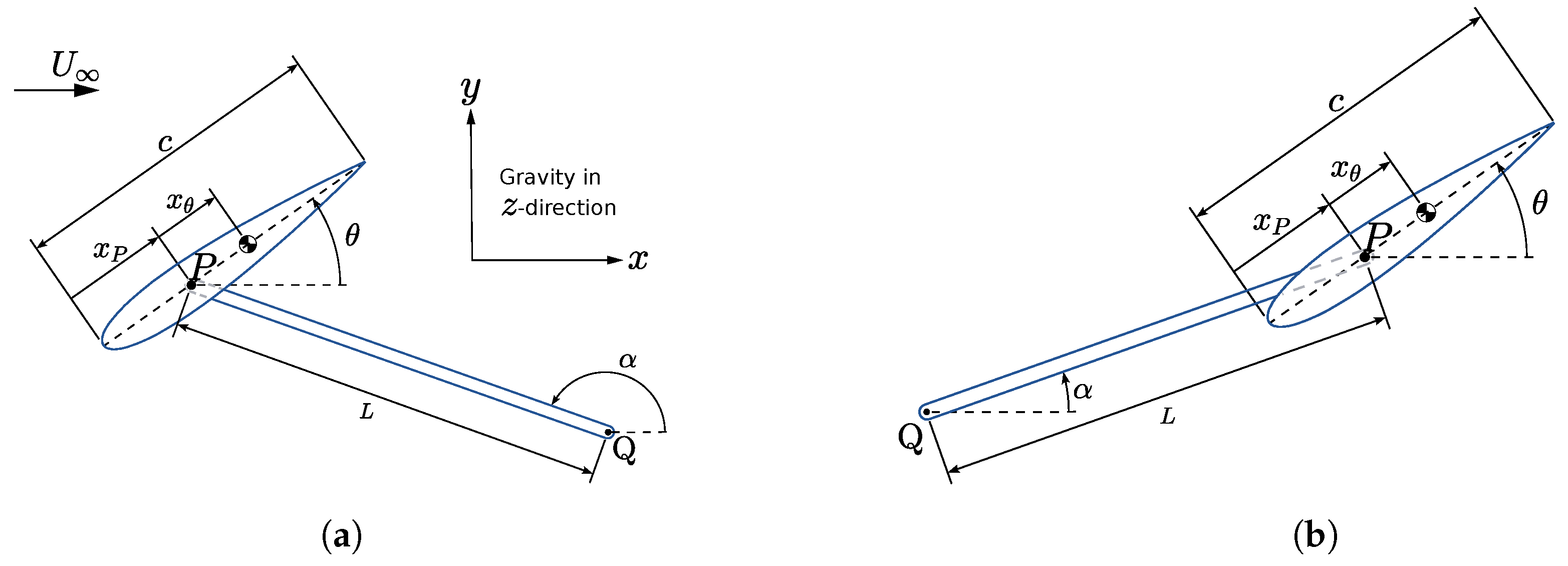
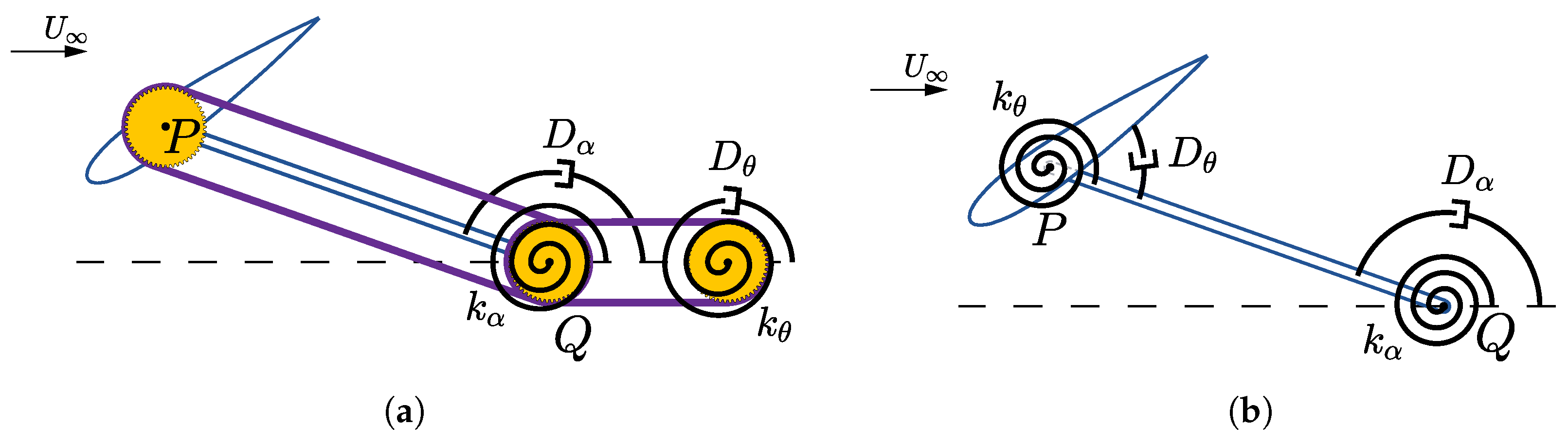
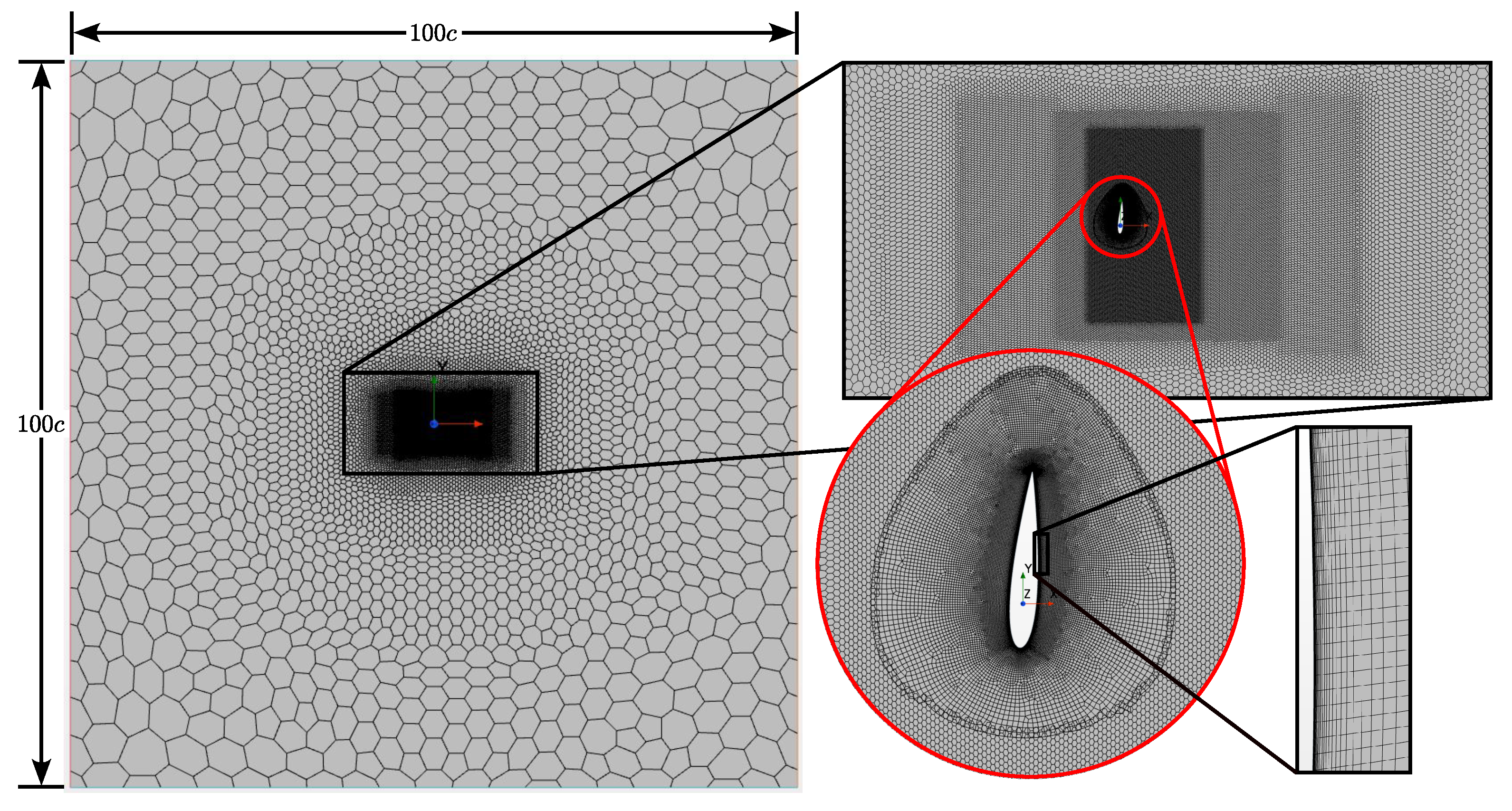
In this study, a new variant of the FP-OFT is investigated, where the foil is placed upon a swinging arm rather than on rails. This FP-OFT on a swinging arm (FP-OFT-SA) thus has the advantage of being mechanically much simpler. Indeed, a single pivot offers fewer mechanical constraints than rails, which have to be perfectly aligned to ensure proper sliding of the foil in the heaving motion. However, the effects of the foil’s circular trajectory are not well documented for the FP-OFT, thus motivating this research. Upstream and downstream rest positions are investigated with two variants regarding the setup for the pitch spring and damper. In order to assess the performance of this turbine concept, 2D URANS CFD simulations are carried out to evaluate its efficiency and power coefficient when using structural parameters derived from those of railed configurations from Boudreau et al. [7] and Veilleux and Dumas [18], while operating under, respectively, the coupled-flutter and stall-flutter instabilities. Indeed, the main contribution of this paper is to provide a better understanding of the swinging-arm oscillating-foil turbine and to determine operating configurations that reproduce or even improve the high performances predicted for the railed configurations that undergo a similar but linear motion.

2. Methodology

2.1. Dynamics

To establish parallels with previous results on FP-OFTs using the railed configuration, two chord-based Reynolds numbers were available. For the stall-flutter instability studied by Veilleux and Dumas [18], their optimization was based on a Reynolds number of $5\times {10}^5$, while Boudreau et al. [7] used a Reynolds number of $3.9\times {10}^6$ for their optimization of the coupled-flutter instability. Since a Reynolds number of $5\times {10}^5$ can be considered somewhat low and too close to the transitional regime, and to avoid transition effects in the CFD simulations and the need for a transition model, it was deemed more conservative to use a Reynolds number that would guarantee fully turbulent boundary layers. Secondly, evaluating the two instability modes at the same Reynolds number seemed more appropriate to accurately compare their performances relative to one another under the same flow conditions. For this reason, it was decided to consider only a chord-based Reynolds number of

$${\mathrm{Re}}_c={\displaystyle \frac{U_{\infty }c}{\nu }}=3.9\times {10}^6,$$

(1)

which is reported as being in a Reynolds independent regime for this application [7]. Both instability modes are investigated here using a NACA 0015 foil.

In essence, an FP-OFT-SA is a turbine that is free to move in pitch and to rotate about a circular path, with only springs and dampers passively restricting its movements. However, since the foil can be placed either upstream or downstream of the arm’s pivot point (see Figure 1) and a gear system can be used or not to select the resting angle $\beta$ of the pitch spring between the foil and the flow (see Figure 2 and Figure 3) and to alleviate a resistive torque of the arm, four distinct configurations are analyzed in this paper.

The damper and spring positions are illustrated in Figure 3a,b. In Figure 3a, the pitching spring and damper were moved to a second set of gears and chain to facilitate comprehension, but in practice, they could easily be superimposed on those at point Q without affecting the dynamic equations. As is clearly shown in Figure 3b, the pitching spring and damper are directly mounted on the swinging arm. One can thus observe that the resting position of the foil, for instance, when it is allowed to freely oscillate in a vacuum, is when the foil is parallel to the arm. With the configuration of Figure 3a, however, the pitching spring and damper are now fixed to the horizontal reference, making the resting position of the foil aligned with the horizontal and, therefore, with the flow.

The four configurations are governed by four different pairs of equations of motion which, by defining appropriate dimensionless parameters, are written in a manner that permits a much easier comparison between various cases. The dimensionless parameters used in this study are the same as those used by Boudreau et al. [7] and Veilleux & Dumas [18], with the exception of $L^{*}$ in Equation (2a), which is specific to this study:

$$\begin{array}{c}\hfill L^{*}={\displaystyle \frac{L}{c}},\end{array}$$

(2a)

$$\begin{array}{c}\hfill {\dot{\theta }}^{*}={\displaystyle \frac{\dot{\theta }c}{U_{\infty }}},{\dot{\alpha }}^{*}={\displaystyle \frac{\dot{\alpha }c}{U_{\infty }}},\end{array}$$

(2b)

$$\begin{array}{c}\hfill {\ddot{\theta }}^{*}={\displaystyle \frac{\ddot{\theta }{c}^2}{U_{\infty }^2}},{\ddot{\alpha }}^{*}={\displaystyle \frac{\ddot{\alpha }{c}^2}{U_{\infty }^2}},\end{array}$$

(2c)

$$\begin{array}{c}\hfill k_{\theta }^{*}={\displaystyle \frac{k_{\theta }}{\rho U_{\infty }^{2}b{c}^2}},k_{\alpha }^{*}={\displaystyle \frac{k_{\alpha }}{\rho U_{\infty }^{2}b{c}^2}},\end{array}$$

(2d)

$$\begin{array}{c}\hfill D_{\theta }^{*}={\displaystyle \frac{D_{\theta }}{\rho U_{\infty }b{c}^3}},D_{\alpha }^{*}={\displaystyle \frac{D_{\alpha }}{\rho U_{\infty }b{c}^3}},\end{array}$$

(2e)

$$\begin{array}{c}\hfill I_{\theta }^{*}={\displaystyle \frac{I_{\theta }}{\rho b{c}^4}},I_B^{*}={\displaystyle \frac{I_B}{\rho b{c}^4}},\end{array}$$

(2f)

$$\begin{array}{c}\hfill S^{*}={\displaystyle \frac{S}{\rho b{c}^3}},\end{array}$$

(2g)

$$\begin{array}{c}\hfill C_M={\displaystyle \frac{M}{0.5\rho U_{\infty }^{2}b{c}^2}},\end{array}$$

(2h)

$$\begin{array}{c}\hfill C_{F_y}={\displaystyle \frac{F_y}{0.5\rho U_{\infty }^{2}bc}},C_{F_x}={\displaystyle \frac{F_x}{0.5\rho U_{\infty }^{2}bc}},\end{array}$$

(2i)

where L is the length of the swinging arm, $\theta$ is the pitch angle of the foil, $\alpha$ is the angular position of the arm, $k_{\theta }$ is the stiffness of the foil’s spring at point P, $k_{\alpha }$ is the stiffness of the arm’s spring at point Q, $D_{\theta }$ is the coefficient of the foil’s damper at point P, $D_{\alpha }$ is the coefficient of the arm’s damper at point Q, $I_{\theta }$ is the moment of inertia of the foil measured at point P, $I_B$ is the combination of the mass moment of inertia of the arm measured at point Q and the added mass m of the foil at the end of the arm, i.e., $I_B=I_Q+m{L}^2$, S is the static imbalance taking into consideration the displacement of the foil’s center of mass from point P, i.e., $S=m{x}_{\theta }$, M is the hydrodynamic torque acting on the foil, $F_y$ and $F_x$ are the hydrodynamic forces acting on the foil, $\rho$ is the fluid density, $U_{\infty }$ is the freestream velocity, c is the foil’s chord length, and b is the foil’s span length. For a 2D analysis such as this one, the foil’s span length is considered to be equal to unity $\left(b=1\right)$ for normalization purposes, and hydrodynamic forces on the arm are neglected.

Analyzing the FP-OFT-SA by summing the forces and torques on the foil and the arm produces a pair of equations of motion describing its dynamic response. These pairs of equations link the two degrees of freedom of the system, namely the foil’s pitch angle $\theta$ and the swinging arm’s angular position $\alpha$. Again, for the proposed configurations, four pairs of dimensionless equations are obtained:

• Upstream without gears

$$\begin{array}{c}\hfill {\displaystyle \frac{\left[C_{F_y}cos\left(\alpha \right)-C_{F_x}sin\left(\alpha \right)\right]L^{*}}{2}}=I_B^{*}{\ddot{\alpha }}^{*}+D_{\alpha }^{*}{\dot{\alpha }}^{*}+k_{\alpha }^{*}\left(\alpha -\pi \right)-D_{\theta }^{*}\left({\dot{\theta }}^{*}-{\dot{\alpha }}^{*}\right)\\ \hfill -k_{\theta }^{*}\left(\theta +\pi -\alpha \right)+S^{*}{L}^{*}\left[{\ddot{\theta }}^{*}cos\left(\theta -\alpha \right)-{{\dot{\theta }}^{*}}^{2}sin\left(\theta -\alpha \right)\right],\end{array}$$

(3a)

$$\begin{array}{c}\hfill {\displaystyle \frac{C_M}{2}}=I_{\theta }^{*}{\ddot{\theta }}^{*}+D_{\theta }^{*}({\dot{\theta }}^{*}-{\dot{\alpha }}^{*})+k_{\theta }^{*}(\theta +\pi -\alpha )+S^{*}{L}^{*}\left[{\ddot{\alpha }}^{*}cos(\theta -\alpha )+{{\dot{\alpha }}^{*}}^{2}sin(\theta -\alpha )\right],\end{array}$$

(3b)

• Upstream with gears

$$\begin{array}{c}\hfill {\displaystyle \frac{\left[C_{F_y}cos\left(\alpha \right)-C_{F_x}sin\left(\alpha \right)\right]L^{*}}{2}}=I_B^{*}{\ddot{\alpha }}^{*}+D_{\alpha }^{*}{\dot{\alpha }}^{*}+k_{\alpha }^{*}(\alpha -\pi )\\ \hfill +S^{*}{L}^{*}\left[{\ddot{\theta }}^{*}cos(\theta -\alpha )-{{\dot{\theta }}^{*}}^{2}sin(\theta -\alpha )\right],\end{array}$$

(4a)

$$\begin{array}{c}\hfill {\displaystyle \frac{C_M}{2}}=I_{\theta }^{*}{\ddot{\theta }}^{*}+D_{\theta }^{*}{\dot{\theta }}^{*}+k_{\theta }^{*}\theta +S^{*}{L}^{*}\left[{\ddot{\alpha }}^{*}cos(\theta -\alpha )+{{\dot{\alpha }}^{*}}^{2}sin(\theta -\alpha )\right],\end{array}$$

(4b)

• Downstream without gears

$$\begin{array}{c}\hfill {\displaystyle \frac{\left[C_{F_y}cos\left(\alpha \right)-C_{F_x}sin\left(\alpha \right)\right]L^{*}}{2}}=I_B^{*}{\ddot{\alpha }}^{*}+D_{\alpha }^{*}{\dot{\alpha }}^{*}+k_{\alpha }^{*}\alpha -D_{\theta }^{*}({\dot{\theta }}^{*}-{\dot{\alpha }}^{*})-k_{\theta }^{*}(\theta -\alpha )\\ \hfill +S^{*}{L}^{*}\left[{\ddot{\theta }}^{*}cos(\theta -\alpha )-{{\dot{\theta }}^{*}}^{2}sin(\theta -\alpha )\right],\end{array}$$

(5a)

$$\begin{array}{c}\hfill {\displaystyle \frac{C_M}{2}}=I_{\theta }^{*}{\ddot{\theta }}^{*}+D_{\theta }^{*}({\dot{\theta }}^{*}-{\dot{\alpha }}^{*})+k_{\theta }^{*}(\theta -\alpha )+S^{*}{L}^{*}\left[{\ddot{\alpha }}^{*}cos(\theta -\alpha )+{{\dot{\alpha }}^{*}}^{2}sin(\theta -\alpha )\right],\end{array}$$

(5b)

• Downstream with gears

$$\begin{array}{c}\hfill {\displaystyle \frac{\left[C_{F_y}cos\left(\alpha \right)-C_{F_x}sin\left(\alpha \right)\right]L^{*}}{2}}=I_B^{*}{\ddot{\alpha }}^{*}+D_{\alpha }^{*}{\dot{\alpha }}^{*}+k_{\alpha }^{*}\alpha \\ \hfill +S^{*}{L}^{*}\left[{\ddot{\theta }}^{*}cos(\theta -\alpha )-{{\dot{\theta }}^{*}}^{2}sin(\theta -\alpha )\right],\end{array}$$

(6a)

$$\begin{array}{c}\hfill {\displaystyle \frac{C_M}{2}}=I_{\theta }^{*}{\ddot{\theta }}^{*}+D_{\theta }^{*}{\dot{\theta }}^{*}+k_{\theta }^{*}\theta +S^{*}{L}^{*}\left[{\ddot{\alpha }}^{*}cos(\theta -\alpha )+{{\dot{\alpha }}^{*}}^{2}sin(\theta -\alpha )\right].\end{array}$$

(6b)

When the system is gearless, the pitch spring is directly mounted upon the foil and the arm. In such a case, the equilibrium position $\beta$ of the foil is where the foil is parallel to the arm, i.e., $\beta =\alpha$, as is shown in Figure 2a. In any other angular position, a torque is then applied by the pitch spring on the foil. From Newton’s third law, an equal and opposite torque is therefore applied on the arm. This can be seen in Equations (3a) and (5a) where the terms involving the pitch damper $D_{\theta }^{*}$ and pitch spring $k_{\theta }^{*}$ are present when the system is gearless, but are absent in Equations (4a) and (6a) when the system is geared.

In the gearless configurations, these additional terms are always present, but they become increasingly negligible as the length of the arm increases. Indeed, as will be shown in Section 2.2, the equations of motion, for both the geared and the gearless configurations, tend back to the railed configuration’s equations of motion the longer the arm.

As will be discussed in Section 3, this detail pertaining to these additional terms, which might seem minor at the moment, will lead to major differences in performances of the turbine.

2.2. Extrapolating the Structural Parameters from the Optimized Railed Cases

From any pair of dynamic equations presented in Section 2.1, it is obvious that optimizing the behavior of such a system represents quite a task because of the numerous parameters. However, the dynamic equations of the FP-OFT-SA share much similarity with those of the railed FP-OFT, for which sets of structural parameters have already been optimized and are readily available from previous studies [7,18]. The following Equations (7a) and (7b) are the equations of motion in heave and in pitch for the railed FP-OFT, where h represents the heaving displacement of the foil:

• On rails

$$\begin{array}{c}\hfill {\displaystyle \frac{C_{F_y}}{2}}=m_h^{*}{\ddot{h}}^{*}+D_h^{*}{\dot{h}}^{*}+k_h^{*}{h}^{*}+S^{*}\left[{\ddot{\theta }}^{*}cos\left(\theta \right)-{{\dot{\theta }}^{*}}^{2}sin\left(\theta \right)\right],\end{array}$$

(7a)

$$\begin{array}{c}\hfill {\displaystyle \frac{C_M}{2}}=I_{\theta }^{*}{\ddot{\theta }}^{*}+D_{\theta }^{*}{\dot{\theta }}^{*}+k_{\theta }^{*}\theta +S^{*}{\ddot{h}}^{*}cos\left(\theta \right).\end{array}$$

(7b)

A strong resemblance is observed between the pair of Equations (7a) and (7b) and the four pairs of Equations (3a)–(6b). We thus propose, in order to assess the performance of the FP-OFT-SA, to establish its parameters based on those of the railed configuration. In fact, for a given heaving amplitude $H_0$ of the FP-OFT-SA, when the ratio of the swinging arm length to this heave amplitude tends towards infinity, i.e., ${\displaystyle \frac{L}{H_0}}\to \infty$, the motion of point P tends towards a completely linear heaving motion, i.e., the motion of the railed configuration. Inversely, when the ratio of the swinging arm length to the heave amplitude is small, for instance when ${\displaystyle \frac{L}{H_0}}=\mathcal{O}\left(1\right)$, then the motion of point P traces a clearly visible arc, as is shown in Figure 4b,c. This can be demonstrated with any of the four pairs of dynamic equations presented in Section 2.1. For instance, using the downstream configuration, which oscillates about the $\alpha =0$ reference, $sin\left(\alpha \right)\simeq 0$ and $cos\left(\alpha \right)\simeq 1$ when ${\displaystyle \frac{L}{H_0}}\to \infty$ because $\alpha \simeq 0$ throughout the cycle. Furthermore, as stated previously, the displacement of point P becomes essentially linear and $h^{*}\simeq L^{*}\alpha$, which means that $\dot{h^{*}}\simeq L^{*}\dot{\alpha }$ and $\ddot{h^{*}}\simeq L^{*}\ddot{\alpha }$. After substitutions and simplifications, Equations (3a)–(6b) become:

$$\begin{array}{c}\hfill {\displaystyle \frac{C_{F_y}}{2}}={\displaystyle \frac{I_B^{*}{\ddot{h}}^{*}}{{L^{*}}^2}}+{\displaystyle \frac{D_{\alpha }^{*}{\dot{h}}^{*}}{{L^{*}}^2}}+{\displaystyle \frac{k_{\alpha }^{*}{h}^{*}}{{L^{*}}^2}}+S^{*}\left[{\ddot{\theta }}^{*}cos\left(\theta \right)-{{\dot{\theta }}^{*}}^{2}sin\left(\theta \right)\right],\end{array}$$

(8a)

$$\begin{array}{c}\hfill {\displaystyle \frac{C_M}{2}}=I_{\theta }^{*}{\ddot{\theta }}^{*}+D_{\theta }^{*}{\dot{\theta }}^{*}+k_{\theta }^{*}\theta +S^{*}{\ddot{h}}^{*}cos\left(\theta \right).\end{array}$$

(8b)

Equations (8a) and (8b) now have the same form as Equations (7a) and (7b). Therefore, knowing the dimensionless parameters of a railed FP-OFT, equivalent parameters for the FP-OFT-SA can easily be derived:

$$\begin{array}{c}\hfill I_B^{*}=m_h^{*}{L^{*}}^2,\end{array}$$

(9a)

$$\begin{array}{c}\hfill D_{\alpha }^{*}=D_h^{*}{L^{*}}^2,\end{array}$$

(9b)

$$\begin{array}{c}\hfill k_{\alpha }^{*}=k_h^{*}{L^{*}}^2.\end{array}$$

(9c)

As for $S^{*}$, $I_{\theta }^{*}$, $D_{\theta }^{*}$, and $k_{\theta }^{*}$, their values do not depend upon $L^{*}$, and they are therefore kept identical to those of the optimized railed configurations.

When $L^{*}$ is small, there is no guarantee that the swinging model will behave similarly to the railed model because of the aforementioned arched motion of point P. To test the FP-OFT-SA, two sets of optimized structural parameters of the railed FP-OFT, each involving a different type of flow instability, have been selected from previous publications. From the work of Boudreau et al. [7] on FP-OFTs operating under the coupled-flutter instability, a set of parameters achieving the best efficiency of 51.0% was selected, while from Veilleux and Dumas’s work [18] on FP-OFTs operating under the stall-flutter instability, their most optimized case, reaching an efficiency of 33.6%, was selected.

Table 1. Structural parameters of the optimized coupled-flutter and stall-flutter railed FP-OFT configurations.

Parameter	Coupled-Flutter (Boudreau et al. [7])	Stall-Flutter (Veilleux and Dumas [18])
$x_P/c$	$1/4$	$1/3$
$m_h^{*}$	2	3.036
$D_h^{*}$	0.7	1.501
$k_h^{*}$	1.55	1.206
$I_{\theta }^{*}$	2	0.095
$D_{\theta }^{*}$	0	0.119
$k_{\theta }^{*}$	3.16	0.031
$S^{*}$	0.65	−0.029

shows the values of the different parameters leading to the two instabilities analyzed, from which Equations (9a)–(9c) are used to find the structural parameters of the swinging arm configuration as a function of $L^{*}$. We emphasize again that for stall-flutter instability, the pitch axis is placed downstream of the center of pressure $x_P/c=1/3$ in order for the divergence instability to occur.

2.3. Performance Metrics

The power extracted from the flow by the FP-OFT-SA has three components, stemming from the two force components $F_x$ and $F_y$ and the pitch torque M experienced by the foil. Using the dimensionless parameters presented in Section 2.1, the following mean power coefficients are defined:

$$\begin{array}{c}\hfill \langle C_{P_y}\rangle ={\displaystyle \frac{1}{T^{*}}}{\int }_{t_i^{*}}^{t_i^{*}+T^{*}}{C}_{F_y}{L}^{*}cos\left(\alpha \right){\dot{\alpha }}^{*}d{t}^{*},\end{array}$$

(10)

$$\begin{array}{c}\hfill \langle C_{P_x}\rangle ={\displaystyle \frac{-1}{T^{*}}}{\int }_{t_i^{*}}^{t_i^{*}+T^{*}}{C}_{F_x}{L}^{*}sin\left(\alpha \right){\dot{\alpha }}^{*}d{t}^{*},\end{array}$$

(11)

$$\begin{array}{c}\hfill \langle C_{P_{\theta }}\rangle ={\displaystyle \frac{1}{T^{*}}}{\int }_{t_i^{*}}^{t_i^{*}+T^{*}}{C}_M{\dot{\theta }}^{*}d{t}^{*},\end{array}$$

(12)

and the global power coefficient of the turbine is given by:

$$\begin{array}{c}\hfill \langle C_P\rangle =\langle C_{P_y}\rangle +\langle C_{P_x}\rangle +\langle C_{P_{\theta }}\rangle ,\end{array}$$

(13)

where the angle brackets signify cycle-averaged values, $t_i^{*}$ is the initial dimensionless time $\left(t^{*}=t{U}_{\infty }/c\right)$ of a given cycle, and $T^{*}$ is the dimensionless period of a cycle. Note that, for the rest of the study, the term power coefficient refers to these cycle-averaged values unless stated otherwise.

Another important performance metric is the energy extraction efficiency $\eta$, defined as the ratio of the cycle-averaged power extracted by the turbine $\langle P\rangle$ to the power available in the incoming flow passing through the swept area of the foil:

$$\eta ={\displaystyle \frac{\langle P\rangle }{1/2\rho U_{\infty }^{3}bd}},$$

(14)

where d is the overall height of the power extraction window calculated from the highest and lowest points reached by any part of the foil during a cycle from the combined effect of both the heave and pitch amplitudes (see Figure 5).

2.4. Numerics

2.4.1. Fluid-Structure Interaction Algorithm

The simulations in this study have been carried out with an in-house implicit fluid-structure interaction (FSI) algorithm implemented in Siemens STAR-CCM+^®, version 2021.2, build 16.04.007-R8 [25], to calculate the displacement of an overset mesh containing the NACA 0015 foil. The fluid solver is based on the unsteady incompressible Reynolds Averaged Navier-Stokes (URANS) equations, and it uses the Spalart-Allmaras one-equation turbulence model since the Reynolds number is high enough to assume fully turbulent boundary layers. The pressure-velocity coupling is handled with the SIMPLE algorithm [26,27], and the discretization is based on a second-order finite-volume method.

The FSI algorithm follows a coupling scheme developed by Olivier and Paré-Lambert [28], which was shown to be a stable method for strong coupling FSI. The solver works by approximating the foil’s position from the last known forces and torques, moving the foil according to the approximated displacement calculated from the discretized versions of the equations of motion presented in Section 2.1. These equations are discretized using a second-order backward difference scheme, and the FSI algorithm then solves the system of linear equations using Broyden’s method [29], for which the solid criteria are based upon controlling the normalized dynamic residual of both swinging and pitching equations, recalculating the fluid behavior from this estimated displacement, and then repositioning the foil accordingly in an iterative process until both the fluid and solid convergence criteria are reached.

2.4.2. Iterative Convergence Criteria

Once the normalized residuals of the swinging and pitching equations are less than ${10}^{-5}$, the solid solver is considered converged. For the fluid solver, convergence is considered to be achieved when the relative variation of forces $F_x$, $F_y$, and the torque M, between two outer steps occurring during the looping of a unique time step, is smaller than ${10}^{-7}$. The momentum residual in both X and Y, as well as the continuity residual, must be smaller than ${10}^{-4}$ while the residual of the turbulent viscosity equation in the Spalart–Allmaras model must fall under $5\times {10}^{-4}$. These values offered performance metrics in good agreement with those reported by Boudreau et al. [7], as is shown in

Table 2. Comparison between the current study railed performance metrics and the optimized case performance metrics reported by Boudreau et al. [7].

Parameter	Boudreau et al. [7]	Current Study	Rel. Diff.
$\overline{H_0^{*}}$	1.14	1.13	−0.9%
$\overline{{\mathsf{\Theta }}_0^{*}}$	70°–95°	91.1°	-
$\overline{\varphi }$	95°–110°	96.6°	-
$\overline{\eta }$	51.0%	50.6%	−0.8%
$\overline{C_P}$	1.41	1.39	−1.4%
$\overline{C_x}$	3.69	3.63	−1.6%
${\sigma }_{\eta }$	0.015	0.031	-

.

2.4.3. CFD Domain and Mesh

In this study, the background mesh forms a square with side lengths of 100 cords containing 49,291 hexagonal cells (see Figure 6). In the center of this square are zones of progressively increasing refinement. An overset mesh containing a NACA 0015 foil is placed in the most refined zone. The overset mesh is made of 29,323 cells and has 500 nodes placed around its periphery. It was verified that the $y+$ value is everywhere close to unity during a statistically converged cycle. Both meshes are combined using an overset mesh feature integrated in STAR-CCM+^®. At the inlet (left border), a uniform velocity profile along with a uniform turbulent viscosity ratio $\tilde{\nu }/\nu =3$ is applied. This viscosity ratio follows the recommendation by [30] to ensure that the Sparlart-Allmaras turbulence model operates in its fully turbulent mode. Additionally, a zero-gauge pressure is applied on the outlet (right border), and symmetric conditions are applied on the upper and bottom borders of the domain. For all simulations, the time step used is such that $U_{\infty }\Delta t/c=0.005$. This represents at least 1000 time steps per cycle for all simulations carried out. Table 2 shows the main performance metrics obtained in the current study for the railed configuration operating under the coupled-flutter instability and their values obtained by Boudreau et al. [7], showing very good agreement between the two and giving a high degree of confidence that the swinging arm results obtained in this study are trustworthy. An experimental study has also been carried out by Boudreau et al. [19] to validate the numerical simulations of Veilleux and Dumas [18], showing good agreement between the numerical and experimental results.

3. Results and Discussion

3.1. Choice of Arm Lengths

As stated in Section 2.1, the longer the arm, the more the foil’s motion will become similar to that of the railed FP-OFT. Inversely, shorter arms will make the foil trace an arched trajectory. Thus, to cover small to moderately long lengths of the arm (normalized with the chord of the foil), the following values were chosen: $1, 2, 3, 4, 5, 6, 7.5, 10, 100$, and 1000. The last two very large lengths, i.e., 100 and 1000, which are obviously impractical choices for building prototypes, were chosen to validate the fact that as ${\displaystyle \frac{L^{*}}{H_0^{*}}}\to \infty$, the performances of all configurations tend to those of the railed FP-OFT. This can be observed in Figure 7, where the instantaneous power coefficient $C_P$ of the FP-OFT-SA is shown during a complete cycle as a function of the dimensionless length of the arm operating under the coupled-flutter and the stall-flutter instabilities.

As $L^{*}$ increases, the curves fall back to the railed FP-OFT curve. This can be observed in Figure 8 and Figure 9, which show the normalized vorticity field of half a cycle of the cases shown in Figure 7, as well as the arched trajectory with smaller values of $L^{*}$. The vorticity fields also show the different vortex shedding patterns between the coupled-flutter and the stall-flutter parameters. Note that, in some instances, additional arm lengths in the small-to-moderate range have been analyzed in order to add resolution in some regions of the performance metrics’ curves.

Table 3. Performance metrics for the FP-OFT-SA using the upstream geared configuration and operating under both the coupled-flutter and the stall-flutter instabilities. Standard deviations (SD) are also presented, as defined at the end of Section 3.1.

	Coupled-Flutter				Stall-Flutter
$L^{*}$	$C_P$ (SD)	$\eta$% (SD)	$T^{*}$ (SD)	$d^{*}$ (SD)	$C_P$ (SD)	$\eta$% (SD)	$T^{*}$ (SD)	$d^{*}$ (SD)
1	0.52 (0.00)	27.3 (0.0)	5.09 (0.00)	1.90 (0.00)	0.41 (0.04)	16.7 (1.4)	23.89 (6.76)	2.43 (0.11)
2	1.43 (0.00)	51.9 (0.0)	5.11 (0.00)	2.76 (0.00)	0.48 (0.08)	15.9 (2.2)	17.65 (2.46)	3.02 (0.11)
3	1.50 (0.04)	53.6 (1.2)	5.05 (0.01)	2.80 (0.02)	0.77 (0.05)	23.0 (1.2)	13.91 (0.30)	3.36 (0.06)
4	1.44 (0.05)	52.2 (1.3)	5.01 (0.01)	2.76 (0.03)	0.84 (0.00)	24.0 (0.0)	13.42 (0.00)	3.49 (0.00)
5	1.57 (0.06)	54.7 (1.5)	5.00 (0.01)	2.86 (0.03)	0.90 (0.00)	25.3 (0.0)	13.06 (0.00)	3.55 (0.00)
6	1.52 (0.02)	54.1 (0.0)	5.00 (0.01)	2.81 (0.04)	0.93 (0.00)	26.2 (0.0)	12.81 (0.00)	3.57 (0.00)
7.5	1.48 (0.10)	53.2 (2.5)	4.98 (0.01)	2.79 (0.07)	0.98 (0.00)	27.4 (0.0)	12.49 (0.00)	3.59 (0.00)
10	1.48 (0.08)	52.9 (2.1)	4.97 (0.02)	2.81 (0.05)	1.07 (0.11)	30.2 (2.9)	11.91 (0.52)	3.56 (0.04)
100	1.44 (0.13)	52.0 (3.4)	4.94 (0.02)	2.77 (0.09)	1.06 (0.07)	32.1 (2.2)	11.15 (0.40)	3.30 (0.03)
1000	1.34 (0.12)	50.3 (3.1)	4.93 (0.01)	2.67 (0.08)	1.03 (0.01)	30.6 (0.0)	11.77 (0.05)	3.35 (0.03)

,

Table 4. Performance metrics for the FP-OFT-SA using the upstream gearless configuration and operating under both the coupled-flutter and the stall-flutter instabilities. Standard deviations (SD) are also presented, as defined at the end of Section 3.1.

	Coupled-Flutter				Stall-Flutter
$L^{*}$	$C_P$ (SD)	$\eta$% (SD)	$T^{*}$ (SD)	$d^{*}$ (SD)	$C_P$ (SD)	$\eta$% (SD)	$T^{*}$ (SD)	$d^{*}$ (SD)
1	0.03 (0.00)	1.5 (0.0)	29.28 (0.00)	2.03 (0.00)	0.21 (0.03)	9.9 (1.0)	33.09 (30.02)	2.14 (0.55)
2	−0.05 (0.06)	−6.7 (5.7)	5.02 (0.18)	0.61 (0.28)	0.53 (0.05)	16.0 (1.3)	26.60 (3.90)	3.33 (0.17)
3	0.00 (0.00)	0.0 (0.0)	5.05 (0.01)	0.16 (0.00)	0.58 (0.07)	18.9 (4.5)	16.12 (2.45)	3.15 (0.45)
4	0.00 (0.00)	0.0 (0.0)	5.03 (0.00)	0.16 (0.00)	0.69 (0.00)	20.4 (0.0)	14.05 (0.00)	3.40 (0.00)
5	0.00 (0.00)	0.0 (0.0)	5.02 (0.00)	0.17 (0.00)	0.76 (0.00)	22.0 (0.0)	13.56 (0.00)	3.47 (0.00)
6	0.00 (0.00)	0.0 (0.0)	5.00 (0.00)	0.16 (0.00)	0.82 (0.00)	23.5 (0.0)	13.17 (0.00)	3.51 (0.00)
7.5	0.07 (0.00)	8.9 (0.0)	4.99 (0.00)	0.75 (0.00)	0.89 (0.00)	25.2 (0.0)	12.74 (0.01)	3.54 (0.00)
10	0.34 (0.00)	22.5 (0.0)	4.99 (0.00)	1.53 (0.00)	0.97 (0.00)	27.5 (0.0)	12.22 (0.00)	3.55 (0.00)
100	1.34 (0.01)	49.1 (0.0)	4.94 (0.00)	2.73 (0.03)	1.03 (0.09)	31.0 (2.6)	11.36 (0.44)	3.32 (0.03)
1000	1.39 (0.10)	51.0 (2.5)	4.94 (0.01)	2.74 (0.07)	1.16 (0.12)	34.1 (2.8)	10.89 (0.53)	3.40 (0.10)

,

Table 5. Performance metrics for the FP-OFT-SA using the downstream geared configuration and operating under both the coupled-flutter and the stall-flutter instabilities. Standard deviations (SD) are also presented, as defined at the end of Section 3.1.

	Coupled-Flutter				Stall-Flutter
$L^{*}$	$C_P$ (SD)	$\eta$% (SD)	$T^{*}$ (SD)	$d^{*}$ (SD)	$C_P$ (SD)	$\eta$% (SD)	$T^{*}$ (SD)	$d^{*}$ (SD)
1	0.46 (0.05)	26.5 (1.7)	4.86 (0.05)	1.72 (0.07)	0.40 (0.00)	19.7 (0.0)	10.46 (0.00)	2.04 (0.00)
2	1.08 (0.03)	43.4 (1.1)	4.83 (0.00)	2.49 (0.02)	0.61 (0.00)	24.9 (0.0)	10.63 (0.00)	2.46 (0.00)
3	1.21 (0.09)	46.4 (2.8)	4.86 (0.01)	2.60 (0.06)	0.80 (0.00)	30.4 (0.0)	10.08 (0.00)	2.62 (0.00)
4	1.21 (0.05)	46.6 (1.4)	4.88 (0.01)	2.61 (0.03)	0.87 (0.00)	31.8 (0.0)	10.12 (0.00)	2.73 (0.00)
5	1.31 (0.06)	48.7 (1.6)	4.89 (0.01)	2.68 (0.04)	0.92 (0.00)	32.7 (0.0)	10.16 (0.00)	2.80 (0.00)
6	1.31 (0.12)	48.7 (3.2)	4.89 (0.01)	2.69 (0.07)	0.95 (0.00)	33.2 (0.0)	10.18 (0.00)	2.86 (0.00)
7.5	1.28 (0.11)	47.9 (3.1)	4.90 (0.01)	2.66 (0.07)	0.95 (0.06)	32.2 (2.2)	10.50 (0.37)	2.95 (0.02)
10	1.34 (0.13)	49.9 (3.6)	4.91 (0.01)	2.68 (0.08)	0.94 (0.09)	30.6 (2.9)	10.94 (0.41)	3.06 (0.03)
100	1.44 (0.09)	51.8 (2.3)	4.94 (0.02)	2.78 (0.06)	1.05 (0.08)	32.4 (2.6)	10.98 (0.48)	3.23 (0.04)
1000	1.41 (0.14)	51.0 (3.7)	4.94 (0.02)	2.76 (0.09)	1.04 (0.08)	31.6 (2.5)	11.18 (0.45)	3.27 (0.04)

and

Table 6. Performance metrics for the FP-OFT-SA using the downstream gearless configuration and operating under both the coupled-flutter and the stall-flutter instabilities. Standard deviations (SD) are also presented, as defined at the end of Section 3.1.

	Coupled-Flutter				Stall-Flutter
$L^{*}$	$C_P$ (SD)	$\eta$% (SD)	$T^{*}$ (SD)	$d^{*}$ (SD)	$C_P$ (SD)	$\eta$% (SD)	$T^{*}$ (SD)	$d^{*}$ (SD)
1	0.00 (0.00)	0.0 (0.0)	2.96 (0.11)	0.15 (0.00)	0.46 (0.02)	22.7 (1.0)	11.29 (0.26)	2.01 (0.00)
2	0.00 (0.00)	0.0 (0.0)	3.83 (0.12)	0.15 (0.00)	0.72 (0.03)	28.1 (1.0)	10.70 (0.26)	2.56 (0.04)
3	0.00 (0.00)	0.0 (0.0)	4.41 (0.00)	0.17 (0.00)	0.80 (0.08)	28.9 (2.2)	10.85 (0.59)	2.77 (0.08)
4	0.00 (0.00)	0.0 (0.0)	4.54 (0.00)	0.15 (0.00)	0.82 (0.00)	28.8 (0.0)	11.21 (0.00)	2.84 (0.00)
5	0.11 (0.00)	11.8 (0.0)	4.69 (0.01)	0.93 (0.00)	0.95 (0.06)	32.3 (1.5)	10.52 (0.51)	2.95 (0.06)
6	0.13 (0.05)	12.6 (4.9)	4.79 (0.05)	0.99 (0.00)	0.91 (0.00)	30.0 (0.0)	11.24 (0.01)	3.02 (0.01)
7.5	0.15 (0.03)	13.1 (2.2)	4.87 (0.07)	1.13 (0.02)	0.95 (0.05)	31.4 (1.7)	10.93 (0.33)	3.02 (0.04)
10	0.18 (0.17)	12.7 (10.9)	4.99 (0.09)	1.31 (0.19)	0.95 (0.07)	30.9 (2.2)	11.03 (0.46)	3.09 (0.05)
100	1.41 (0.10)	51.3 (2.5)	4.93 (0.01)	2.75 (0.06)	1.01 (0.06)	30.8 (2.0)	11.31 (0.30)	3.27 (0.03)
1000	1.44 (0.14)	51.4 (3.6)	4.94 (0.02)	2.79 (0.09)	1.05 (0.07)	32.2 (2.2)	11.08 (0.43)	3.27 (0.05)

show the values of the efficiency, the power coefficient, the period, and the extraction window of the FP-OFT-SA as a function of the dimensionless length of the arm operating under the coupled-flutter instability and the stall-flutter instability, respectively. These values are also presented in Figure 10a,b, Figure 11a,b, Figure 12a,b and Figure 13a,b. The red region in Figure 10 and Figure 11 represents the negative values of the efficiency or the power coefficient, meaning that the power is transferred from the foil to the flow, while the error bars in all figures, as well as the grey regions, represent the standard deviation (SD) from the mean of the last ten cycles when the relative difference in efficiency of the last two cycles was not less than or equal to $0.1\%$.

3.2. Coupled-Flutter Instability

3.2.1. Geared

Figure 11a shows that, operating under the coupled-flutter instability, the two most efficient configurations are those using gears. In these configurations, the values of the efficiency follow similar trends, with the upstream and downstream configurations being respectively superior and inferior to the railed baseline for $L^{*}\ge 2$. This difference in performances, which has been observed previously by Jiang et al. [31] and Sitorus and Ko [23], comes from the fact that, in the upstream configuration, the horizontal component of the force (i.e., the drag force) acting on the foil has the effect of pushing the foil against the resistive torque of the arm’s spring. The arm can thus reach higher angular amplitudes, meaning that the extraction window is therefore greater in the upstream configuration, as is confirmed by Figure 13a. From an increase of the extraction window comes a decrease in efficiency if the power is the same (see Equation (14)). However, the power extracted is higher, induced by the vertical component of the force (i.e., the lift force) in the added distance covered in the upstream position. Inversely, in the downstream configuration, the drag force works in conjunction with the arm’s spring, contributing to the deceleration of the arm and, a fortiori, to the reduction of its angular amplitude. The extraction window is therefore diminished, and so is the work done by the vertical component of the force. To illustrate this discussion, Figure 14a shows a comparison between the upstream and downstream configurations of the coupled-flutter turbine with $L^{*}=5$, where one can see the much greater contribution from the vertical force component in the upstream configuration when compared to the downstream configuration.

Interestingly, in the geared configurations, Figure 12a shows that, for the moderate lengths, the period of oscillations tends to diverge slightly more or less symmetrically with respect to the asymptotic railed value. Indeed, in the upstream configuration, the period tends to increase with a decrease of $L^{*}$, while the period in the downstream configuration tends to decrease. However, these diverging values stay within 4% of the railed value.

It is important to also note that in a 3D scenario of the FP-OFT-SA in the downstream configuration, the arm’s wake could possibly significantly hinder the performances, making it even worse than it already is compared to the performances of the upstream configuration.

It is thus clear that the upstream configuration should always be considered as the first option for building prototypes of an FP-OFT-SA operating under the coupled-flutter instability.

3.2.2. Gearless

Still using the coupled-flutter configuration, Figure 11a shows that, when gearless, the system is unresponsive at small to moderate lengths of the arm, i.e., $1\lesssim L^{*}\lesssim 5$, for both upstream and downstream configurations. Indeed, the system, given an initial arm angular velocity and a foil angular position, has decaying amplitudes over time, leading to a complete rest of the turbine given enough cycles.

At larger $L^{*}$, the system in the upstream configuration starts to oscillate in a steady-state regime, with the efficiency increasing with the value of $L^{*}$. As for the system in the downstream configuration, it starts to oscillate erratically, as indicated by the large error bars in Figure 11a. In this range of lengths, the pitch spring’s torque at the pitch axis, which is acting on the arm, is starting to become small enough to let the turbine oscillate, but it remains large enough to momentarily hinder the motion of the arm at various instants in a cycle. Indeed, recall from Equations (3a) and (5a) that the gearless configurations have additional terms involving the pitching structural parameters ($k_{\theta }$ and $D_{\theta }$) in the arm’s equation of motion. As $L^{*}$ increases, these terms vary with ${\left(L^{*}\right)}^{-2}$. Therefore, for low values of $L^{*}$, the pitching terms have a strong relative effect on the dynamic response of the arm. Conversely, as $L^{*}$ increases, these pitching terms become increasingly negligible, which reduces the reaction of the pitch spring’s torque on the arm.

For the period of oscillation in the gearless configurations, Figure 12a shows that it acts similarly to the geared configurations, wherein the period seems to diverge from the asymptotic railed value, with the upstream/downstream configurations having higher/lower periods of oscillation, respectively. However, unlike the geared configurations, the values become very large with large error bars, showing very erratic behavior of the turbines at small length values. This suggests the idea that FP-OFT-SAs using small lengths of the arm and the parameters that led to the coupled-flutter instability of the railed case [7] are not viable configurations and should be discarded for building prototypes. Viable configurations are rather associated with moderate to large lengths of the arm, i.e., $5\lesssim L^{*}\lesssim 10$.

3.3. Stall-Flutter Instability

For the stall-flutter instability, the use of gears is not mandatory to reach steady-state oscillations for any length of the arm. In fact, positive efficiency values are obtained for all lengths, increasing from their lowest values (10–22%) at the smallest length of $L^{*}=1$ to an asymptotic value between 30% and 35% as $L^{*}$ increases (see Figure 11b). Regardless of the length of the arm and the presence or absence of the gear system, the stall-flutter driving mechanism is more robust, although not as efficient, than the coupled-flutter mechanism, which requires gears to operate properly with short arms. In fact, the stall-flutter mechanism rests on a divergence instability of the foil, which brings the foil into a steady-state regime very quickly after its start-up (1 or 2 cycles), using the strong aerodynamic torque at point P during the heaving motion to strongly counteract the pitch spring’s torque. It is only when the suction side boundary layer detaches and an LEV is shed that, suddenly, the aerodynamic torque falls, leading to the pitch spring torque being able to rotate the foil back. It is therefore deduced that, even if the pitch spring is directly attached to the arm in the gearless configuration, the resulting torque applied to the arm is small enough in comparison with the aerodynamic torque, and the turbine can thus continue to operate.

Moreover, as opposed to the coupled-flutter turbine, Figure 11b shows that the most efficient configurations operating under the stall-flutter instability are not related to the use of gears. Indeed, the two best configurations are the downstream configurations, with and without the use of gears. Here, the same argument as in the coupled-flutter instability configuration holds true: the horizontal component of the force tends to increase the extraction window in the upstream configuration and to reduce it in the downstream configuration. However, the upstream coupled-flutter turbine had a higher $C_P$ than its downstream counterpart because of the added power in the heave motion from the larger window. For the stall-flutter case, Figure 10b shows that the $C_P$ is rather unaffected by the upstream or the downstream configuration, with all four curves being more or less coincident. Figure 14b corroborates this idea, showing that the power coefficient in the heave motion $C_{P_y}$ is sensitive to a small degree to the upstream or downstream position in the stall-flutter case.

For the oscillation period in the stall-flutter configuration, Figure 12b shows that in the downstream geared and gearless configurations, the period is nearly constant for all lengths analyzed, showing here again the robustness of the stall-flutter instability. For the two upstream configurations, the period tends to diverge from the railed configuration value for shorter arms, with larger error bars denoting strong erratic behavior at small arm length values. Indeed, even if Figure 11b shows an efficiency value of around $10\%$ at $L^{*}=1$ for the upstream gearless configuration, Figure 12b shows that the turbine has a much longer period with large error bars.

These results suggest that, in order to have turbine behavior resembling more that of the railed configuration operating under the stall-flutter instability, the downstream configuration using any length should be preferred, followed by the upstream configuration at moderate to large lengths, i.e., $5\lesssim L^{*}\lesssim 10$.

3.4. Implications of the Gearless Configuration

In the mathematical manipulation when going from the FP-OFT-SA to the railed FP-OFT, the additional torque terms in Equations (3a) and (5a) discussed in Section 2.1 are divided by $L^{*}$. When $L^{*}$ increases, these torque terms thus become increasingly smaller, to a point where their scaled values are sufficiently low to be overcome by the fluid forces acting on the foil in the coupled-flutter configuration, and the turbine can reach steady-state oscillations. Under this critical length, the torque transmitted to the arm by the pitch spring is high enough to decelerate it to a complete stop after some cycles. For the coupled-flutter turbine, this critical length is around $L^{*}=5$ and $L^{*}=7.5$ for the downstream and upstream positions, respectively. For the stall-flutter turbine, however, the divergence instability supplants the pitch spring’s reaction, regardless of $L^{*}$.

3.4.1. Effective Heave Stiffness

From the parametric study of Boudreau et al. [6], a parameter dubbed the effective heave stiffness ${\lambda }_h^{*}$ can be derived when the heave motion is nearly sinusoidal, such as in the present case:

$${\lambda }_h^{*}=k_h^{*}-{\left(2\pi f^{*}\right)}^2{m}_h^{*}.$$

(15)

After investigating this parameter, Boudreau et al. concluded that the maximum amplitudes and efficiency in their study were achieved when ${\lambda }_h^{*}\approx -2$. They also stated that similar turbine performances should be achieved if one were to vary the values of $m_h^{*}$ and $k_h^{*}$ while keeping all other parameters constant, including ${\lambda }_h^{*}$. Since the frequency of the turbine strongly follows the natural frequency of the pitch motion, that is:

$$f^{*}\approx f_{n,\theta }^{*}={\displaystyle \frac{1}{2\pi }}\sqrt{{\displaystyle \frac{k_{\theta }^{*}}{I_{\theta }^{*}}}},$$

(16)

One can indeed verify that, using the optimal parameters presented in Table 1, a value of ${\lambda }_h^{*}=-1.61$ is calculated using Equations (15) and (16), in accordance with the target value of ${\lambda }_h^{*}\approx -2$ mentioned previously.

Since the problem of the gearless coupled-flutter configuration, from small to moderate arm lengths, arises from the torque transmitted by the pitch spring to the arm, it would be of great interest to lower this torque, or at least to make it negligible in comparison to the other torque terms present in the equations of motion. One way this is achieved is by increasing the value of the heave mass $m_h^{*}$ and the heave spring stiffness $k_h^{*}$, and by reducing the values of the foil’s torque of inertia $I_{\theta }^{*}$ and the pitch spring stiffness $k_{\theta }^{*}$, all the while keeping ${\lambda }_h^{*}=-1.61$. Of course, these new values are adjusted again, using Equations (9a)–(9c), to the swinging arm length. Using this method, multiple simulations were carried out with the upstream configuration using $L^{*}=5$, to investigate the potential increase in the performance metrics $\eta$ and $C_P$. The choice of the upstream configuration stems from its inherent superiority over the downstream configuration, as was discussed in Section 3.2.1. It was thus decided to focus the effort on the upstream configuration. Using the best case that arose from varying these parameters while keeping ${\lambda }_h^{*}=-1.61$, it was decided to switch to a more robust algorithm, the Momentum Gradient Ascent (MGA) algorithm, to continue the search for the best configuration.

3.4.2. Adapting the Upstream Gearless Coupled-Flutter Configuration

As shown in Figure 10a, the gearless coupled-flutter configuration does not extract any power, as opposed to the geared case, which performs very well. In an attempt to see if some tuning of the structural parameters may lead to positive energy extraction from the gearless configuration, the use of the Momentum Gradient Ascent (MGA) algorithm [32,33] is proposed. The MGA algorithm is an optimization technique used to find local or global maxima of functions of multiple unknown parameters. In the present case, two functions had to be fine-tuned, namely the efficiency $\eta$ and the power coefficient $C_P$. Even though the power coefficient is the performance metric of choice for assessing the power-extracting capability of the turbine, it was thought worthwhile to also fine-tune the efficiency in order to obtain a turbine that maximizes its power extraction through its extraction window d. Indeed, as argued by Veilleux and Dumas [18], it would be unwise to fine-tune either the efficiency or the power coefficient individually, since a turbine could be very efficient at extracting low power, and conversely, another turbine could extract high power very inefficiently. It is thus important to make sure that both performance metrics are fine-tuned in conjunction. The methodology used is the following:

• From a base case, duplicates are created in which only one structural parameter $w_i^n$ is modified by an arbitrary factor. Here, because the performance metrics stemming from the initial investigation, with ${\lambda }_h^{*}=-1.61$, are already quite high, the presence of a nearby local or global maximum seems very likely. In order to avoid overshooting, a small factor of 1.01 is used. A small factor also ensures that the periodic regime of the duplicates is quickly reached again.
• Each new simulation is run until the periodic regime is reached again. Then, the new values of the performance metrics ($\eta$ and $C_P$) are assessed.
• Using the old and new values of $\eta$ and $C_P$, the two resulting gradients $\nabla \eta \left(w^n\right)$ and $\nabla C_P\left(w^n\right)$ are estimated.
• Using these new gradients, Equations (17)–(19) below is used to calculate the new value of the structural parameter $w_i^{n+1}$, which is expected to result in better overall performances of the turbine.
• Using all of the new structural parameters $w_1,w_2,...,w_k$, a new simulation is carried out, which becomes the new base case. Then, the whole process is repeated from step 1 until the desired criteria are reached. In the present case, the criteria are twofold: firstly, both $\eta$ and $C_P$ have to continue to increase. If one starts decreasing, even if the other continues to increase, the process is stopped. The second criterion pertains to the relative change of the performance metrics. If their increase produces a relative change in performance of less than ${10}^{-3}$, the algorithm is considered to have converged to a local or global maximum.

$$v_1^n={\gamma }_1{v}_1^{n-1}+h_1\nabla f_1\left(w^n\right),$$

(17)

$$v_2^n={\gamma }_2{v}_2^{n-1}+h_2\nabla f_2\left(w^n\right),$$

(18)

$$w^{n+1}=w^n+v_1^n+v_2^n,$$

(19)

$$w^{n+1}=w^n+{\gamma }_1{v}_1^{n-1}+h_1\nabla f_1\left(w^n\right)+{\gamma }_2{v}_2^{n-1}+h_2\nabla f_2\left(w^n\right),$$

(20)

where the variable h is the size of a step taken along a gradient, v is the estimated variation of $\omega$, and $\gamma$ is the contribution factor of the variation estimated in the previous iteration $v^{n-1}$.

Using the steps presented above, an adapted gearless coupled-flutter configuration was found after a few iterations. This case is included in

Table 7. Performance metrics for the upstream geared configuration, the initial upstream gearless configuration using $L^{*}=5$, and the adapted upstream gearless configuration using $L^{*}=5$.

Parameter	Upstream Geared	Upstream Gearless
		Initial	Adapted
$I_B^{*}$	50	50	249.518
$D_{\alpha }^{*}$	17.5	17.5	17.182
$k_{\alpha }^{*}$	38.75	38.75	351.193
$I_{\theta }^{*}$	2	2	0.398
$D_{\theta }^{*}$	0	0	0
$k_{\theta }^{*}$	3.16	3.16	0.630
$S^{*}$	0.65	0.65	0.65
${\lambda }_h^{*}$	−1.61	−1.61	−1.77
$C_P$ (SD)	1.57 (0.06)	0.00 (0.00)	1.20 (0.01)
$\eta$% (SD)	54.7 (1.5)	0.0 (0.0)	46.5 (0.5)
$T^{*}$ (SD)	5.00 (0.01)	5.02 (0.00)	5.07 (0.00)
$d^{*}$ (SD)	2.86 (0.03)	0.17 (0.00)	2.58 (0.01)

and is compared to the railed configuration, the upstream geared configuration, the initial upstream gearless using $L^{*}=5$, and the scaled values of the railed structural parameters.

When comparing the results shown in Table 7, the turbine in the geared configuration has a power coefficient superior by 31% ($C_P=1.57$) and an efficiency value superior by 18% ($\eta =54.7\%$) to the adapted gearless configuration, both using $L^{*}=5$. Nevertheless, the performance metrics for the adapted gearless turbine are still quite large, and this demonstrates that it is possible to overcome the torque of the pitch spring on the arm and to obtain a functioning turbine. This, in itself, is a significant result. Indeed, from the point of view of building prototypes, this finding allows for bypassing the need for gears and chains by modifying the structural parameters. For instance, for the total heave moment of inertia $I_B^{*}$, recall that, from Equation (9a), a change in the heave mass value directly translates to a change in the total moment of inertia of rotation of the swinging turbine $I_B^{*}$ around point Q. From its definition (see the nomenclature), the total moment of inertia can be modified by merely changing the moment of inertia of the arm $I_Q$ and keeping the mass of the foil constant. This can be carried out, for instance, by changing the arm’s dimensions themselves or by placing a flywheel at the rotation axis Q that would act as an inertial modifier.

As a final investigation, after the successful adaptation of the upstream gearless coupled-flutter configuration, we propose to use the new structural parameters (see Table 7) on the downstream configuration for $L^{*}=5$. We also propose to verify the effect of scaling the new parameters using Equations (9a)–(9c) in the upstream configuration for a shorter and longer arm length, comparing therefore the initial length of $L^{*}=5$ to $L^{*}=2.5$ and $L^{*}=10$.

Table 8. Performance metrics for three arm lengths using the adapted parameters and operating in the upstream configuration, as well as the downstream configuration using $L^{*}=5$ and the adapted parameters.

Parameter	Upstream			Downstream
	${\mathit{L}}^{\mathbf{*}}=\mathbf{2.5}$	${\mathit{L}}^{\mathbf{*}}=\mathbf{5}$	${\mathit{L}}^{\mathbf{*}}=\mathbf{10}$	${\mathit{L}}^{\mathbf{*}}=\mathbf{5}$
$I_B^{*}$	62.380	249.518	998.072	249.518
$D_{\alpha }^{*}$	4.296	17.182	68.728	17.182
$k_{\alpha }^{*}$	87.798	351.193	1404.772	351.193
$I_{\theta }^{*}$	0.398	0.398	0.398	0.398
$D_{\theta }^{*}$	0	0	0	0
$k_{\theta }^{*}$	0.630	0.630	0.630	0.630
$S^{*}$	0.65	0.65	0.65	0.65
${\lambda }_h^{*}$	−1.77	−1.77	−1.77	−1.77
$C_P$ (SD)	0.79 (0.05)	1.20 (0.01)	1.40 (0.03)	0.67 (0.40)
$\eta$% (SD)	30.9 (4.2)	46.5 (0.5)	49.0 (0.9)	28.3 (15.0)
$T^{*}$ (SD)	5.31 (0.01)	5.07 (0.00)	5.02 (0.00)	4.79 (0.04)
$d^{*}$ (SD)	2.57 (0.30)	2.58 (0.01)	2.86 (0.01)	2.47 (0.78)

shows the efficiency, the power coefficient, the period, and the energy extraction window for the three lengths operating in the upstream configuration, as well as the downstream configuration using $L^{*}=5$.

From the initial results using the railed configuration’s structural parameters presented in Section 3.2.1, it was expected that, here again, the downstream configuration may not respond as well as the upstream configuration using the same structural parameters. Indeed, Table 8 shows that, for the two $L^{*}=5$ cases, the downstream configuration has a lower efficiency and power coefficient than its upstream counterpart. Moreover, as was the case when using the initial railed parameters, the downstream configuration has, again, more of an erratic response, with its oscillation amplitude varying cyclically.

As for the scaling of the parameters in the upstream position, Table 8 shows that the turbine is always responsive, staying in steady-state regimes even at the relatively small value of $L^{*}=2.5$. Although the scaling cases do not exhibit the same trend with respect to $L^{*}$ as the geared configuration of Figure 10a and Figure 11a, they demonstrate that the scaling serves its purpose of giving performances that are about the same. This is especially true for lengths between $5\le L^{*}\le 10$, which seem perhaps more appropriate for building prototypes. Moreover, as was the case for the initial railed parameters, the turbine seems to tend back to the railed performance metrics for $L^{*}=10$, as is shown in Figure 15. This trend is also confirmed by comparing the normalized voricity fields in Figure 16c with those of the railed configuration [7]. This is due to the fact that ${\lambda }_h^{*}=-1.77$ is close to ${\lambda }_h^{*}=-1.61$, i.e., the corresponding value of the effective heave stiffness of the railed FP-OFT. Using this initial value, it was thus possible to adapt the gearless FP-OFT-SA such that, at longer arms, the turbine’s performances tend back to the optimized railed turbine’s performance of Boudreau et al. [7].

4. Conclusions

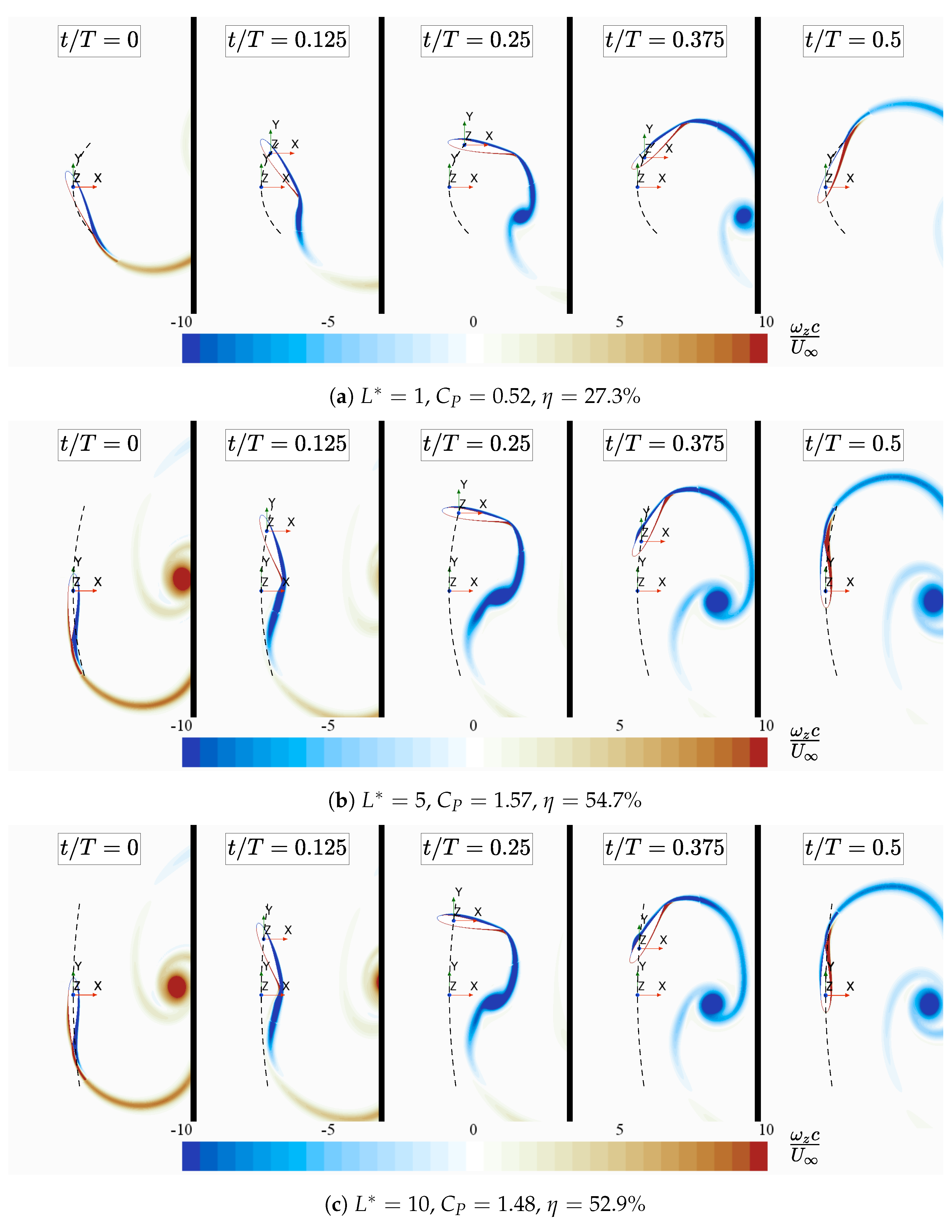
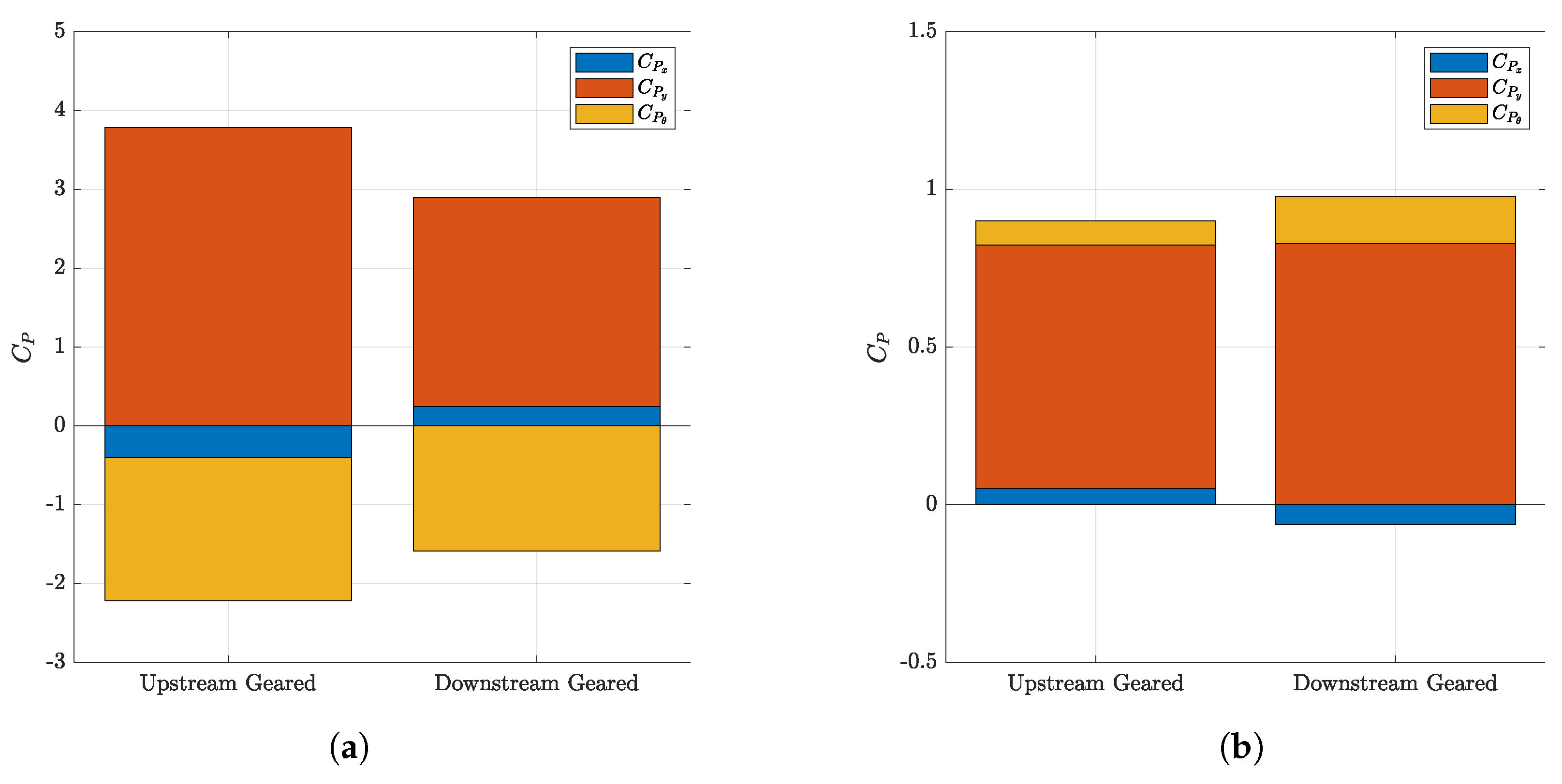
This paper presents an investigation of the energy harvesting potential of the fully passive oscillating-foil turbine on a swinging arm. This research was driven by the need to investigate different and simpler mechanical configurations than the fully passive oscillating-foil turbine on rails. Therefore, two different mechanisms, geared and gearless, were investigated in both downstream and upstream rest positions for different lengths of the swinging arm using 2D URANS CFD simulations. Furthermore, two different sets of optimized parameters yielding railed turbines operating under two different instability mechanisms, i.e., the coupled-flutter and stall-flutter instabilities, were used to establish equivalent parameters for the fully passive oscillating-foil turbines on a swinging arm of different lengths.

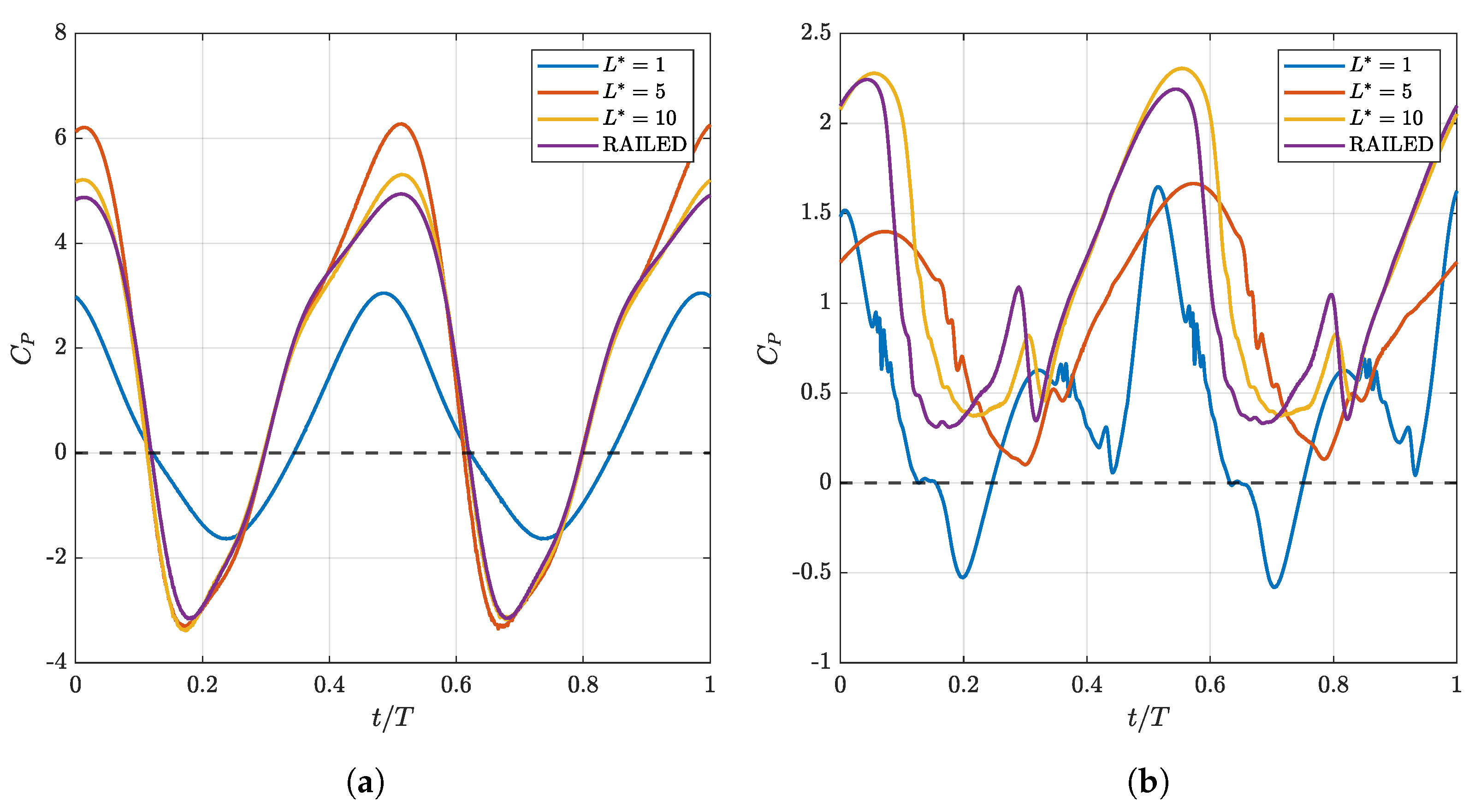
The results obtained are promising, showing that the fully passive oscillating-foil turbines on a swinging arm offer performances, i.e., efficiency values and power coefficients, comparable to or even better than those of the fully passive railed oscillating-foil turbines if the arm length is chosen carefully depending on the instability mechanism. For instance, when operating under the coupled-flutter instability and with the use of gears in an upstream configuration, an arm length of 5 chords offers a power coefficient and an efficiency value of $1.57$ and $54.7\%$, respectively. When compared to the fully passive railed oscillating-foil turbine, which has a power coefficient of $1.41$ and an efficiency value of $51.0\%$, the oscillating-foil turbine on a swinging arm therefore offers relatively similar performance metrics to those of the railed configuration, with increases of about $11\%$ and $7\%$, respectively. Such a configuration of the fully passive oscillating-foil turbine on a swinging arm would be a good prototype for experimental investigations.

Firstly, when operating under the coupled-flutter instability, the upstream configuration is always slightly better than its downstream counterpart, and the use of gears offers better performance metrics if the structural parameters of the railed configuration are scaled with respect to the arm length. Following this result, the initially unresponsive gearless model was adapted to become responsive and, thus, to provide viable performance metrics.

Secondly, it was found that both the geared and gearless configurations are well suited when the turbine is operating under the stall-flutter instability. Although intrinsically less efficient than when operating under the coupled-flutter instability, the robustness of the turbine when operating under the stall-flutter instability makes it suitable for use with all configurations analyzed, without requiring adjustment of the optimized railed structural parameters.

Therefore, given the current findings, a practical prototype should be based on the upstream geared configuration, operating under the coupled-flutter instability, with an arm length of more than five chords.

For future work, 3D simulations would provide insight into how such a turbine would operate when subjected to the tip effects of finite blade spans. An experimental study, as well as a sensitivity study, would also be very valuable to complement the simulations presented in this paper. It would also be of great interest to assess the performance of a turbine combining on the same arm the upstream and downstream FP-OFT-SA configurations in a tandem configuration. Some studies have looked into the fully-constrained and the semi- and fully-passive configurations in tandem configurations, showing strong interactions between the upstream foil’s wake and the downstream foil. However, most studies make use of an array of railed turbines rather than a single turbine consisting of two foils on a single rigid arm. Simulations using two fully-passive foils on a single arm might provide insight into whether greater power outputs and efficiency values can be reached if such tandem systems are carefully optimized. From an engineering point of view, building such a tandem apparatus seems to benefit from a swinging arm perspective. Indeed, it is a simpler solution than having two railed turbines in an array, and it permits a direct link between the heaving positions upstream and downstream, ensuring that both foils operate in a mirror pattern height-wise.

References

1. Xiao, Q.; Zhu, Q. A review on flow energy harvesters based on flapping foils. J. Fluids Struct. 2014, 46, 174–191. [Google Scholar] [CrossRef]
2. McKinney, W.; De Laurier, J. Wingmill: An Oscillating-Wing Windmill. J. Energy 1981, 5, 109–115. [Google Scholar] [CrossRef]
3. Young, J.; Lai, J.C.; Platzer, M.F. A review of progress and challenges in flapping foil power generation. Prog. Aerosp. Sci. 2014, 67, 27. [Google Scholar] [CrossRef]
4. Young, J.; Lai, J.; Platzer, M. Flapping foil power generation: Review and potential in pico-hydro application. In Proceedings of the 2015 International Conference on Sustainable Energy Engineering and Application (ICSEEA), Bangkok, Thailand, 25–26 October 2015; pp. 95–100. [Google Scholar] [CrossRef]
5. Wu, X.; Zhang, X.; Tian, X.; Li, X.; Lu, W. A review on fluid dynamics of flapping foils. Ocean. Eng. 2020, 195, 106712. [Google Scholar] [CrossRef]
6. Boudreau, M.; Gunther, K.; Dumas, G. Investigation of the energy-extraction regime of a novel semi-passive flapping-foil turbine concept with a prescribed heave motion and a passive pitch motion. J. Fluids Struct. 2019, 84, 368–390. [Google Scholar] [CrossRef]
7. Boudreau, M.; Picard-Deland, M.; Dumas, G. A parametric study and optimization of the fully-passive flapping-foil turbine at high Reynolds number. Renew. Energy 2020, 146, 1958–1975. [Google Scholar] [CrossRef]
8. Duarte, L.; Dellinger, N.; Dellinger, G.; Ghenaim, A.; Terfous, A. Flapping Foil Hydrokinetic Turbine: From a Strongly Coupled FSI Solver to the Experiment in a Confined Channel. In Advances in Critical Flow Dynamics Involving Moving/Deformable Structures with Design Applications; Braza, M., Hourigan, K., Triantafyllou, M., Eds.; Springer: Cham, Switzerland, 2021; pp. 315–325. [Google Scholar]
9. Duarte, L.; Dellinger, N.; Dellinger, G.; Ghenaim, A.; Terfous, A. Experimental investigation of the dynamic behaviour of a fully passive flapping foil hydrokinetic turbine. J. Fluids Struct. 2019, 88, 1–12. [Google Scholar] [CrossRef]
10. Duarte, L.; Dellinger, N.; Dellinger, G.; Ghenaim, A.; Terfous, A. Experimental optimisation of the pitching structural parameters of a fully passive flapping foil turbine. Renew. Energy 2021, 171, 1436–1444. [Google Scholar] [CrossRef]
11. Mann, S.; Dumas, G.; Oshkai, P. Confinement Effect on the Hydrodynamic Performance of a Fully-Passive Oscillating-Foil Turbine. Master’s Thesis, University of Victoria, Victoria, BC, Canada, 2022. [Google Scholar]
12. Gunther, K.; Mann, S.; Dumas, G.; Ohskai, P. Numerical and experimental comparison of confinement effects on a Fully-Passive Oscillating-Foil Turbine. In Proceedings of the Canadian Society for Mechanical Engineering International Congress, Edmonton, Alberta, 5–8 June 2022. [Google Scholar]
13. Lee, W.; Dumas, G.; Oshkai, P. Influence of the sweep angle on performance of a fully-passive oscillating-plate hydrokinetic turbine prototype. J. Fluids Struct. 2023, 125, 104048. [Google Scholar] [CrossRef]
14. Oshkai, P.; Iverson, D.; Lee, W.; Dumas, G. Reliability study of a fully-passive oscillating foil turbine operating in a periodically-perturbed inflow. J. Fluids Struct. 2022, 113, 103630. [Google Scholar] [CrossRef]
15. Theodorakis, K.; Ntouras, D.; Papadakis, G. Investigation of a submerged fully passive energy-extracting flapping foil operating in sheared inflow. J. Fluids Struct. 2021, 113, 103674. [Google Scholar] [CrossRef]
16. Goyaniuk, L.; Poirel, D.; Benaissa, A.; Amari, H. The energy extraction potential from pitch-heave coupled flutter. J. Sound Vib. 2023, 555, 117714. [Google Scholar] [CrossRef]
17. Gunther, K.; Genest, B.; Dumas, G. Efficient control of the fully passive oscillating foil in 2D confined flows with adjustment of the heave damping. AIP Adv. 2024, 14, 035041. [Google Scholar] [CrossRef]
18. Veilleux, J.C.; Dumas, G. Numerical optimization of a fully-passive flapping-airfoil turbine. J. Fluids Struct. 2017, 70, 102–130. [Google Scholar] [CrossRef]
19. Boudreau, M.; Dumas, G.; Rahimpour, M.; Oshkai, P. Experimental investigation of the energy extraction by a fully-passive flapping-foil hydrokinetic turbine prototype. J. Fluids Struct. 2018, 82, 446–472. [Google Scholar] [CrossRef]
20. Huxham, G.H.; Cochard, S.; Patterson, J. Experimental Parametric Investigation of an Oscillating Hydrofoil Tidal Stream Energy Converter. In Proceedings of the 18th Australasian Fluid Mechanics Conference, Launceston, Australia, 3–7 December 2012; p. 4. [Google Scholar]
21. Karbasian, H.; Esfahani, J.; Barati, E. The power extraction by flapping foil hydrokinetic turbine in swing arm mode. Renew. Energy 2016, 88, 130–142. [Google Scholar] [CrossRef]
22. Sitorus, P.E.; Ko, J.H. Power extraction performance of three types of flapping hydrofoils at a Reynolds number of 1.7E6. Renew. Energy 2019, 132, 106–118. [Google Scholar] [CrossRef]
23. Sitorus, P.E.; Le, T.Q.; Ko, J.H.; Truong, T.Q.; Park, H.C. Design, implementation, and power estimation of a lab-scale flapping-type turbine. J. Mar. Sci. Technol. 2016, 21, 115–128. [Google Scholar] [CrossRef]
24. Liu, Z.; Qu, H.; Shi, H. Energy-harvesting performance of a coupled-pitching hydrofoil under the semi-passive mode. Appl. Energy 2020, 267, 114889. [Google Scholar] [CrossRef]
25. Siemens Industries Digital Software, Simcenter STAR-CCM+, User Guide v.2021.2; Siemens: Munich, Germany, 2021.
26. Patankar, S.V. Numerical Heat Transfer and Fluid Flow; Series in Computational Methods in Mechanics and Thermal Sciences; McGraw-Hill [u.a.]: New York, NY, USA, 1980; pp. 189–193. [Google Scholar]
27. Anderson, J.D. Computational Fluid Dynamics; McGraw-Hill: New York, NY, USA, 1994; p. 547. [Google Scholar]
28. Olivier, M.; Paré-Lambert, O. Strong fluid–solid interactions with segregated CFD solvers. HFF 2019, 29, 2237–2252. [Google Scholar] [CrossRef]
29. Broyden, C.G. A class of methods for solving nonlinear simultaneous equations. Math. Comp. 1965, 19, 577. [Google Scholar] [CrossRef]
30. Spalart, P.; Rumsey, C. Effective Inflow Conditions for Turbulence Models in Aerodynamic Calculations. Am. Inst. Aeronaut. Astronaut. 2007, 45, 2544–2553. [Google Scholar] [CrossRef]
31. Jiang, W.; Zhang, D.; Xie, Y. Numerical investigation into the effects of arm motion and camber on a self-induced oscillating hydrofoil. Energy 2016, 115, 1010–1021. [Google Scholar] [CrossRef]
32. Polyak, B. Some methods of speeding up the convergence of iteration methods. Ussr Comput. Math. Math. Phys. 1964, 4, 1–17. [Google Scholar] [CrossRef]
33. Ruder, S. An overview of gradient descent optimization algorithms. arXiv 2016, arXiv:1609.04747. [Google Scholar] [CrossRef]
Figure 1. Schematic of the FP-OFT-SA in the (a) upstream and (b) downstream configurations. For simplicity, springs and dampers at pivots P and Q are not shown; valid with or without the geared mechanism.
Energies 18 01277 g001
Figure 2. Schematic representation of the equilibrium angular position β of the foil when the system is (a) geared and (b) gearless. Note that β corresponds to the resting position of the pitch spring in both configurations.
Energies 18 01277 g002
Figure 3. Schematic of the FP-OFT-SA in the upstream position (a) with and (b) without gears. Note that in (a), the pitch spring and damper were moved to a second set of gears and chain to facilitate comprehension of the illustration. In a real design, they could be superimposed to the arm’s spring and damper at point Q.
Energies 18 01277 g003
Figure 4. Trajectory of the FP-OFT (a) on rails and on a swinging arm in the (b) upstream and (c) downstream configuration; valid with or without the geared mechanism.
Energies 18 01277 g004
Figure 5. Height d of the energy extraction window of a FP-OFT-SA.
Energies 18 01277 g005
Figure 6. CFD domain and mesh for the FP-OFT-SA.
Energies 18 01277 g006
Figure 7. Instantaneous power coefficient of the FP-OFT-SA during a complete cycle as a function of the dimensionless length of the arm, using the upstream geared configuration and operating under (a) the coupled-flutter instability and (b) the stall-flutter instability.
Energies 18 01277 g007
Figure 8. Normalized vorticity ω z * = ω z c U field during half a cycle of the FP-OFT-SA, operating under the coupled-flutter instability in the upstream geared configuration with (a) L * = 1 , (b) L * = 5 and (c) L * = 10 . The arched heave motion is illustrated by the black dashed line.
Energies 18 01277 g008
Figure 9. Normalized vorticity ω z * = ω z c U field during half a cycle of the FP-OFT-SA, operating under the stall-flutter instability in the upstream geared configuration with (a) L * = 1 , (b) L * = 5 and (c) L * = 10 . The arched heave motion is illustrated by the black dashed line.
Energies 18 01277 g009
Figure 10. Power coefficient of the FP-OFT-SA as a function of the dimensionless length of the arm, operating under (a) the coupled-flutter instability and (b) the stall-flutter instability. The grey regions represent the standard deviation from the mean of the railed cases. The error bars of the data correspond to the standard deviation (SD).
Energies 18 01277 g010
Figure 11. Efficiency of the FP-OFT-SA as a function of the dimensionless length of the arm, operating under (a) the coupled-flutter instability and (b) the stall-flutter instability. The grey regions represent the standard deviation from the mean of the railed cases. The error bars of the data correspond to the standard deviation (SD).
Energies 18 01277 g011
Figure 12. Period of the FP-OFT-SA as a function of the dimensionless length of the arm, operating under (a) the coupled-flutter instability and (b) the stall-flutter instability. The grey regions represent the standard deviation from the mean of the railed cases. The error bars of the data correspond to the standard deviation (SD).
Energies 18 01277 g012
Figure 13. Extraction window height of the FP-OFT-SA as a function of the dimensionless length of the arm, operating under (a) the coupled-flutter instability and (b) the stall-flutter instability. The grey regions represent the standard deviation from the mean of the railed cases. The error bars of the data correspond to the standard deviation (SD).
Energies 18 01277 g013
Figure 14. Power coefficient comparison of the upstream and downstream geared configurations of the FP-OFT-SA with L * = 5 , operating under (a) the coupled-flutter instability and (b) the stall-flutter instability.
Energies 18 01277 g014
Figure 15. Instantaneous power coefficient of the adapted upstream gearless FP-OFT-SA during a complete cycle as a function of the dimensionless length of the arm using the coupled-flutter parameters.
Energies 18 01277 g015
Figure 16. Normalized vorticity ω z * = ω z c U field during half a cycle of the FP-OFT-SA, operating under the coupled-flutter instability in the adapted upstream gearless configuration with (a) L * = 2.5 , (b) L * = 5 and (c) L * = 10 . The arched heave motion is illustrated by the black dashed line.
Energies 18 01277 g016