Transient Equivalent Modelling of a Wind Farm Based on QPSO-Based Wind Turbine Fault Ride-Through Control

Abstract

At present, the equivalent modeling method of wind farms mostly adopts single-machine multiplication equivalence, which has the deficiencies of large model error and difficulty in accurately reflecting the fault transient characteristics of wind farms, which imposes limitations on the security and stability analysis of the power system. For this reason, this paper proposes an equivalent modeling method that can accurately reflect the fault ride-through characteristics of wind farms. Based on the control mechanism of direct-drive wind turbines, this method first analyzes the fault ride-through operating characteristics of wind turbines and establishes a single-machine fault transient model; then, taking the fault ride-through control characteristics of wind turbines as the criteria for subgroups, it calculates the relevant parameters of the group through weighted aggregation and QPSO algorithm, and constructs the fault transient equivalent model of each group; finally, combining with the principle of loss conservation, it integrates and obtains the fault transient equivalent model of the whole wind power field. Finally, the equivalent fault transient model of the whole wind farm is obtained by combining the loss conservation principle. Simulation verification shows that the established equivalent model can accurately reflect the dynamic characteristics of the wind farm, and the maximum percentage error of voltage and active power is no more than 10% in comparison with the corresponding detailed model under the same kind of fault perturbation, which not only meets the requirements of China’s wind farm modeling standards, but also shows higher adaptability and accuracy under different working conditions compared with other equivalent modeling methods. Especially under the extreme three-phase zero-passage fault condition, the maximum error of voltage and active power does not exceed 2%, which provides a reliable basic tool for the safety and stability analysis of wind farms.

1. Introduction

As large-scale wind farms interconnected in large areas gradually become the mainstream of wind power development, the study of the safety and stability of wind farms connected to the grid has become more and more important. In the simulation and analysis of wind farms, the traditional single-machine multiplication method has been widely used, but it has significant limitations when it cannot accurately reflect the complex interactions between wind farm units and the wake effect. In order to ensure the safe and stable operation of wind farms and improve the simulation accuracy, it has become a key issue to establish an equivalent model that can accurately reflect the characteristics of wind farms, especially the fault transient characteristics.

Large-scale wind farms usually contain hundreds to thousands of wind turbines, and if detailed transient modeling is carried out for each turbine, it is difficult for the existing computational capacity to meet the real-time simulation speed required for high-order models. Therefore, to address this problem, researchers have proposed a variety of simplified isotropic modeling methods, including the single-unit isotropic method, the semi-isotropic method, and the multi-machine isotropic method [1]. Among these, the multi-machine equivalence method has received widespread attention for its high accuracy, but its accuracy is highly dependent on the reasonable selection of subgroup indicators. The quantity and quality of the clustering indexes directly affect the error between the equivalence model and the detailed model; therefore, how to select appropriate clustering indexes, and especially how to improve the modeling accuracy under the consideration of the unit fault ride-through characteristics and the turbine wake effect, has become an important challenge to improve the accuracy of the model.

Tail current effect in wind farms is one of the key factors affecting modeling accuracy. Tail current interactions between wind turbines not only affect the power output, but also have a profound impact on the transient response of wind farms. Especially in large-scale wind farms, the wake effects between the turbines become more complicated with the increase of the number of turbines. If the wake effect is not fully considered in the modeling process, the simulation results will be difficult to accurately reproduce the dynamic performance of wind farms under faults or other complex operating conditions. Therefore, wind farm modeling should integrate the influence of wake effects to improve the accuracy and reliability of the model [2].

In addition, the control methods of wind farms play a decisive role in their overall performance and stability. In recent years, many emerging wind farm control techniques have been proposed to improve the energy yield efficiency of wind farms and to guarantee their stable operation. For instance, the Modified Sine Cosine Algorithm (M-SCA) has been successfully applied to optimize the controller parameters of wind turbines, significantly enhancing the total energy production of wind farms. This approach addresses the issue of wake interactions between turbines, which can degrade the overall energy output. The M-SCA modifies the standard Sine Cosine Algorithm (SCA) by introducing a nonlinear update mechanism and an average design variable, which helps to avoid premature convergence and improve the exploration and exploitation rates during the optimization process [3].

Furthermore, other advanced control techniques have been developed to enhance wind farm performance. For example, model-free closed-loop control methods with recursive least squares reinforcement learning have provided wind farms with smarter means of regulation, allowing for real-time adjustments based on environmental conditions [4]. Additionally, wind turbine yaw dynamics modeling has been widely used in active wind farm control to accurately regulate the operation of wind turbines, ensuring optimal alignment with wind direction and minimizing energy losses [5]. These advanced control techniques provide new perspectives for modeling wind farms, and the combination of these strategies helps to further improve the modeling accuracy and overall energy production.

Currently, several studies have proposed different clustering metrics for equivalent modeling of wind farms. The authors of [6], for wind farms with fixed wind speeds, obtained the wind turbine rotational speed by backward inverse extrapolation of the relevant parameters before and after the fault, then selected the wind turbine rotational speed at the instant of fault excision as a subgroup index for multi-machine modeling. The authors of [7] calculated the rotor current of the generator at the time of fault according to the parameters of the system operation state at the time of fault, combined with the principle of power balance, then selected the value of the rotor current of each machine at the time of fault as a subgroup index for modeling. The authors of [8] firstly used whether the chopper protection circuit was put into operation or not for grouping, then, on the basis of this, utilized the output voltage of the turbine which was not put into operation for chopper protection for grouping. The authors of [9] performed multi-machine equalization of wind farms based on the output active power of each wind turbine as a clustering index. The authors of [10] used a spectral clustering algorithm to cluster the wind turbines in a wind farm based on the operating status of each wind turbine in the wind farm. The authors of [11] extracted three dominant variables as clustering indexes among all state variables of WTGs based on principal component analysis. The authors of [12] established multiple clustering indicators for wind farms based on the operational characteristics of direct-drive WTGs. The authors of [13] proposed a two-step clustering method: firstly, whether the fault active power can be restored to the pre-fault value is taken as the clustering index, and all the units are divided into two clusters; then the clustering algorithm is utilized to further divide the clusters, in order to reduce the equalization error. Although these methods have improved the modeling accuracy to a certain extent, most of the studies have not fully considered the unit fault ride-through characteristics and the differences in the operation modes of the WTGs within the wind farms, which leads to the deviation between the equivalent model and the response of the actual wind farms in the fault ride-through process.

To address this issue, this paper proposes a multi-machine equivalent modeling method based on the fault ride-through control characteristic subgroup of direct-drive wind turbines. First, a single-machine fault transient model is constructed by analyzing the protection action characteristics of direct-drive wind turbines during the fault ride-through process. Then, based on the characteristics of the chopper protection and converter fault ride-through control actions of the units during wind farm faults, the units within the wind farm are grouped. By combining the existing single-machine fault transient model and the parameters of the units within each group, weighted aggregation and the QPSO algorithm are used to optimize the aggregated units. The QPSO algorithm possesses strong global optimization capabilities in multi-objective optimization problems and can effectively avoid local optima, making it particularly suitable for the optimization task of wind farm equivalent modeling [14,15,16].

Although QPSO is inherently random, we have implemented several measures to ensure the accuracy and reliability of the optimization results. First, during each optimization iteration, we calculated the corresponding loss value to evaluate the quality of the solution. To guarantee the validity of the optimization results, a predefined loss value threshold was set. Only results with a loss value below this threshold were considered valid. This approach effectively constrains the optimization parameters, ensuring that the final control parameters meet the required accuracy.

Furthermore, to address the randomness of QPSO, we conducted multiple optimization trials and performed a comprehensive statistical analysis on the results that met the loss value threshold. Specifically, we calculated the mean, standard deviation, and confidence intervals of the optimized parameters across all valid trials. The final optimization parameters were obtained by averaging the results from these trials. This statistical averaging process significantly reduces the uncertainty caused by the inherent randomness of QPSO, thereby improving the stability and reliability of the results.

Through repeated experiments and the application of the loss value threshold, we ensured that each optimization trial accurately reflects the system’s dynamic characteristics. The statistical averaging process further ensures parameter stability, making our approach suitable for practical applications where reliability and accuracy are critical.

Finally, the overall fault transient equivalent model of the wind farm was derived through the principle of power conservation, and its accuracy and adaptability were validated through simulations under various operating conditions.

A comparison of the methodology proposed in this paper with previous research results is shown in

Table 1. Comparative table of research methods.

Reference	Grouping Method	Limitations	Innovative Approach of This Paper
[6]	Wind turbine speed as a grouping index	Does not consider fault ride-through characteristics and operational mode differences of turbines	Combines fault ride-through characteristics and control action traits for more precise grouping
[7]	Rotor current values of the generator as a grouping index	Only considers system status during faults, without fault ride-through characteristics	Proposes a method of grouping based on control actions, accurately reflecting turbine fault ride-through behavior
[8]	Chopper protection circuit status as a grouping index	Does not account for response differences of various machine groups during faults	Grouping based on fault ride-through control characteristics for more detailed classification
[9]	Active power output as a grouping index	Does not fully consider turbine dynamics and fault ride-through behavior	Proposes a method based on control characteristics and protection mechanisms for better accuracy
[10]	Spectral clustering for grouping	Clustering process does not fully account for operational mode differences, leading to potential errors	Uses a more accurate grouping method based on control characteristics to reduce clustering errors
[11]	Principal component analysis to extract dominant variables for grouping	Does not consider turbine dynamic behavior during faults	Combines main circuit and control circuit parameters for multi-machine modeling, improving accuracy
[12]	Direct-drive turbine characteristics for grouping	Does not fully consider the impact of fault ride-through control on modeling accuracy	Proposes a new modeling approach integrating turbine fault ride-through control characteristics and grouping
[13]	Two-step grouping method	Does not explore the individual fault ride-through characteristics of turbines, which affects modeling accuracy	Proposes a more precise two-step grouping method combining fault ride-through characteristics

.

The multi-machine equivalent modeling method proposed in this paper can more accurately simulate the dynamic response of wind farms during faults, and improve the reliability and adaptability of the wind farm equivalent model. This method not only provides a theoretical basis for the safe and stable operation of wind farms, but also provides new technical support for the optimal scheduling and control of wind farms.

The contribution statement for this paper is as follows:

(1) A single-machine fault transient model is established by analyzing the protection action characteristics of direct-drive wind turbines during fault ride-through.

(2) The chopper protection and converter fault ride-through control action characteristics of the wind turbines within the wind farm are used as the basis for grouping, and the method of grouping wind farm units is refined.

(3) Weighted aggregation and QPSO algorithms are used to obtain the main circuit and control circuit parameters of each cluster, then the fault transient equivalent model is established.

(4) The method of obtaining the overall fault transient equivalent model of wind farm through the principle of power conservation is proposed, which further enhances the parameter accuracy of the model.

(5) The accuracy and adaptability of the model are verified by simulation under different working conditions, which ensures the simulation accuracy of the method for wind farm faults.

2. Detailed Modelling of Direct-Drive Wind Turbines

In this paper, the research idea of the equivalent modeling method for wind farms and the relationship between the models are as follows: (i) Detailed model of direct-drive wind turbine: Analyze the action characteristics of the protection control during fault traversal, which serves as the theoretical basis for the establishment of the equivalent transient model of direct-drive wind turbine and the equivalent transient model of the wind farm. (ii) Equivalent transient model of direct-driven wind turbine: Establish the fault transient model of a single turbine according to the action characteristics of protection control, which is used as the basis for the establishment of the internal group transient aggregation sub-model of the wind farm after sub-group equivalence. (iii) Transient aggregation sub-model of the internal group of wind farms: According to the differences in the action characteristics of the protection control, adopt the idea of multi-unit group equivalence to establish the transient aggregation sub-model of the internal group of machines. (iv) Equivalent transient model of wind farm: Establish the equivalent transient model of wind farm by synthesizing the transient aggregation sub-model of internal machine group of wind farm.

2.1. Structure and Working Principle of a Direct-Drive Wind Turbine

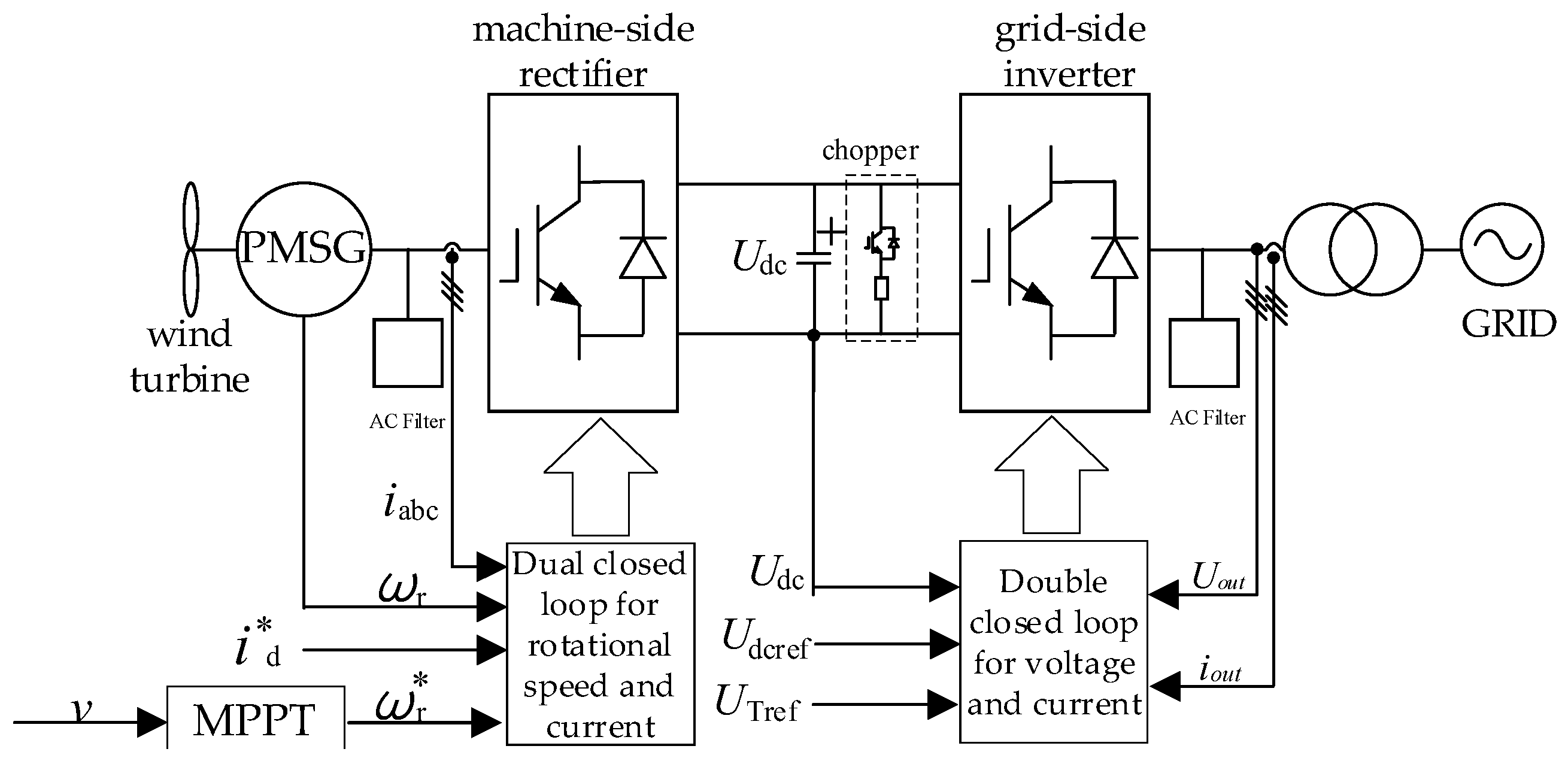
The WTG model and related parameters introduced in this project are provided by the project owner of Ningxia State Grid Electricity Academy; all types of units are WTG equipment that have been installed and actually put into operation in Ningxia regional power grid, and the mathematical models of the unit components are shown below. A direct-drive wind turbine mainly consists of a wind turbine, a permanent magnet synchronous generator, a back-to-back converter, a filter, and a chopper protection. The wind turbine and permanent magnet synchronous generator (PMSG) work together to convert wind energy into electricity. The back-to-back converter consists of a rectifier on the machine side and an inverter on the grid side, which is responsible for converting AC power with a variable frequency into AC power with a fixed frequency. The filter is used to filter out high-order harmonics caused by power electronic devices, while the chopper protection prevents the DC bus voltage from becoming too high.

The direct-drive wind turbine control system is divided into machine-side control and grid-side control. Machine-side control uses a dual-closed-loop control strategy based on rotor flux orientation for speed and current to achieve maximum wind energy tracking.

The grid-side control part adopts a voltage and current double-loop control strategy based on grid voltage orientation to ensure the stability of the DC bus voltage and regulate the grid-connected power, as shown in Figure 1.

2.2. Mathematical Model of a Direct-Drive Wind Turbine

The mathematical model of a direct-drive wind turbine mainly consists of a mechanical system model and an electrical system model. The mechanical system model only includes the aerodynamic model of the wind turbine, while the electrical system model mainly includes the electromagnetic model of the permanent magnet synchronous generator, the control model of the rectifier on the machine side, the control model of the inverter on the grid side, and the chopper overvoltage protection model.

2.2.1. Mechanical System Model

A wind turbine is a direct-drive wind turbine that captures wind energy. It consists of blades and a hub. Air flowing over the blades of the wind turbine generates aerodynamic forces that rotate the rotor of the wind turbine, converting wind energy into mechanical energy. Accurate mathematical modelling of wind turbines is complex and requires simplified analysis. Therefore, a simplified mechanical model of a wind turbine based on the blade element and the Bezier wind turbine momentum theory is as follows [17]:

$$\begin{array}{l}{P}_m={\displaystyle \frac{1}{2}}\rho \pi C_p\left(\lambda ,\beta \right)v^3{R}^2\\ T_m={\displaystyle \frac{P_m}{{\omega }_m}}={\displaystyle \frac{1}{2}}\rho \pi C_p\left(\lambda ,\beta \right)v^2{R}^3\\ C_p\left(\lambda ,\beta \right)=C_1\left({\displaystyle \frac{c_2}{{\lambda }_1}}-c_3\beta -c_4\right)e^{{\displaystyle \frac{-c_5}{{\lambda }_1}}}+c_6\lambda \\ {\displaystyle \frac{1}{{\lambda }_1}}={\displaystyle \frac{1}{\lambda +0.08\beta }}-{\displaystyle \frac{0.035}{{\beta }^3+1}}\end{array}$$

(1)

where P_m is the output power of the wind turbine, T_m is the output torque of the wind turbine, ρ is the air density, ν is the wind speed, R is the radius of the wind turbine rotor, ω_m is the mechanical angular velocity of the wind turbine, C_p(λ, β) is a function of the tip speed ratio λ and blade angle β, and c₁–c₆ are 0.5176, 116, 0.4, 5, 21, and 0.0068, respectively.

2.2.2. Electrical System Model

1.

Electromagnetic model of a permanent magnet synchronous generator

A permanent magnet synchronous generator (PMSG) is a low-speed synchronous generator that uses permanent magnets for excitation. Compared with traditional thermal synchronous generators, PMSGs are more efficient and have greater reliability and stability. This paper uses a hidden-pole PMSG for simplified modelling [18]. The general electromagnetic model of the PMSG under the d-q axis is obtained as follows:

$$\begin{array}{l}{\displaystyle \frac{d}{dt}}{i}_d={\displaystyle \frac{1}{L}}{\nu }_d-{\displaystyle \frac{R_s}{L}}{i}_d+n_p{\omega }_r{i}_q\\ {\displaystyle \frac{d}{dt}}{i}_q={\displaystyle \frac{1}{L}}{\nu }_q-{\displaystyle \frac{R_s}{L}}{i}_q+n_p{\omega }_r{i}_d-{\displaystyle \frac{{\psi }_r{n}_p{\omega }_r}{L}}\\ T_e=1.5{\psi }_r{n}_p{i}_q\end{array}$$

(2)

where: L represents the equivalent d and q axis inductances; R_s represents the stator winding resistance; i_d and i_q represent the stator d and q axis currents; v_d and v_q represent the stator d and q axis voltages; ω_r represents the rotor electrical angular velocity; ψ_r represents the magnetic flux linkage induced in the stator by the rotor permanent magnets; n_p represents the number of generator rotor pole pairs; and T_e represents the electromagnetic torque.

Controlling the q-axis current as the active current and the d-axis current as the reactive current, and making $e_d=0 , e_q={\psi }_r{n}_p{\omega }_r$, the equivalent circuit model of the permanent magnet synchronous generator in the d-q coordinate system is:

$$\begin{array}{l}{\nu }_d=L{\displaystyle \frac{d{i}_d}{dt}}+R_s{i}_d-L{n}_p{\omega }_r{i}_q+e_d\\ {\nu }_q=L{\displaystyle \frac{d{i}_q}{dt}}+R_s{i}_q-L{n}_p{\omega }_r{i}_d+e_q\end{array}$$

(3)

2.

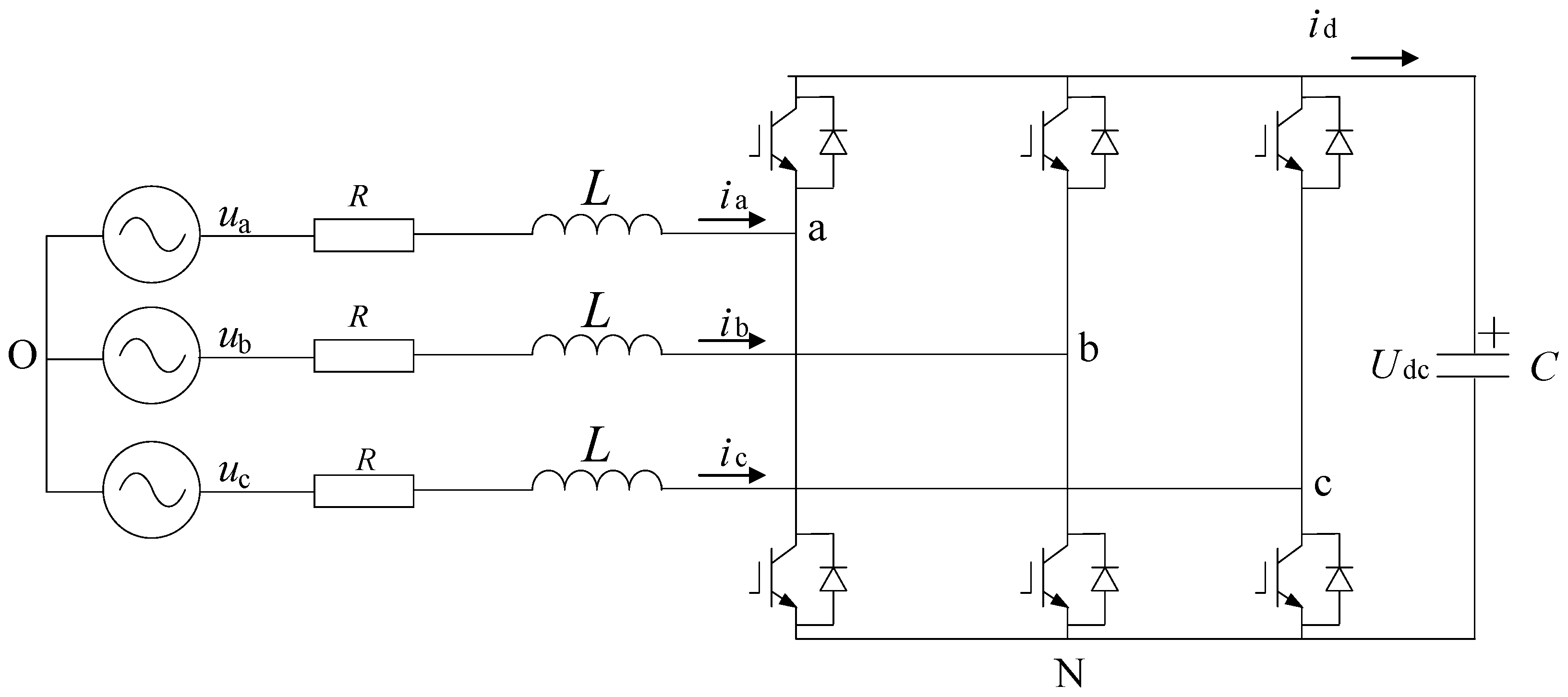
Machine-side rectifier model

The rectifier on the machine side uses the most common IGBT three-phase full-bridge rectifier. Its structure is a voltage rectifier, and its main function is to convert the variable-frequency AC power generated by the permanent magnet synchronous generator into DC power. The three-phase full-bridge rectifier circuit topology is shown in Figure 2.

Define the switching function of each bridge arm as S_n, where S_n takes on values either 0 or 1. According to the laws of KVL and KCL, the three-phase circuit equation of the full-bridge rectifier and the state equation of the DC-side capacitor are obtained as follows:

$$\begin{array}{l}{u}_a=L{\displaystyle \frac{d{i}_a}{dt}}+R_s{i}_a+\left(u_{aN}+u_{NO}\right)\\ u_b=L{\displaystyle \frac{d{i}_b}{dt}}+R_s{i}_b+\left(u_{bN}+u_{NO}\right)\\ u_c=L{\displaystyle \frac{d{i}_c}{dt}}+R_s{i}_c+\left(u_{cN}+u_{NO}\right)\\ i_d=S_a{i}_a+S_b{i}_b+S_c{i}_c\end{array}$$

(4)

Since u_nN = 0 when S_n = 0 and u_nN = U_dc when S_n = 1, u_nN = S_nU_dc; the equation for the three-phase circuit of the full-bridge rectifier can be rewritten as follows:

$$\begin{array}{l}{u}_a=L{\displaystyle \frac{d{i}_a}{dt}}+R_s{i}_a+\left(S_a{U}_{dc}+u_{NO}\right)\\ u_b=L{\displaystyle \frac{d{i}_b}{dt}}+R_s{i}_b+\left(S_b{U}_{dc}+u_{NO}\right)\\ u_c=L{\displaystyle \frac{d{i}_c}{dt}}+R_s{i}_c+\left(S_c{U}_{dc}+u_{NO}\right)\end{array}$$

(5)

Assuming that the permanent magnet synchronous generator outputs three-phase AC power with a balanced current, then:

$$\begin{array}{cc}\hfill u_{NO}& =-{\displaystyle \frac{1}{3}}{U}_{dc}\left(S_a+S_b+S_c\right)\hfill \\ & =-{\displaystyle \frac{1}{3}}{U}_{dc}{\displaystyle \sum _{n=a,b,c}{S}_n}\hfill \end{array}$$

(6)

The voltage, current and switching functions of the full-bridge rectifier in the three-phase coordinate system are transformed into the 3 s/2 r coordinate system to obtain the mathematical model of the three-phase full-bridge rectifier in the d-q rotating coordinate system. The transformation matrix of 3 s/2 r is:

$$T_{3s/2r}=\sqrt{{\displaystyle \frac{2}{3}}}\left[\begin{array}{ccc}cos\omega t& cos\left(\omega t-{\displaystyle \frac{2}{3}}\pi \right)& cos\left(\omega t+{\displaystyle \frac{2}{3}}\pi \right)\\ sin\omega t& sin\left(\omega t-{\displaystyle \frac{2}{3}}\pi \right)& sin\left(\omega t+{\displaystyle \frac{2}{3}}\pi \right)\\ {\displaystyle \frac{\sqrt{2}}{2}}& {\displaystyle \frac{\sqrt{2}}{2}}& {\displaystyle \frac{\sqrt{2}}{2}}\end{array}\right]$$

(7)

Substituting Equations (6) and (7) into Equation (5) of the circuit equation gives Equation (8), which is the mathematical model of the three-phase full-bridge rectifier on the machine side in the d-q rotating coordinate system:

$$\begin{array}{l}{u}_d=L{\displaystyle \frac{d{i}_d}{dt}}+R_s{i}_d+S_d{U}_{dc}-\omega L{i}_q\\ u_q=L{\displaystyle \frac{d{i}_q}{dt}}+R_s{i}_q+S_q{U}_{dc}+\omega L{i}_d\\ i_d=S_q{i}_d+S_d{i}_q\end{array}$$

(8)

where: u_d, u_q, i_d, and i_q are the voltage and current transformed from the three-phase stationary a-b-c coordinate system to the rotating d-q coordinate system; Sd and Sq are the switching functions of the bridge arm transformed from the three-phase stationary a-b-c coordinate system to the rotating d-q coordinate system; L and R_s are the internal inductance and stator winding resistance of the permanent magnet synchronous generator.

3.

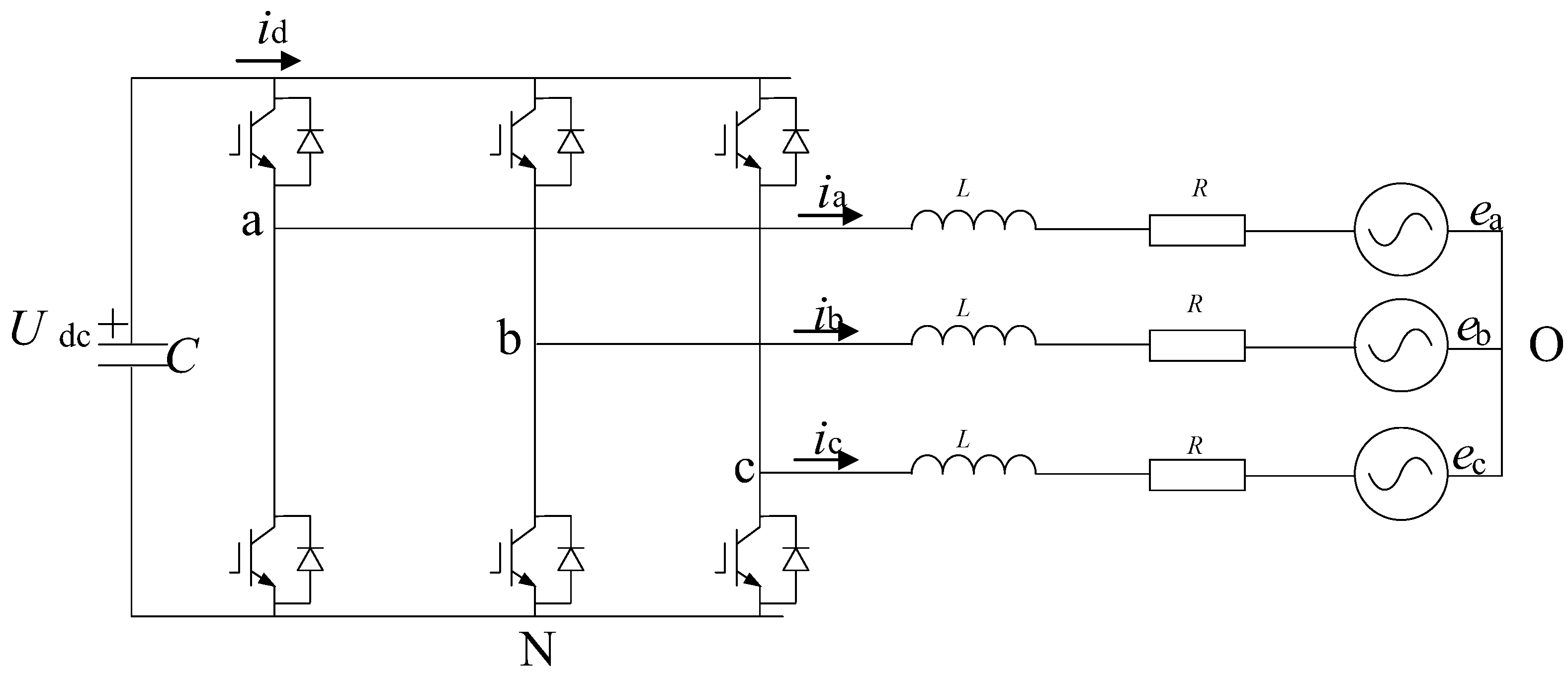
Grid-side inverter model

The grid-side inverter uses an IGBT three-phase full-bridge inverter, which has the same structure as the machine-side rectifier, but the direction of energy flow is opposite, and the switching function definition is the same as the machine-side rectifier. The three-phase full-bridge inverter circuit topology is shown in Figure 3.

The derivation of the mathematical model of a three-phase full-bridge rectifier is the same as that of a three-phase full-bridge inverter in the a-b-c three-phase coordinate system:

$$\begin{array}{l}{e}_a=\left(S_a-{\displaystyle \frac{1}{3}}{\displaystyle \sum _{n=a,b,c}{S}_n}\right)U_{dc}-L_e{\displaystyle \frac{d{i}_a}{dt}}-R_e{i}_a\\ e_b=\left(S_b-{\displaystyle \frac{1}{3}}{\displaystyle \sum _{n=a,b,c}{S}_n}\right)U_{dc}-L_e{\displaystyle \frac{d{i}_b}{dt}}-R_e{i}_b\\ e_c=\left(S_c-{\displaystyle \frac{1}{3}}{\displaystyle \sum _{n=a,b,c}{S}_n}\right)U_{dc}-L_e{\displaystyle \frac{d{i}_c}{dt}}-R_e{i}_c\end{array}$$

(9)

The mathematical model of a three-phase full-bridge inverter in the a-b-c three-phase coordinate system is transformed by 3 s/2 r coordinates, and the mathematical model of a three-phase full-bridge inverter in the d-q rotating coordinate system is obtained:

$$\begin{array}{l}{e}_d=S_d{U}_{dc}+\omega L_e{i}_q-L_e{\displaystyle \frac{d{i}_d}{dt}}-R_e{i}_d\\ e_q=S_q{U}_{dc}+\omega L_e{i}_d-L_e{\displaystyle \frac{d{i}_q}{dt}}-R_e{i}_q\end{array}$$

(10)

where: e_d, e_q, i_d, and i_q are the voltage and current in the rotating d-q coordinate system on the grid side; S_d and S_q are the switching functions of the bridge arm in the rotating d-q coordinate system on the grid side; and L_e and R_e are the grid-side filter inductance and grid connection line equivalent resistance.

2.3. Direct-Drive Wind Turbine Control Strategy

2.3.1. Machine-Side Control Strategy

In a direct-drive wind turbine, the back-to-back converter isolates the machine-side mechanical and electrical system from the power grid, so that the control objective of the machine-side part can remain unchanged throughout the entire operation. Normally, the control objective of the machine-side part is to maximize the wind turbine’s wind energy capture, which requires the rotor speed of the permanent magnet synchronous generator to stably and quickly track the optimal rotor speed of the wind turbine under different wind speeds.

For a generator, the rotor speed is controlled by the electromagnetic torque, which is often related to the rotor current. With a fixed power, the generator output voltage can be varied to control the rotor current, and thus the generator speed [19]. Therefore, the outer ring of the machine-side control part is the speed loop and the inner ring is the current loop.

The Laplace transform of Equation (3) gives the equation for current inner loop control:

$$\begin{array}{l}{\nu }_d=\left(k_c+k_{ci}{\displaystyle \frac{1}{s}}\right)\left(i_d^{*}-i_d\right)-L{n}_p{\omega }_r{i}_q\\ {\nu }_q=\left(k_c+k_{ci}{\displaystyle \frac{1}{s}}\right)\left(i_q^{*}-i_q\right)-L{n}_p{\omega }_r{i}_d+{\psi }_r{n}_p{\omega }_r\end{array}$$

(11)

where k_c and k_ci are the proportional integral parameters of the PI controller for the inner loop control of the motor-side current.

According to the generator electromagnetic torque equation and the speed control theory, the outer ring speed control equation is:

$$i_q^{*}=\left(k_v+k_{vi}{\displaystyle \frac{1}{s}}\right)\left({\omega }_r^{*}-{\omega }_r\right)$$

(12)

where k_v and k_vi are the proportional integral parameters of the PI controller for the outer ring speed control on the machine side.

The block diagram of the dual-closed-loop speed and current control based on the directional magnetic flux of the generator rotor, which is used in the side part of this machine, is shown in Figure 4. The control principle is to use the MPPT algorithm to calculate the optimal speed of the wind turbine, so that it can be used as the speed outer loop setting. The difference between the actual speed of the generator and the speed PI controller is used to obtain the current inner loop reference value $i_q^{*}$. The d-axis current reference value is set to 0, so that the q-axis current alone controls the generator torque. The current inner loop PI controller and the coupling term are then used to obtain the dq-axis control voltage. Finally, SVPWM modulation is used to generate the corresponding voltage PWM waveform. By controlling the conduction and switching of different IGBTs, the stator-side current can be adjusted, so that the inner loop current tracks the current setpoint and the outer loop speed tracks the speed reference value, thereby achieving maximum wind energy tracking for the wind turbine.

2.3.2. Network-Side Control Strategy

1.

Normal control strategy

During the operation of a direct-drive wind turbine, the DC bus voltage often fluctuates greatly due to the imbalance of wind power, which not only increases the risk factor of the DC bus capacitance, but also affects the amplitude of the inverter output voltage, posing a challenge to the stability of the wind turbine grid connection. At the same time, due to the large-scale penetration of wind power in recent years, the power grid requires wind turbines to have a high fault ride-through capability; that is, when a fault occurs at the grid connection point causing the grid-connected voltage to drop, the wind turbine must be able to output a certain amount of reactive power to restore the voltage.

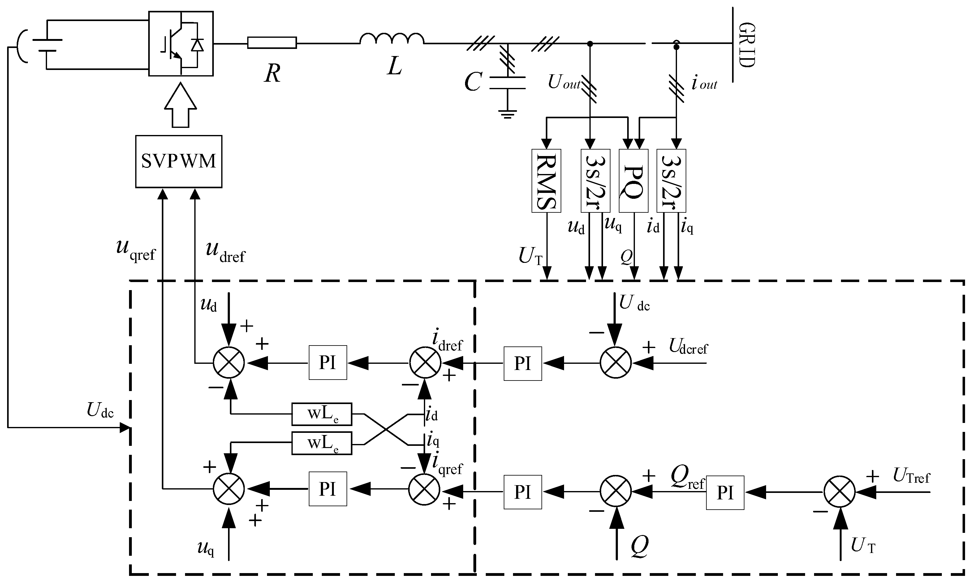
For this reason, grid-side inverters generally use a voltage and current double-loop control strategy based on grid voltage orientation. The outer loop control not only includes DC bus voltage control, but also reactive power control. The goal of the outer loop DC bus voltage control is to maintain a constant DC-side voltage, while the goal of reactive power control is to regulate the grid-connected power factor. The inner loop only includes current control, and the final output voltage is generated through current inner loop control and decoupling [20]. Therefore, the outer loop voltage and reactive power control equations are as follows:

$$\begin{array}{l}{Q}_{out}^{*}=\left(k_{p0}+{\displaystyle \frac{k_{i0}}{s}}\right)(U_{Tref}-U_T)\\ i_{dref}=\left(k_{p1}+{\displaystyle \frac{k_{i1}}{s}}\right)\left(U_{dcref}-U_{dc}\right)\\ i_{qref}=\left(k_{p2}+{\displaystyle \frac{k_{i2}}{s}}\right)\left(Q_{ref}-Q\right)\end{array}$$

(13)

where U_Tref and U_T are the set and measured values of the grid-side nominal voltage of the wind turbine; U_dc and U_dcref are the measured and reference values of the DC bus voltage; Q and Q_ref are the measured and reference values of the grid-side output reactive power, respectively; i_dref and i_qref are the reference values of the grid-side d-axis and q-axis currents, respectively; k_p0 and k_i0 are the coefficients of the PI controller for generating the reference reactive power; k_p1 and k_i1 are the PI controller coefficients of the outer loop of the d-axis voltage; and k_p2 and k_i2 are the PI controller coefficients of the outer loop of the q-axis reactive power.

The Laplace transform of Equation (10) gives the inner loop control equation for the current:

$$\begin{array}{l}{u}_{dref}=\left(k_{p3}+{\displaystyle \frac{k_{i3}}{s}}\right)\left(i_{dref}-i_d\right)-\omega L_e{i}_q+u_d\\ u_{qref}=\left(k_{p3}+{\displaystyle \frac{k_{i3}}{s}}\right)\left(i_{qref}-i_q\right)+\omega L_e{i}_d+u_q\end{array}$$

(14)

where u_dref and u_qref are the reference values of the d-axis and q-axis voltages output by the grid-side inverter, respectively; i_d and i_q are the real-time values of the d-axis and q-axis currents output by the grid-side, respectively; u_d and u_q are the real-time values of the d-axis and q-axis voltages output by the grid-side, respectively; and k_p3 and k_i3 are the coefficients of the PI controller of the grid-side current inner loop.

When the system is operating normally, the setting of the reactive power outer ring on the grid side is set to 0. When the system enters fault ride-through mode, the setting of the reactive power outer ring on the grid side is changed so that the q-axis current output by the outer ring at this time is the reference value of the reactive current under the specified high fault ride-through control. The simplified normal control topology on the grid side is shown in Figure 5.

2.

Fault ride-through control strategy

When the system detects a voltage sag/swell fault, the system will switch the control model in real time according to the voltage sag/swell level. In the initial moment of a fault, the voltage deviation is small, and the initial fault voltage is generally greater than 0.9 pu or less than 1.1 pu. At this time, the grid side still uses the normal control strategy to output active and reactive power. When the fault voltage continues to drop or rise, causing the grid voltage to drop below 0.9 pu or rise above 1.1 pu, the grid side control switches to the fault control strategy. At this time, the grid side’s previously normally controlled voltage and reactive power outer loop first remove their respective integral links, initially enhance the tracking speed of the reactive power of the outer loop, and reduce the outer loop regulation time. At the same time, in order to reduce the reactive current error caused by the single-proportional fault ride-through control loop, a certain reactive current difference needs to be compensated to ensure that the reactive current of the fault ride-through reactive outer loop control output can reach the specified value.

2.4. Fault Ride-Through Protection for Direct-Drive Wind Turbines

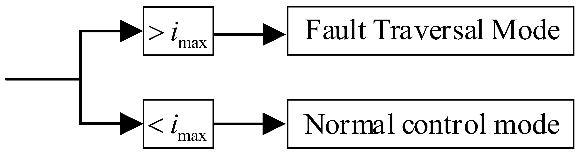
Fault ride-through control protection switching judgment control is shown in Figure 6. In order to avoid overcurrent damage to the grid-side converter of a direct-drive wind turbine, the grid-side converter usually limits the maximum converter current to 1.1–1.2 pu. When the current reaches the limit value, the drop is very close to the fault ride-through starting voltage. Therefore, it can be considered that the input of the converter fault ride-through control is related to whether the output current of the grid-side converter reaches the limiting value. When the grid-side output current reaches the maximum limiting current of the grid-side converter, the fault ride-through control protection is enabled, otherwise it is not enabled.

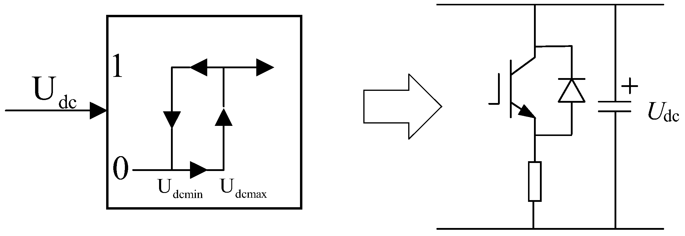
The chopper protection switching judgment control is shown in Figure 7. To prevent overvoltage of the DC bus capacitor, chopper protection is provided on both sides of the DC bus capacitor. Chopper protection switching generally uses hysteresis control. When the DC bus voltage exceeds the maximum operating voltage U_dcmax, the chopper is engaged, and when the DC bus voltage is lower than the minimum operating voltage U_dcmin, the chopper is disconnected [21].

During normal operation, the input and output of the wind turbine maintain power balance, the DC bus capacitor voltage does not exceed the chopper protection operating voltage U_dcmax, and the grid-side inverter output current does not exceed the maximum converter current value I_max. Neither the chopper protection nor the converter fault ride-through control is activated. When there is a grid-connected fault with the wind turbine, the system power balance is disrupted, the DC bus capacitor voltage and grid-side output current change, and the system chopper protection and converter fault ride-through control status will also change accordingly [22,23,24,25].

Due to the difference in the input value and control mode of the protective actions of the two, the action time of the chopper protection and the converter fault ride-through control during a fault will also be different, making the fault process of the unit appear to have the effect of multi-modal series connection. According to the combination of the action states of the chopper protection and the converter fault ride-through control, the entire transient fault process of the unit can be divided into four states. The multi-modal transient faults of the unit are shown in

Table 2. Multi-modal division of unit fault transients.

	Chopper Input	Chopper Not Engaged
Fault ride-through control is engaged	Chopper and fault ride-through control are both active	Chopper not engaged; fault ride-through control engaged
Fault ride-through control not implemented	Chopper input, fault ride-through control not engaged	Chopper and fault ride-through control are not engaged

.

2.5. Fault Transient Model of a Direct-Drive Wind Turbine

This section is based on the idea of using a chopper and a fault ride-through control to segmentally analyze the fault transient characteristics, as proposed in [26]. A simplified reduced-order analysis is performed on the detailed model of a wind turbine with complex fault ride-through control, thereby constructing a method for building a fault transient model for a direct-drive wind turbine. The simplified model is modelled as follows.

Wind turbines are usually regarded as low-pass wind speed filters with large filter time constants. When the wind speed fluctuates greatly, the wind turbine can adjust the angle or speed of the blades through its internal control system, thereby reducing the rapidly changing high-frequency components and outputting a more stable wind speed. Moreover, the transient time of a unit fault is generally in the millisecond range, so it can be considered that the wind speed is fixed during the transient process, and the input power of the unit will also be a fixed power value [27]. Based on the relationship between output voltage, current, and apparent power, the expression of the output voltage during the transient state of a unit fault is derived as follows:

$$U_{out}={\displaystyle \frac{P_{out}+j{Q}_{out}}{I_{out}^{*}}}$$

(15)

where P_out and Q_out are the active and reactive powers output from the wind turbine side of the network, respectively; and $I_{\mathit{out}}^{*}$ and U_out are the conjugate current vector and fault voltage vector output from the wind turbine side of the network during a fault, respectively.

From Equation (15), it can be seen that the transient output voltage of the wind turbine fault is controlled by the output power and current of the unit. However, the switching of the wind turbine chopper protection and fault ride-through control protection will directly affect the output power and current of the wind turbine. Therefore, it is first necessary to derive the output power and current of the wind turbine under the switching of the chopper protection and fault ride-through control protection.

1.

Chopper protection not engaged

The expression for the active power output of the wind turbine when the chopper protection is not engaged is:

$$P_{out}=P_{in}-0.5C{\displaystyle \frac{d{u}_{dc}^2}{dt}}$$

(16)

where P_in is the input power of the unit, which will also be a fixed value due to the fixed wind speed; C is the DC bus capacitor.

2.

Chopper protection input

The expression for the output active power when the wind turbine’s chopper protection is engaged is:

$$P_{out}=P_{in}-0.5C{\displaystyle \frac{d{U}_{dc}^2}{dt}}-{\displaystyle \frac{U_{dc}^2}{R_c}}$$

(17)

where R_c is the discharge resistor of the chopper protection circuit.

3.

Normal control mode

In order to ensure the stability of the DC bus voltage and the adjustable output power factor of the wind turbine generator, the grid-side converter usually adopts voltage-reactive outer-loop PI and current inner-loop PI control based on grid voltage orientation. However, the control time scale of the inner loop is generally designed to be much smaller than that of the outer loop. Therefore, when the wind turbine generators are operating normally or are only slightly affected by faults and have not entered fault ride-through control, the default current inner loop can quickly track the current reference value during the transient time; that is, it can be considered that the actual output current on the grid side will be equal to the current value output by the outer loop. The inner loop reference current expression is shown in Equation (13).

The reactive outer loop of the grid-side voltage also uses classic PI control, in which the integral link can eliminate errors but also correspondingly reduces the control speed. Considering the transient nature of the system fault ride-through process, the control of the outer loop integral can be ignored within the allowable error range, so that the actual output dq current of the grid side is approximately equal to the inner loop reference current value output under simplified outer loop proportional control. The inner loop reference current expression that ignores the integral link is as follows:

$$\left\{\begin{array}{l}{Q}_{out}^{*}=k_{p0}(1-U_T)\\ i_{drel}=i_d^{*}=k_{p1}(U_{dc}^{*}-U_{dc})\\ i_{qrel}=i_q^{*}=k_{p2}(Q_{out}^{*}-Q_{out})\end{array}\right.$$

(18)

4.

Fault ride-through control protection mode

When the wind turbine is greatly affected by a fault and the output current on the grid side rises to the maximum current limit of the grid-side converter, the grid-side converter enters fault ride-through control. At this time, the reference value of the dynamic reactive current in the inner loop of the grid-side control will be directly set according to the provisions of GB/T19963.1-2021 [28]. The expressions for setting the active and reactive current references are as follows:

$$\left\{\begin{array}{l}{i}_{qref}=1.5(0.9-U_T)I_N\\ i_{dref}=\sqrt{I_{max}^2-i_{qref}^2}\end{array}\right.$$

(19)

where I_N is the rated output current of the wind turbine generator and I_max is the maximum amplitude current of the grid-side converter.

According to the given active and reactive current values specified in the national standard, outer loop proportional control that ignores the integral link, and the set compensation link, the inner loop reference current expression under fault ride-through control can be obtained as follows:

$$\left\{\begin{array}{l}{Q}_{out}^{*}=k_{p0}(1-U_T)\\ i_{dref}=i_d^{*}=k_{p1}(U_{dc}^{*}-U_{dc})\\ i_{qref}^{*}=i_q^{*}=k_{p2}(Q_{out}^{*}-Q_{out})\\ i_{qref}=i_{qref}^{*}+i_{qref\_dip}\end{array}\right.$$

(20)

where i_{qref_dip} is the reactive current compensation term of the reactive external loop under fault ride-through control and $i_{\mathit{qref}}^{*}$ is the reactive current output of the reactive external loop under fault ride-through control.

Based on the above analysis of the output power and current under the chopper protection and fault ride-through control protection switching, the power and current expressions of the wind turbine in the four possible modes during a fault condition can be obtained. For details, see

Table 3. Output expression under multimodal condition of unit failure.

Modal	Chopper and Fault Ride-Through Control Are Not Engaged	Chopper Not Engaged Fault Ride-Through Control Engaged
${\mathrm{P}}_{\mathrm{out}}$	${\mathrm{P}}_{\mathrm{in}}-0.5\mathrm{C}{\displaystyle \frac{{\mathrm{du}}_{\mathrm{dc}}^2}{\mathrm{dt}}}$	${\mathrm{P}}_{\mathrm{in}}-0.5\mathrm{C}{\displaystyle \frac{{\mathrm{du}}_{\mathrm{dc}}^2}{\mathrm{dt}}}$
${\mathrm{Q}}_{\mathrm{out}}$	${\mathrm{Q}}_{\mathrm{out}}^{*}-{\displaystyle \frac{{\mathrm{i}}_{\mathrm{qrel}}}{{\mathrm{k}}_{\mathrm{p}2}}}$	${\mathrm{Q}}_{\mathrm{out}}^{*}-{\displaystyle \frac{{\mathrm{i}}_{\mathrm{qref}}}{{\mathrm{k}}_{\mathrm{p}2}}}$
${\mathrm{I}}_{\mathrm{out}}^{*}$	${\mathrm{i}}_{\mathrm{drel}}{+\mathrm{ji}}_{\mathrm{qrel}}$	${\mathrm{I}}_{\max }$
modal	Chopper input fault ride-through control not engaged	Chopper and fault ride-through control are both active
${\mathrm{P}}_{\mathrm{out}}$	${\mathrm{P}}_{\mathrm{in}}-0.5\mathrm{C}{\displaystyle \frac{{\mathrm{du}}_{\mathrm{dc}}^2}{\mathrm{dt}}}-{\displaystyle \frac{{\mathrm{u}}_{\mathrm{dc}}^2}{{\mathrm{R}}_{\mathrm{c}}}}$	${\mathrm{P}}_{\mathrm{in}}-0.5\mathrm{C}{\displaystyle \frac{{\mathrm{du}}_{\mathrm{dc}}^2}{\mathrm{dt}}}-{\displaystyle \frac{{\mathrm{u}}_{\mathrm{dc}}^2}{{\mathrm{R}}_{\mathrm{c}}}}$
${\mathrm{Q}}_{\mathrm{out}}$	${\mathrm{Q}}_{\mathrm{out}}^{*}-{\displaystyle \frac{{\mathrm{i}}_{\mathrm{qref}}}{{\mathrm{k}}_{\mathrm{p}2}}}$	${\mathrm{Q}}_{\mathrm{out}}^{*}-{\displaystyle \frac{{\mathrm{i}}_{\mathrm{qrel}}}{{\mathrm{k}}_{\mathrm{p}2}}}$
${\mathrm{I}}_{\mathrm{out}}^{*}$	${\mathrm{I}}_{\max }$	${\mathrm{i}}_{\mathrm{drel}}{+\mathrm{ji}}_{\mathrm{qrel}}$

.

Substituting the expressions for active power, reactive power and current in each mode into Equation (15), the transient output voltage of the generator set in different modes can be obtained, as shown in Equation (21).

$$U=\left\{\begin{array}{cc}{\displaystyle \frac{2}{3}}\times {\displaystyle \frac{P_{in}+\frac{C}{k_{p1}}\left(U_{dc}^{*}-\frac{i_{drel}}{k_{p1}}\right)\frac{d{i}_{drel}}{dt}+j\left(Q_{out}^{*}-\frac{i_{qrel}}{k_{p2}}\right)}{i_{drel}-j{i}_{qrel}}}& i_{rel}<i_{max},U_{dc}<U_{dcmax}\\ {\displaystyle \frac{2}{3}}\times {\displaystyle \frac{P_{in}+\frac{C}{k_{p1}}\left(U_{dc}^{*}-\frac{i_{dref}}{k_{p1}}\right)\frac{d{i}_{dref}}{dt}+j\left(Q_{out}^{*}-\frac{i_{qref}^{*}}{k_{p2}}\right)}{i_{dref}-j{i}_{qref}}}& i_{rel}\ge i_{max},U_{dc}<U_{dcmax}\\ {\displaystyle \frac{2}{3}}\times {\displaystyle \frac{P_{in}+\left(\frac{C}{k_{p1}}\frac{d{i}_{drel}}{dt}+\frac{U_{dc}^{*}-\frac{i_{drel}}{k_{p1}}}{R_c}\right)\left(U_{dc}^{*}-\frac{i_{drel}}{k_{p1}}\right)+j\left(Q_{out}^{*}-\frac{i_{qrel}}{k_{p2}}\right)}{i_{drel}-j{i}_{qrel}}}& i_{rel}<i_{max},U_{dc}\ge U_{dcmax}\\ {\displaystyle \frac{2}{3}}\times {\displaystyle \frac{P_{in}+\left(\frac{C}{k_{p1}}\frac{d{i}_{dref}}{dt}+\frac{U_{dc}^{*}-\frac{i_{dref}}{k_{p1}}}{R_c}\right)\left(U_{dc}^{*}-\frac{i_{dref}}{k_{p1}}\right)+j\left(Q_{out}^{*}-\frac{i_{qref}^{*}}{k_{p2}}\right)}{i_{dref}-j{i}_{qref}}}& i_{rel}\ge i_{max},U_{dc}\ge U_{dcmax}\end{array}\right.$$

(21)

As can be seen from Equation (21), the multimode of the wind turbine fault transient process can be equivalently represented as a controlled voltage source. At a fixed input power, the wind turbine fault transient output voltage is not only related to the grid-side reactive power and the DC bus voltage reference value, but also to the proportional coefficient of the grid-side control part and the output current.

3. QPSO-Based Equivalent Modelling of Wind Farm Transients

3.1. Equivalent Total Steps of Wind Farm Fault Transients

Usually, there are hundreds of direct-drive wind turbines inside a direct-drive wind farm. In order to fully capture the wind energy, the turbines inside are generally distributed in a decentralized manner. However, due to the wake effect of the wind farm, the wind speed inside the wind farm is unevenly distributed. At the same time, considering the difference in the distance between each turbine inside the wind farm and the fault point of the wind farm, these all lead to the fact that when a fault occurs at the grid-connected part of the wind farm, the transient response modes of each turbine inside are also different [29,30]. Therefore, in this section, the differences in the modes of the wind turbines during a fault and the similarities in the fault characteristics are used to establish a more simplified equivalent transient model for the wind farm based on the fault transient model of the wind turbine and using the method of grouping multiple machines into equivalent groups.

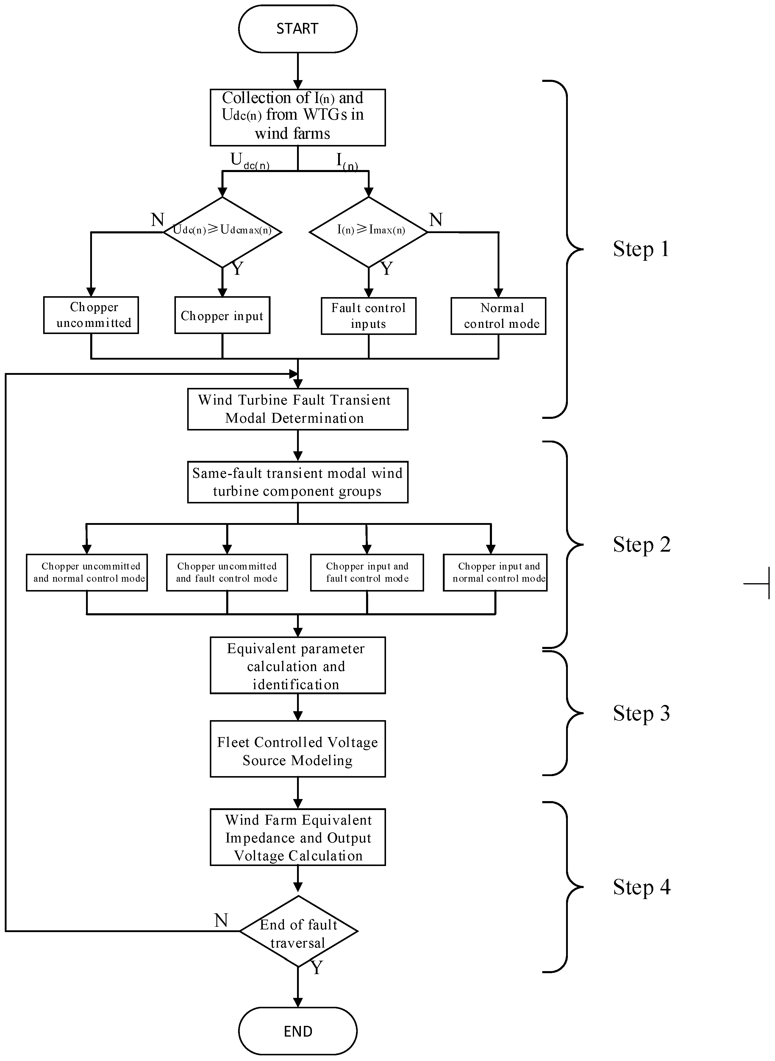
Figure 8 shows the equivalent steps of the wind farm fault transient model. In this paper, chopper protection and grid-side converter fault ride-through control are selected as indicators for modal grouping of wind turbines within the wind farm. Then, the circuit and control parameters of each modal group are obtained by means of single-machine equivalence and parameter identification. The equivalent single wind turbine of the same modal group is obtained, and the fault transient output voltage of the modal group is obtained based on this. Finally, the power balance principle is used to obtain the fault transient model of the wind farm. The steps for modelling the wind farm transient are as follows:

Step 1: Collect the grid-side output current I_(n) and DC-link capacitive voltage U_dc(n) of each wind turbine in the wind farm. Based on the collected DC-link capacitive voltage and output current, and combined with the set chopper protection circuit operating voltage U_dcamx(n) and converter maximum amplitude current value i_max(n) of each unit, determine the fault operation mode of each wind turbine, where n represents the nth unit in the wind farm.

Step 2: Group the wind turbines within the wind farm according to whether the chopper is operating and whether the grid-side converter is controlled by fault ride-through. Group the wind turbines that are in the same operating mode at the same time during a fault into the same group. In total, all wind turbines within the wind farm may be divided into four groups, namely: groups with both the chopper and converter fault ride-through controls active, groups with the converter fault ride-through control active and the chopper not active, groups with the chopper active and the converter fault ride-through control not active, and groups with both the chopper and converter fault ride-through controls active.

Step 3: Determine the aggregated units contained in each fleet, collect the basic parameters and fault measurement data of each unit. According to the basic parameters of the wind turbines under the jurisdiction of each fleet, the basic parameter value of the aggregated fleet is calculated by averaging or weighted averaging, then the quantum particle swarm recognition algorithm is used with the measured data to obtain the key equivalent parameters required for aggregation. Then, the grouped fleets are each equivalent to independent wind turbines, and the relevant parameters are substituted into the formula to calculate the transient fault output voltage U_(N) of the fleets in different modes. Finally, the fleet transient model can be temporarily equivalent to a model of multiple controlled voltage sources.

Step 4: Calculate the total collector line impedance Z of the wind farm based on the equivalent line impedance Z_(N) of the fleet obtained in step 3, and calculate the fault output voltage U of the wind farm transient model using the transient fault output voltage and equivalent current of the fleet in step 3, so as to finally equate the wind farm transient model to a controlled voltage source model.

In addition, as the fault continues, the failure mode of the wind turbines within the wind farm will change over time. Therefore, during the fault transient process of the wind farm, repeated cycling is required to perform clustering equalization until the fault transient process ends and the clustering equalization can be completed.

3.2. Aggregation of Basic Parameters of Wind Farm Fault Transient Equivalent Machine Group

In step 3, each group of machines is modelled as an equivalent single machine based on the single-machine fault transient voltage source model. In the process, the equivalent output voltage of the fault transient state needs to be calculated, so the equivalent aggregation and identification of the basic parameters and key control parameters of the group of machines must be carried out [31,32]. The equivalent basic parameters of the fleet that need to be aggregated mainly include: the reference value of the equivalent DC bus capacitive voltage, the equivalent DC bus capacitance, the equivalent impedance of the fleet collector circuit, and the equivalent active power input value of the fleet machine side. The key control parameters mainly include the proportional coefficients of the reference reactive power generation loop, the outer loop proportional coefficients of the d-axis voltage, and the outer loop proportional coefficients of the q-axis reactive power ${\overline{k}}_{p0}$, ${\overline{k}}_{p1}$, and ${\overline{k}}_{p2}$.

Considering that the magnitude of the output current on the network side is similar to the reference value of the capacitive voltage of the station unit, the reference value of the equivalent capacitive voltage $U_{dc(N)}^{*}$ of the fleet’s DC bus is approximately expressed as the average value of the reference value of the capacitive voltage of the fleet’s DC bus. The calculation formula is as follows:

$$U_{dc(N)}^{*}={\displaystyle \frac{1}{k_N}}{\displaystyle \sum _{j=1}^{k_N}{U}_{dc(j)}^{*}}$$

(22)

where $U_{dc(j)}^{*}$ is the reference value of the DC bus voltage of a single wind turbine included in fleet N; N represents the four types of fleets within the wind farm, N = 1, 2, 3, 4; k_N represents the number of wind turbines in fleet N after grouping; and j represents a single wind turbine included in fleet N.

Considering the superimposed power borne by the aggregated DC bus, the equivalent capacitance $\overline{C}$ of the DC bus of the fleet can be approximately expressed as the sum of the capacitance of the DC bus of all units in the fleet. The calculation formula is as follows:

$$\stackrel{-}{C}={\displaystyle \sum _{j=1}^{k_N}{C}_j}$$

(23)

where $C_j$ represents the DC bus capacitance value of a single wind turbine included in fleet N.

Considering that the impedance of the collector line should be calculated according to the principle of consistent losses before and after the equivalent, the equivalent impedance Z_(N) of the collector line of the fleet can be obtained by weighted aggregation. The calculation formula is as follows:

$$\begin{array}{l}{Z}_{(N)}={\displaystyle \frac{{\displaystyle \sum _{j=1}^{k_N}{i_{N(j)}}^2}{Z}_{(j)}}{{i_{N(N)}}^2}}\\ i_{N(N)}={\displaystyle \sum _{j=1}^{k_N}{i}_{N(j)}}\end{array}$$

(24)

where Z_(j) is the collector circuit impedance of the single wind turbine included in fleet N; i_N(j) is the rated current of the single wind turbine included in fleet N; and i_N(N) is the equivalent rated current of fleet N.

Considering the isolation effect of the fault process converter and the inertial characteristics of the wind turbine, it can be assumed that the input power on the machine side of the unit remains unchanged. Therefore, the equivalent active power input value $P_{in(N)}^{*}$ on the machine side of the fleet can be approximately expressed as the sum of the input powers on the machine side of all units in the fleet, and the calculation formula is as follows:

$$P_{in(N)}^{*}={\displaystyle \sum _{j=1}^{k_N}{P}_{in(j)}^{*}}$$

(25)

where $P_{in(j)}^{*}$ represents the active power input value on the machine side of a single wind turbine included in fleet N.

3.3. Identification of Key Control Parameters for QPSO-Based Fault Transient Equivalent Machine Groups

The main processes for identifying the key control parameters of the equivalent fleet include determining the objective function, selecting measured data, and iterative training of intelligent algorithms to obtain the optimal fleet equivalent parameters [33]. The control model to be recognized is shown below:

$$\left\{\begin{array}{l}{Q}_{out(N)}^{*}={\stackrel{-}{k}}_{p0}(1-U_{T(N)})\\ i_{dre{f}_{(N)}}=i_{d(N)}^{*}={\stackrel{-}{k}}_{p1}(U_{{}_{dc}(N)}^{*}-U_{dc(N)})\\ i_{qre{f}_{(N)}}^{*}=i_{q(N)}^{*}={\stackrel{-}{k}}_{p2}(Q_{out(N)}^{*}-Q_{out(N)})\end{array}\right.$$

(26)

where the parameters related to each input data in the identification model are calculated as follows:

$$\left\{\begin{array}{l}{Q}_{out(N)}^{*}={\displaystyle \sum _{j=1}^{k_N}{Q}_{out(j)}^{*}}\\ U_{dc(N)}={\displaystyle \frac{1}{k_N}}{\displaystyle \sum _{j=1}^{k_N}{U}_{dc(j)}}\\ i_{qre{f}_{(N)}}^{*}=i_{qre{f}_{(N)}}-i_{qref\_dip(N)}\\ i_{dre{f}_{(N)}}=\sqrt{{\left({\displaystyle \sum _{j=1}^{k_N}{I}_{max(j)}}\right)}^2-i_{qre{f}_{(N)}}^2}\\ i_{qre{f}_{(N)}}={\displaystyle \sum _{j=1}^{k_N}1.5\left(0.9-U_{T(j)}\right)g{I}_{N(j)}}\\ I_{N(j)}={\displaystyle \frac{P_{(j)}^{*}}{\sqrt{3}{U}_{N(j)}}}\\ i_{qref\_dip(N)}={\displaystyle \sum _{j=1}^{k_N}{i}_{qref\_dip(j)}}\end{array}\right.$$

(27)

where $Q_{out\left(N\right)}^{*}$ represents the reference value of the measured reactive power of the machine group; $U_{T\left(N\right)}$ is the standard value of the equivalent point voltage of the machine group; ${\overline{k}}_{p1}$ and ${\overline{k}}_{p2}$ are the proportional coefficients of the equivalent voltage and reactive power outer ring of the machine group, respectively; $i_{dref\left(N\right)}$ and $i_{qref\left(N\right)}^{*}$ are the equivalent current reference values output by the outer ring of the fleet under the fault ride-through control model; $i_{qref\left(N\right)}$ is the equivalent national standard fault ride-through reactive current of the fleet; and $i_{qref\_dip\left(N\right)}$ is the compensated reactive current value of the reactive outer ring of the fleet.

Selection of measured data: The nominal value of the busbar voltage to be set for the equivalent model under the same fault condition must be consistent with the measured data of the busbar voltage drop. According to the clustering results, the measured data of the corresponding units in each fleet are selected to obtain the reference reactive power value, nominal value of busbar voltage, DC bus voltage value, actual reactive power output and fault ride-through active and reactive current value data of the units in each fleet. The measured data is pre-processed to remove invalid data. Finally, the corresponding data set of the measured fleet is obtained by referring to the calculation formula of the corresponding fleet variables. Intelligent algorithms are used to iteratively obtain the corresponding parameters ${\overline{k}}_{p0}$, ${\overline{k}}_{p1}$, and ${\overline{k}}_{p2}$.

Iterative training of intelligent algorithms: At present, the particle swarm optimization algorithm is most widely used in parameter identification of a single doubly-fed induction generator. However, the standard particle swarm optimization algorithm has the disadvantages of limited global search ability and low robustness. Therefore, this paper uses the quantum particle swarm optimization algorithm (QPSO), which is superior to the standard particle swarm algorithm in both optimization ability and convergence speed, to identify the relevant control parameters [14,16,34,35].

Quantum particle swarm optimization algorithm: Quantum particle swarm optimization (QPSO) was proposed by Sun et al. It uses quantum behavior to solve the problem that the search space cannot be covered after multiple iterations of the classical particle swarm optimization (PSO) algorithm, and improves the global optimization ability of the algorithm. The main difference between QPSO and PSO lies in the particle state update algorithm. There is no speed vector in the QPSO algorithm, and the position iteration formula is:

$$x_i(k+1)=P_i(k)\pm \beta (k)|m_{best}-x_{i-1}(k)|ln(1/u)$$

(28)

where $x_i\left(k+1\right)$ is the position of the particle after updating, u is a random number between (0,1), and $P_i\left(k\right)$ is the local attraction factor, which is a random position between the best position $P_{ibest}\left(k\right)$ of the ith individual and the global best position $g_{ibest}\left(k\right)$.

$P_i\left(k\right)$ is determined by the individual optimal position $P_{ibest}\left(k\right)$ and the global optimal position $g_{ibest}\left(k\right)$, and its expression is:

$$P_i(k)=\phi \times p_{ibest}(k)+(1-\phi )\times g_{ibest}(k)$$

(29)

where $\phi$ is a random number between (0,1).

$m_{best}$ is the average optimal position of the particle swarm at the kth iteration, and the expression is:

$$m_{best}(k)={\displaystyle \frac{1}{M}}{\displaystyle \sum _{i=1}^M{p}_{ibest}(k)}$$

(30)

where M is the number of particles in the swarm.

$\beta \left(k\right)$ is the contraction and expansion coefficient of the QPSO algorithm, which is used to control the convergence speed of the algorithm. It is the only control parameter in the algorithm, and the expression is as follows:

$$\beta (k)=m-{\displaystyle \frac{\left(m-n\right)k}{k_{max}}}$$

(31)

where m and n are the influence parameters of the contraction and expansion coefficients, and are usually set to m = 1 and n = 0.5; and $k_{max}$ is the maximum number of iterations.

The output value $\widehat{y}$ is calculated by bringing the parameters of the model to be identified into the model, and the error between it and the actual measured value y ($Q_{out(N)}^{*}$,$i_{dre{f}_{(N)}}$,$i_{qre{f}_{(N)}}^{*}$) is used as the fitness function for algorithm optimization. An optimization algorithm is used to find the optimal parameter combination. The fitness function is as follows:

$$minJ(\widehat{\theta })=\sqrt{{\displaystyle \frac{1}{M}}{\displaystyle \sum _{i=1}^M{[\frac{y(\theta ,i)-\widehat{y}(\widehat{\theta },i)}{\widehat{y}(\widehat{\theta },i)}]}^2}}$$

(32)

where $\widehat{\theta }=\left({\overline{k}}_{p0},{\overline{k}}_{p1},{\overline{k}}_{p2}\right)$ is the control parameter to be identified for the converter, and $\widehat{y}$ and y are the measured values of the set values and corresponding measured values of the reactive power, active current, and reactive current of the machine group calculated by the identification model. When the calculated value of the fitness function is smaller, it indicates that the identified parameter is more accurate. When J reaches a minimum value, the output is the optimal solution. The condition for stopping the iteration is J ≤ 0.001 or the maximum number of iterations is reached.

Based on the principles of quantum particle swarm algorithm, the designed control parameter identification algorithm has the following process:

• According to the control experience, the value range of ${\overline{k}}_{p0}$, ${\overline{k}}_{p1}$, and ${\overline{k}}_{p2}$ is determined, the number of particles is set to M, the particle dimension is D, the contraction and expansion coefficients are m and n, and the maximum number of iterations is $k_{max}$;
• Initialize the positions of the particles $x_i\left(0\right)$ at random, calculate the fitness of each initialized particle, update according to the principle of minimum fitness, and the individual optimal position of the particle $P_{ibest}\left(k\right)$ and the global optimal position of the particle group $g_{ibest}\left(k\right)$;
• Calculation of the mean optimal position $m_{besst}\left(k\right)$ and local attractiveness $P_i\left(k\right)$ of particles;
• According to the calculated $m_{besst}\left(k\right)$ and $P_i\left(k\right)$, the particle swarm positions in the optimization update algorithm are updated using the formula $x_i\left(k+1\right)$;
• Recalculate the updated particle fitness, as well as the updated local minimum $P_{ibest}\left(k\right)$ and global minimum $g_{ibest}\left(k\right)$ of the particle swarm;
• According to the fitness setting conditions or the number of iterations, the particle position is judged to see if it satisfies the current convergence requirements. If it does, the iteration ends and the optimal identification parameters are output; if it does not, it jumps to step ④ and the search is iterated again until the set convergence conditions are satisfied. The flowchart of the quantum particle swarm is shown in Figure 9.

Substituting the calculated basic parameters of the fleet and the identified key parameters into Equation (21), the following formulae for the transient output voltage of different fleets are obtained:

$$U_{(N)}=\left\{\begin{array}{cc}{\displaystyle \frac{2}{3}}\times {\displaystyle \frac{P_{in(N)}^{*}+\frac{\stackrel{-}{C}}{{\stackrel{-}{k}}_{p1}}\left(U_{dc(N)}^{*}-\frac{i_{dre{l}_{(N)}}}{{\stackrel{-}{k}}_{p1}}\right)\frac{d{i}_{dre{l}_{(N)}}}{dt}+j\left(Q_{out(N)}^{*}-\frac{i_{qre{l}_{(N)}}}{{\stackrel{-}{k}}_{p2}}\right)}{i_{dre{l}_{(N)}}-j{i}_{qre{l}_{(N)}}}}& i_{(n)}<i_{max(n)},U_{dc(n)}<U_{dcmax(n)}\\ {\displaystyle \frac{2}{3}}\times {\displaystyle \frac{P_{in(N)}^{*}+\frac{C}{{\stackrel{-}{k}}_{p1}}\left(U_{dc(N)}^{*}-\frac{i_{dre{f}_{(N)}}}{{\stackrel{-}{k}}_{p1}}\right)\frac{d{i}_{dre{f}_{(N)}}}{dt}+j\left(Q_{out(N)}^{*}-\frac{i_{qre{f}_{(N)}}^{*}}{{\stackrel{-}{k}}_{p2}}\right)}{i_{qre{f}_{(N)}}-j{i}_{qre{f}_{(N)}}}}& i_{(n)}\ge i_{max(n)},U_{dc(n)}<U_{dcmax(n)}\\ {\displaystyle \frac{2}{3}}\times {\displaystyle \frac{P_{in(N)}^{*}+\left(\frac{C}{{\stackrel{-}{k}}_{p1}}\frac{d{i}_{dre{l}_{(N)}}}{dt}+\frac{U_{dc(N)}^{*}-\frac{i_{dre{l}_{(N)}}}{{\stackrel{-}{k}}_{p1}}}{R}\right)\left(U_{dc(N)}^{*}-\frac{i_{dre{l}_{(N)}}}{{\stackrel{-}{k}}_{p1}}\right)+j\left(Q_{out(N)}^{*}-\frac{i_{qre{f}_{(N)}}}{{\stackrel{-}{k}}_{p2}}\right)}{i_{dre{f}_{(N)}}-j{i}_{qre{f}_{(N)}}}}& i_{(n)}<i_{max(n)},U_{dc(n)}\ge U_{dcmax(n)}\\ {\displaystyle \frac{2}{3}}\times {\displaystyle \frac{P_{in(N)}^{*}+\left(\frac{C}{{\stackrel{-}{k}}_{p1}}\frac{d{i}_{dre{f}_{(N)}}}{dt}+\frac{U_{dc(N)}^{*}-\frac{i_{dre{f}_{(N)}}}{{\stackrel{-}{k}}_{p1}}}{R}\right)\left(U_{dc(N)}^{*}-\frac{i_{qre{f}_{(N)}}}{{\stackrel{-}{k}}_{p1}}\right)+j\left(Q_{out(N)}^{*}-\frac{i_{qre{f}_{(N)}}^{*}}{{\stackrel{-}{k}}_{p2}}\right)}{i_{qre{f}_{(N)}}-j{i}_{qre{f}_{(N)}}}}& i_{(n)}\ge i_{max(n)},U_{dc(n)}\ge U_{dcmax(n)}\end{array}\right.$$

(33)

According to the equivalent set of circuit impedances Z_(N) and rated output current of a multi-set of modal machine groups, the total line impedance Z of the wind farm is calculated using the principle that the losses before and after the equivalent are equal. The formula is:

$$Z={\displaystyle \frac{{\displaystyle \sum _N{i_{(N)}}^2}{Z}_{(N)}}{{\displaystyle \sum _N{i_{(N)}}^2}}}$$

(34)

According to the principle of power balance and Kirchhoff’s current law, the faulty output voltage U of the wind farm’s transient model is obtained as:

$$U={\displaystyle \frac{{\displaystyle \sum _N{U}_{(N)}}{i}_{(N)}}{{\displaystyle \sum _N{i}_{(N)}}}}$$

(35)

In order to ensure the correctness of the established equivalent fault transient model of the wind farm, the simulation output waveform needs to be evaluated. In this paper, the simulation model specified in the ‘Regulations for Modeling and Verification of Electrical Simulation Models of Wind Farms’ (NB/T31075-2016 [36]) is selected, and the grid-connection point voltage and output active power are used as the evaluation objects. It is required that the maximum percentage error of the grid-connection point voltage and active power of the wind farm simulation model does not exceed 0.1.

4. Fault Transient Wind Farm Equivalent Model Verification

This paper verifies the accuracy and adaptability of the above-mentioned model by comprehensively comparing two simulation methods: horizontal and vertical. The horizontal verification mainly focuses on the active power and voltage errors between the machine-side output of the equivalent model and the detailed model of the wind farm, and uses this error to reflect the accuracy of the equivalent model during the simulation process. The vertical verification aims to verify the adaptability of the equivalent model of the wind farm under different fault conditions.

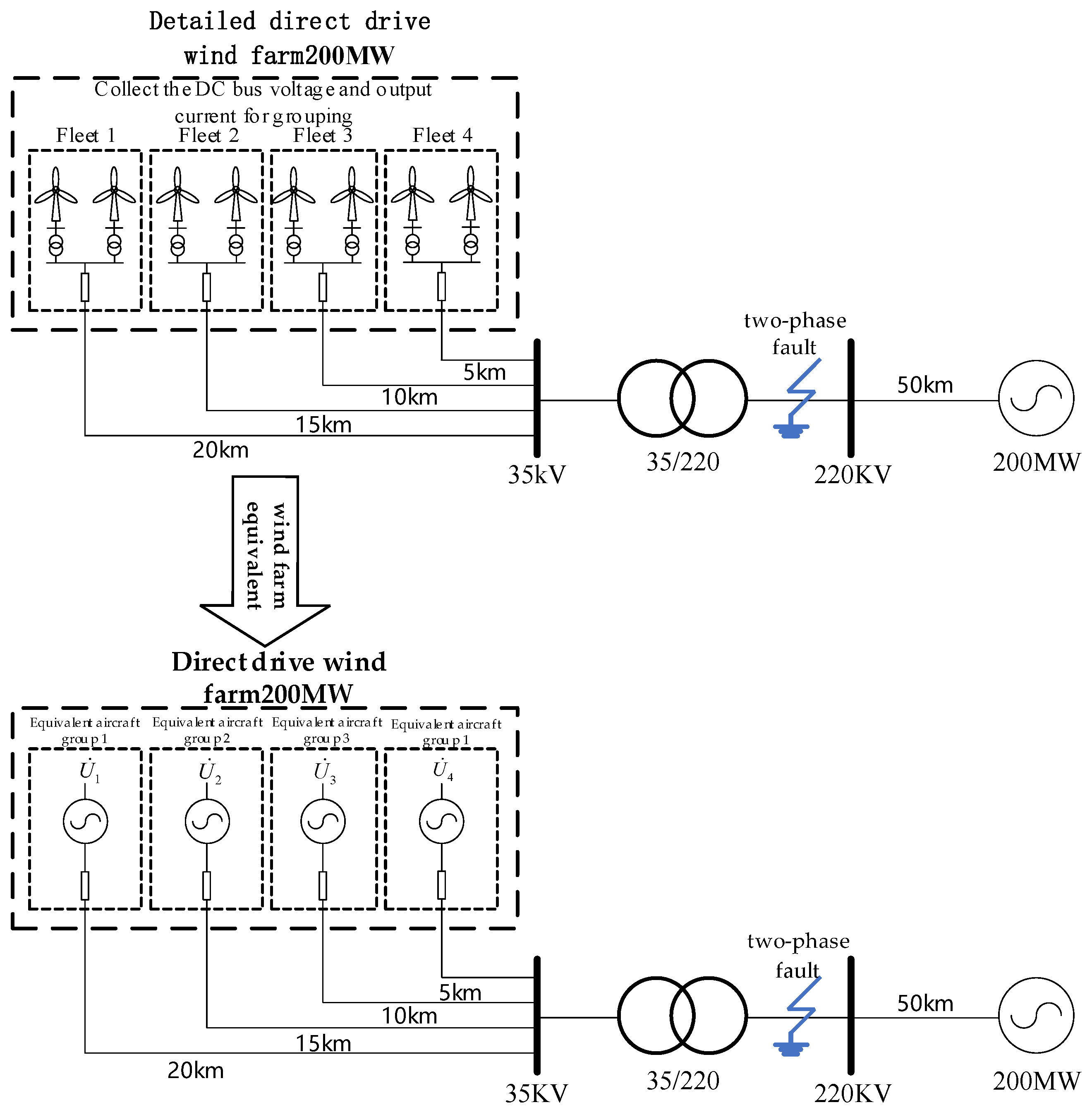
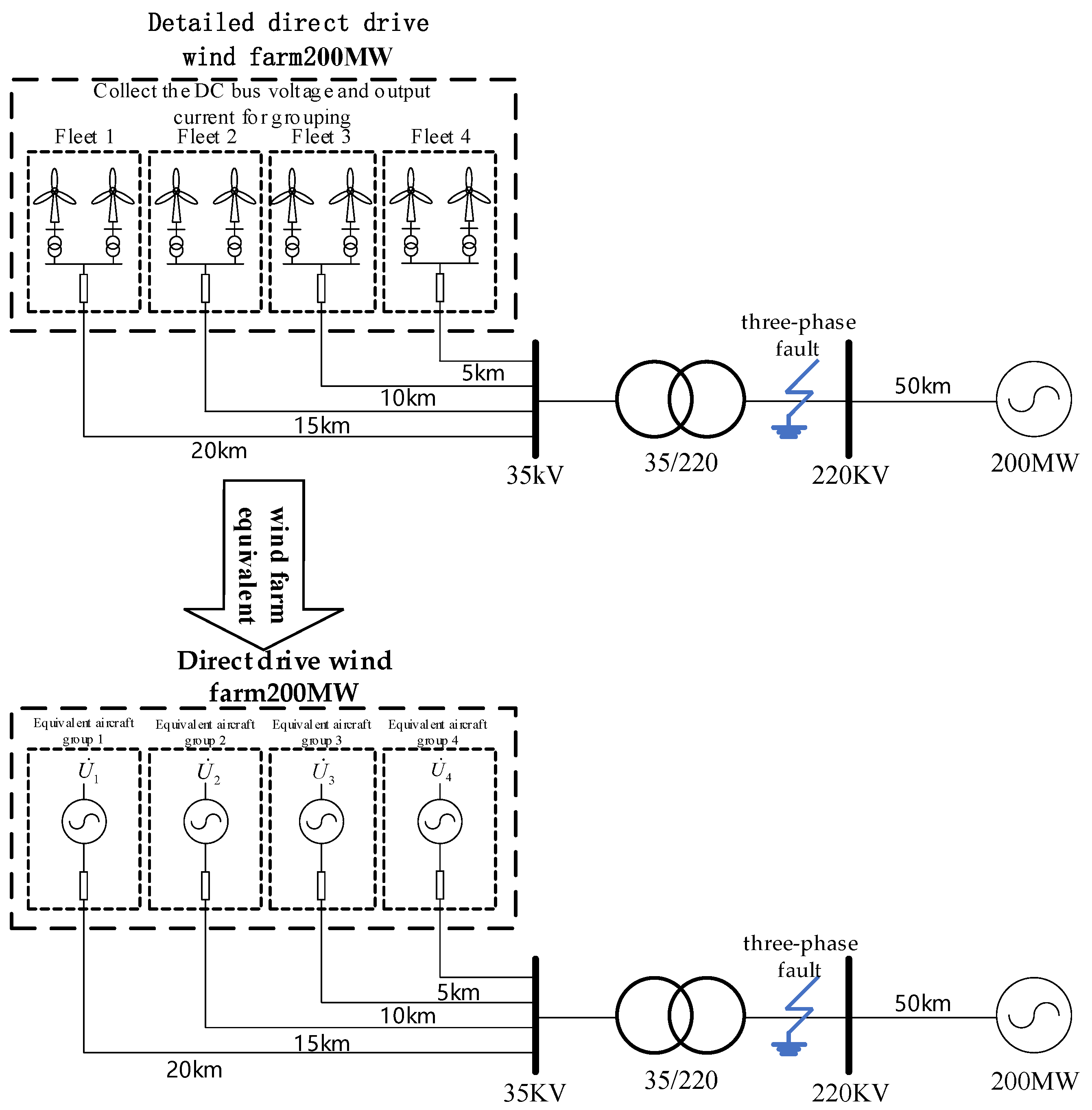
The detailed model of the wind farm with two-phase faults and its three-phase faults used in this paper and the structure and line topology of the equivalent model of the wind farm are shown in Figure 10 and Figure 11. The relevant parameters of a single wind turbine in the detailed model of the wind farm, including the PI control parameters, are provided by the State Grid Ningxia Electric Power Research Institute (SGNNEPRI) and are shown in

Table 4. Basic parameters of four types of wind turbine models inside wind farms.

	Type I Fan	Type II Fan	Type III Fan	Type IV Fan
Quantity(unit)	25	25	30	20
Rated power (MW)	2	2	2	2
Maximum output current on the network side (pu)	1.1	1.12	1.5	1.2
Operating voltage Udcmax (KV)	1.36	1.4	1.44	1.48
DC bus capacitor (mF)	1.5	2.5	3.5	4.5
Load-reducing resistor (Ω)	1.5	1.8	2.2	2.5

and

Table 5. Critical control parameters for four types of wind turbine models within wind farms.

	Type I Fan	Type II Fan	Type III Fan	Type IV Fan
Side of machine speed outer ring	0.25, 25	0.42, 25	0.55, 30	0.5, 50
Machine-side current inner ring	3, 0.01	0.5, 0.05	0.2, 0.02	0.3, 0.01
Network side reactive power outer ring	0.5, 0.75	0.15, 0.5	0.55, 0.25	2.2, 0.05
Network side voltage outer ring	0.5, 0.02	0.75, 0.05	1.5, 0.4	2.25, 0.1
Mesh side current inner ring	1, 0.01	1.53, 0.01	2.28, 0.01	1.3, 0.01

.

1.

Detailed wind farm model and equivalent fault simulation for two-phase faults;

The simulation time was set to 1.5 s, and a two-phase-to-ground short-circuit fault was applied at 1 s, with a fault duration of 0.1 s.

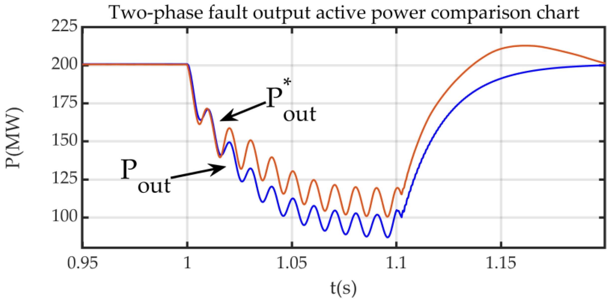
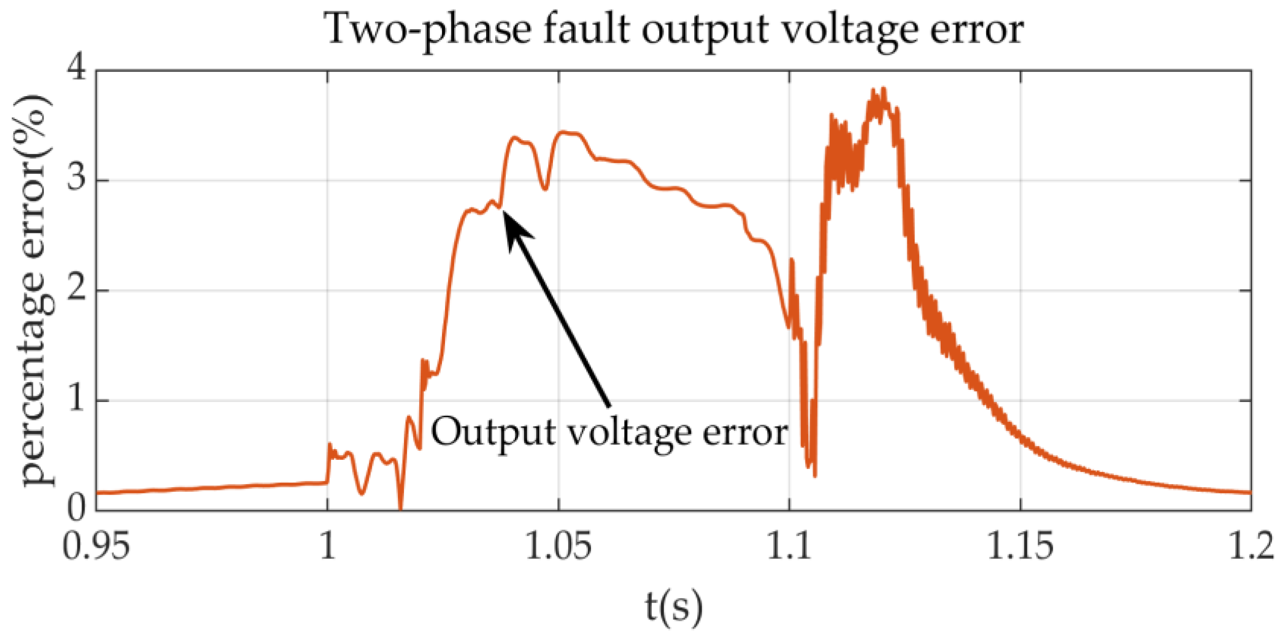
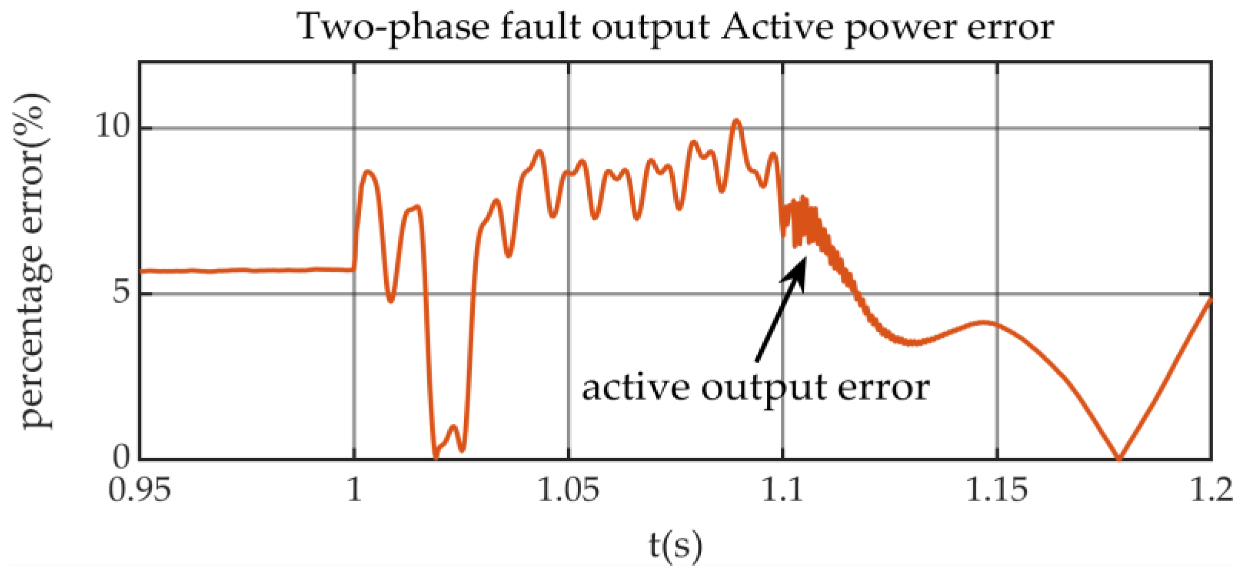
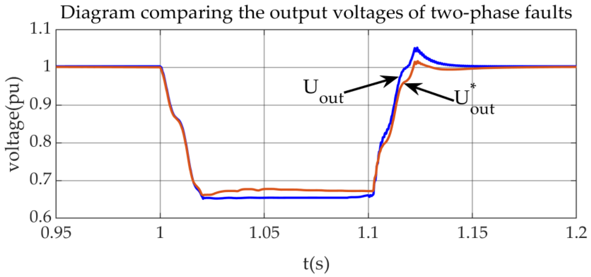
Figure 12 and Figure 13 show the waveform comparison and error analysis of the machine-side output active power between the detailed model and the equivalent model under two-phase fault conditions, while Figure 14 and Figure 15 show the waveform comparison and error analysis of the machine-side output voltage between the detailed model and the equivalent model under two-phase fault conditions. 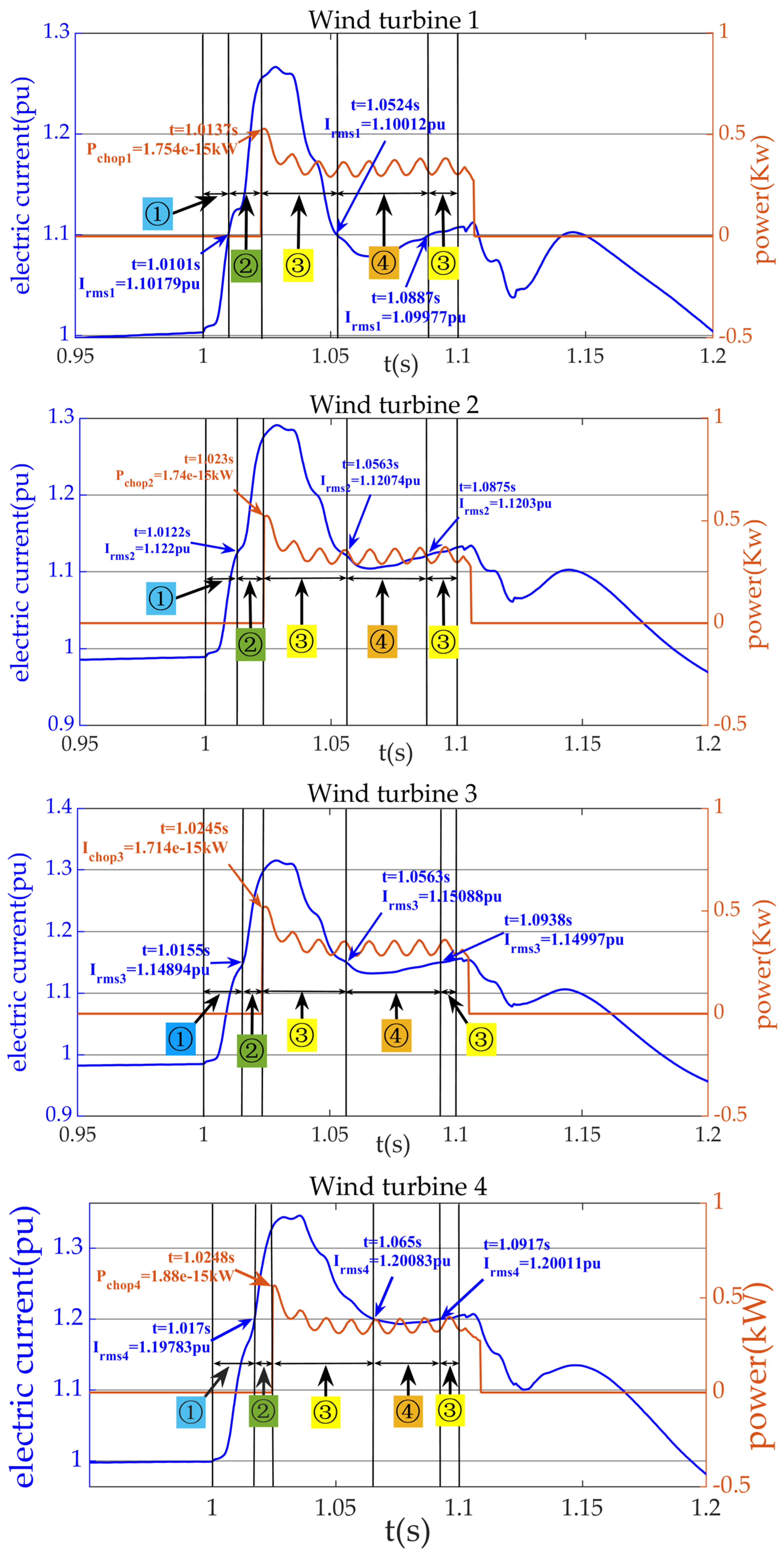In Figure 12, P_out is the output active power of the detailed wind farm model and $P_{\mathrm{out}}^{*}$ is the output active power of the equivalent wind farm; in Figure 14, U_out is the output voltage of the detailed wind farm model and $U_{\mathrm{out}}^{*}$ is the output voltage of the equivalent wind farm; and in Figure 16, I_rms is the output current of the wind turbines in the detailed wind farm and P_chop is the power consumed by the discharge resistor of the wind turbines in the detailed wind farm. It can be seen from Figure 12 and Figure 14 that after a two-phase short-circuit fault occurs in 1 s, the machine-side output voltage of the detailed wind farm model drops rapidly to 0.65 pu. At the same time, due to the influence of the control and resistance of each unit in the wind farm, the output current of each wind turbine cannot track the voltage drop rate. Therefore, the machine-side output active power of the detailed direct-drive wind farm model side output active power rapidly drops from 200 MW in the stable state to around 100 MW. Afterwards, with the grid-side converter fault ride-through control protection being engaged and the fault voltage no longer dropping, the wind farm’s machine-side output current and voltage gradually stabilize. Therefore, the machine-side output active power also temporarily stabilizes at around 100 MW stability. Soon after the disappearance of the 1.1 s two-phase fault, the detailed wind farm machine-side output voltage began to recover, and the active power began to rise from the minimum value and recover to a stable state. At the same time, by observing and comparing the equivalent model output active power and voltage, it can be clearly seen that the equivalent model active power and voltage waveforms also conform to the above change process. In addition, according to the error data of the output active power and output voltage in Figure 13 and Figure 15, it can also be intuitively concluded that within the transient period of 100 ms after a fault occurs, the maximum percentage error of the active power and output voltage of the equivalent model does not exceed 0.1,which proves the accuracy of the equivalent model designed in this paper.

Figure 16 shows the 100 ms transient region diagram of the four types of units within the wind farm fleet under a two-phase fault. The fault transient of each group of units can be divided into four regions, where ①, ②, ③, and ④ represent the fleet being in the modes: ① chopper engaged with fault ride-through control not engaged, ② chopper not engaged and fault ride-through control engaged, ③ chopper and fault ride-through control both engaged, and ④ neither chopper nor fault ride-through control engaged. It can be seen from the figure that after a two-phase fault and short circuit occurs in the wind farm, the change sequence of the modal types of each group of wind turbines during the transient process is the same, starting from the beginning of the fault: chopper and fault ride-through control not put into use—chopper is not put into use but fault ride-through control is—chopper and fault ride-through control are both put into use—chopper is put into use and fault ride-through control is not put into use. However, there is also a difference in the time of change in the modal types of each group of wind turbines in the wind farm. This is due to the different maximum output currents of the grid-side converters and the operating voltages of the protection circuits in each group of wind turbines, as well as the different distances from the fault point. The conclusion that the modal change times are different is consistent with the wind farm modelling approach envisaged in this paper.

2.

Detailed wind farm model and equivalent fault simulation under three-phase fault;

The simulation was set to last 1.5 s, with a three-phase ground fault being applied at 1 s and the fault lasting 0.1 s.

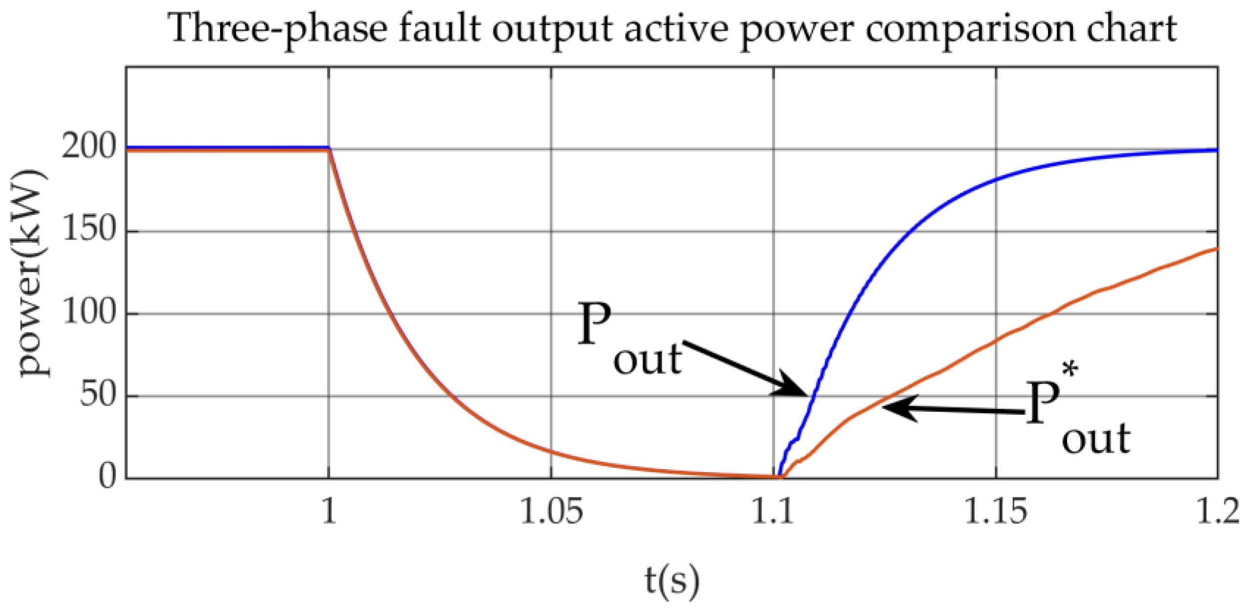
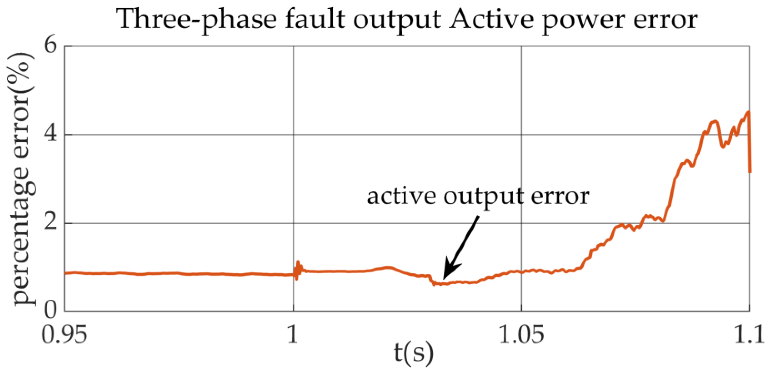
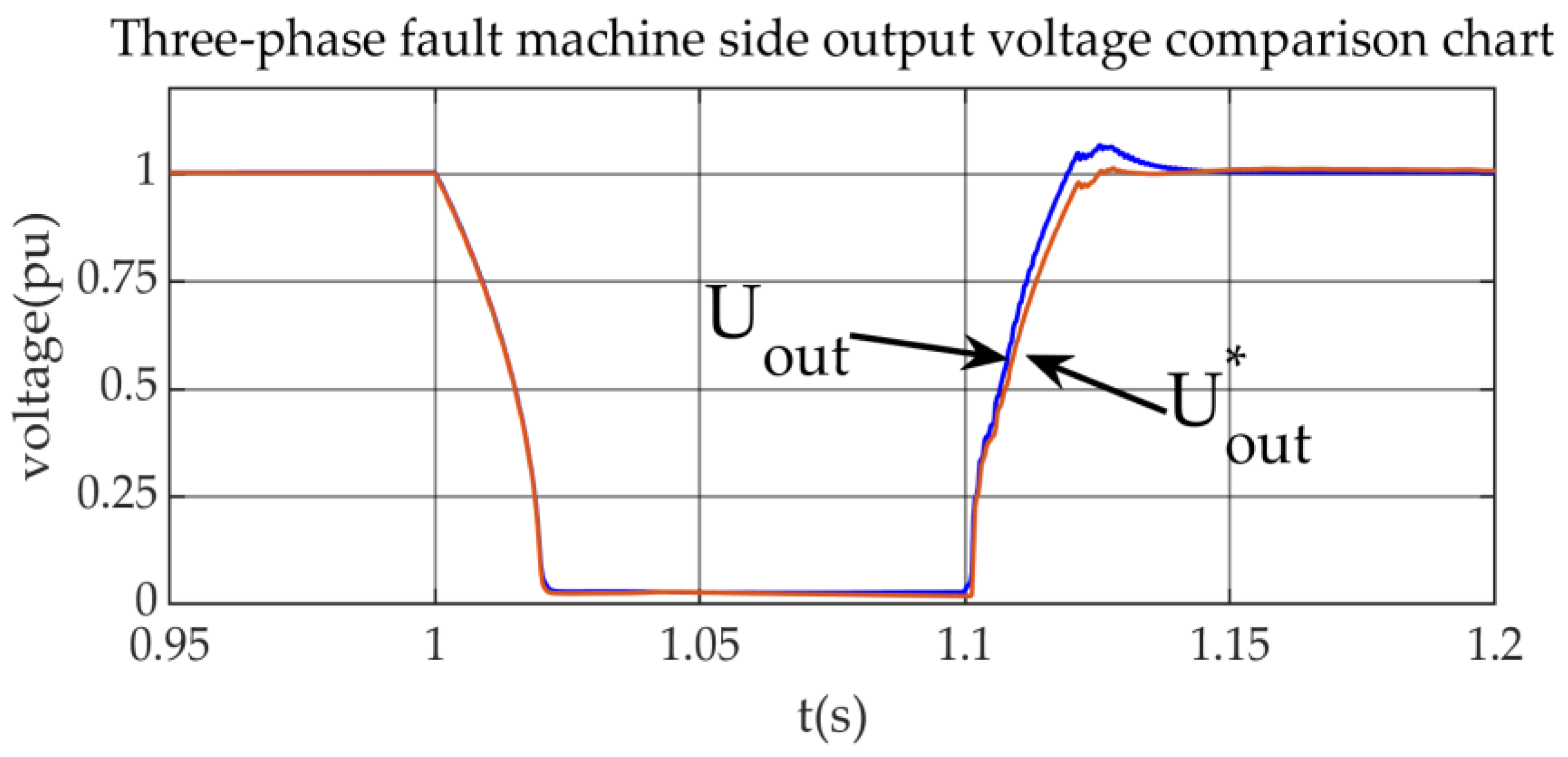
Figure 17 and Figure 18 show the waveform comparison and error analysis of the machine-side output active power between the detailed model and the equivalent model under three-phase fault conditions. Figure 19 and Figure 20 show the waveform comparison and error analysis of the machine-side output voltage between the detailed model and the equivalent model under three-phase fault conditions. It can be seen from Figure 17 and Figure 19 that after a two-phase short circuit fault occurs in 1 s, the detailed wind farm model’s machine-side output voltage drops rapidly to 0.027 pu, and the active power output of the detailed direct-drive wind farm model from the steady state of 200 MW quickly dropped to around 1.2 MW. The speed of the active power drop showed a trend of first being fast, then becoming stable, until the active power reached its lowest value at 1.1 s, at which time the active power output of the wind farm was approximately 0.45 MW.

In addition, by comparing the detailed model and equivalent model machine-side output active power and output voltage waveforms in the 100 ms transient region after a fault occurs, it can be seen that the equivalent model machine-side output active power and voltage trends are consistent with the detailed model. However, according to the error data of the output active power and voltage in Figure 18 and Figure 20, it can be concluded that during the 100 ms transient time after the fault occurs, the maximum percentage error of the active power of the equivalent model does not exceed 0.1. The active power meets the verification requirements, but the side output voltage has a maximum percentage error of 85%, and its error value cannot meet the model verification requirements. A possible reason for this result is that the voltage drop due to a three-phase fault is too large, and the detailed model output voltage value is close to 0, making the denominator too small during the calculation of the voltage error, thus causing the output voltage error to be too large during the fault transient process.

Figure 21 shows the 100 ms transient region diagram of the units within the wind farm fleet under a three-phase fault. Similar to the classification of the fleet transient region under a two-phase fault, the transient fault of each group of units in the fleet under a three-phase fault includes three modal types: ① chopper and fault ride-through control not engaged, ③ chopper and fault ride-through control engaged, and ④ chopper engaged while fault ride-through control not engaged. As can be seen from the figure, after a three-phase fault and short circuit occurs in the wind farm, the transient equivalent mode of each group lacks the mode link of chopper not engaged fault ride-through control engaged. This is because the three-phase fault voltage drop is the most serious, which causes the chopper of each group to be engaged before the fault ride-through control and the process to be more persistent. The sequence of changes in the modal types of the groups of wind turbines in a wind farm during a three-phase fault can be divided into two categories. The first category from the beginning of the fault, in order, is: chopper—both FRT control and chopper are not engaged—chopper is engaged and FRT control is not engaged—chopper and FRT control are both engaged—chopper is engaged and FRT control is not engaged—chopper and FRT control are both engaged. The second category is: chopper and FRT control are not engaged—chopper is engaged and FRT control is not engaged—chopper and FRT control are both engaged. The modal change time of each group of wind turbines differs between the two types of wind farms, with significant variations among their groups.

5. Conclusions

This paper is based on the existing fault transient model of a direct-drive wind turbine. A multi-machine grouping equivalence method is used to further upgrade to a transient multimodal equivalence modelling of the wind farm. This paper first introduces a detailed model of the wind turbine, analyzes the fault characteristics of the protection equipment and the fault ride-through control strategy during the fault ride-through process, and, based on this, the fault ride-through process of the wind turbine is segmented in multiple modes. A transient model of the wind turbine is established by simplifying and reducing the order. Finally, using the wind turbine’s own chopper and fault ride-through control protection strategy, the wind farm with complex and diverse internal fault modes is grouped, then the transient and steady-state equivalent methods were used for each group of machines using the equivalent of a single machine in the form of a controllable voltage source and current source, respectively. The equivalent model of the wind farm was verified from different perspectives using two-phase and three-phase faults of different fault levels. The results show that the equivalent model of the wind farm proposed in this paper meets the design requirements in terms of accuracy, and there has also been great progress in terms of applicability. Therefore, the transient equivalent modelling method for wind farms used in this paper is of great significance for analyzing the transient characteristics and stability of large-scale grid-connected wind farms. In particular, it can more accurately model the dynamic characteristics of wind farms with units that have different responses to faults.

6. Discussion

Based on a thorough investigation and analysis of the current mainstream equivalent methods for clustering and grouping wind farms at home and abroad, as well as the multimodal characteristics of WTGs’ own fault ride-through, combined with the advantages of the quantum particle swarm optimization algorithm, this study investigates a wind farm fault transient modelling method based on the combined grouping equivalence of WTG fault ride-through control and chopper. It proposes a new idea of using the difference in the response of WTGs’ own protection control under transient faults to form an equivalent modelling theory for complex internal wind farms.