Numerical Simulation on Aerodynamic Noise of (K)TS Control Valves in Natural Gas Transmission and Distribution Stations in Southwest China

Abstract

Fluid dynamic noise produced by eddy disturbances and friction along pipe walls poses a significant challenge in natural gas transmission and distribution stations. (K)TS control valves are widely used in natural gas transmission and distribution stations across Southwest China and are among the primary sources of noise in these facilities. In this study, a 3D geometric model of the (K)TS valve was developed, and the gas flow characteristics were simulated to analyze the gas flow field and sound field within the valve under varying pipeline flow velocities, outlet pressures, and valve openings. The results demonstrate that accurate calculations of the 3D valve model can be achieved with a grid cell size of 3.6 mm and a boundary layer set to 3. The noise-generating regions of the valve are concentrated around the throttle port, valve chamber, and valve inlet. The primary factors contributing to the aerodynamic noise include high gas flow velocity gradients, intense turbulence, rapid turbulent energy dissipation, and vortex formation and shedding within the valve. An increase in inlet flow velocity intensifies turbulence and energy dissipation inside the valve, while valve opening primarily influences the size of vortex rings in the valve chamber and throttle outlet. In contrast, outlet pressure exerts a relatively weak effect on the flow field characteristics within the valve. Under varying operating conditions, the noise directivity distribution remains consistent, exhibiting symmetrical patterns along the central axis of the flow channel and forming six-leaf or four-leaf flower shapes. As the distance from the monitoring point to the valve increases, noise propagation becomes more concentrated in the vertical direction of the valve. These findings provide a theoretical basis for understanding the mechanisms of aerodynamic noise generation within (K)TS control valves during natural gas transmission, and can also offer guidance for designing noise reduction solutions for valves.

1. Introduction

As the cleanest fossil fuel energy, natural gas is considered a good solution for reducing the levels of environmental pollution [1]. However, with the rapid development of the natural gas industry, a series of environmental pollution issues, particularly noise pollution, have become increasingly prominent. Natural gas transmission and distribution stations play important roles in the storage, dispatch, and distribution of natural gas during its transmission and distribution processes. When a natural gas transmission and distribution station regulates the pressure for measurement or distribution, the flow state of the airflow inside the pipes changes and generates eddy disturbances accompanied by friction along the pipe walls, which eventually produces fluid dynamic noise, namely, aerodynamic noise [2]. Aerodynamic noise is one of the primary types of noise in natural gas transmission and distribution stations, and its generation, propagation, and control have received increasing attention [3,4,5,6].

Early research on aerodynamic noise was dominated by theoretical analyses and experiments [7,8,9]. However, traditional experimental methods in the field of natural gas aerodynamic noise require high-precision acoustic measuring instruments and must consider the influence of environmental factors such as ambient noise, temperature, and humidity. At the same time, it is difficult to conduct high-temperature, high-pressure gas pressurization and depressurization tests, as well as tests with flammable hazardous gases (such as methane), in laboratories. Moreover, repetitive processes for optimizing design in the laboratory incur high costs and significantly reduce the speed of product design. With the development of computer technology, numerical simulations have been performed, and various turbulence calculation models have been widely used [10,11,12,13]. Relying on computer technology for numerical simulations and constructing turbulence models for natural gas noise research has become a safe and efficient approach and has received widespread attention. For example, Zhao et al. [10] used the Ffowcs Williams–Hawkings (FW-H) method to study the sound source characteristics of steam valve aerodynamic noise and found that dipole and quadrupole sources dominate different frequency bands, with experimental data and simulation results differing by less than 3%; Shi et al. [11] studied the aerodynamic noise of regulating valves using the k-epsilon model and acoustic analogy method, finding that the deviation between the simulated sound pressure level and experimental measurements was within 2%; Su et al. [7] analyzed the distribution of sound pressure levels in natural gas manifolds using FW-H and large eddy simulation (LES), and revealed that pressure pulsation is the main source of manifold noise; Han et al. [12] promoted a calculation method based on pressure valves, effectively predicting the sound power in pipelines. However, current simulation studies on valve noise mainly use steam as the simulation fluid, with relatively few studies on aerodynamic noise simulation of valves using natural gas as the flowing medium. Moreover, structural differences in various valves would affect the flow state of natural gas inside the valves, leading to changes in the distribution and propagation characteristics of aerodynamic noise.

As an important base for the natural gas chemical industry, Southwest China has rapidly developed the natural gas industry with the increasing construction of transmission pipelines and stations in recent years. Noise pollution in natural gas transmission and distribution stations has caused complaints from surrounding residents, and has therefore become a focus of widespread concern. Although there are a variety of noise sources in natural gas stations that cause various types of noise, fluid dynamic noise produced by eddy disturbances and friction along the pipe walls and equipment is the main type of noise. The (K)TS control valve is widely used in natural gas transmission and distribution station in Southwest China and is one of the main noise sources at these stations.

Therefore, in this study, the flow and sound fields of the (K)TS control valve under different operating conditions were simulated and analyzed by establishing a 3D geometric model. The objectives are (1) to establish a 3D simulation model of the (K)TS control valve and verify the accuracy of the numerical simulation method; (2) to simulate the gas flow inside the valve under different operating conditions; (3) to analyze the main factors influencing aerodynamic noise generation inside the valve; and (4) to analyze the propagation process and characteristics of aerodynamic noise inside the valve. These results provided theoretical basis for understanding the mechanism of aerodynamic noise inside (K)TS control valves during the process of natural gas transmission and offered reference for the prevention and control of noise pollution in natural gas transmission and distribution stations.

2. Theoretical Basis

2.1. Control Equations

The fluid inside the pipeline and valve obeys basic physical conservation laws. The flow control equations include the mass conservation equation, momentum conservation equation, and energy conservation equation. The mass conservation equation is expressed as follows:

$${\displaystyle \frac{\partial \rho }{\partial t}}+{\displaystyle \frac{\partial \left(\rho u\right)}{\partial x}}+{\displaystyle \frac{\partial \left(\rho v\right)}{\partial y}}+{\displaystyle \frac{\partial \left(\rho w\right)}{\partial z}}=0$$

(1)

where ρ is the density, t is time, and $u$, $v$, and $w$ are the components of the velocity vector in the x, y, and z directions, respectively. The momentum conservation equations, also known as the Navier–Stokes equations, are expressed as

$$\rho \left({\displaystyle \frac{\partial \overrightarrow{v}}{\partial t}}+\overrightarrow{v}\cdot \nabla \overrightarrow{v}\right)=-\nabla p+\mu {\nabla }^2\overrightarrow{v}+\rho \overrightarrow{g}$$

(2)

where ρ is the density, $\overrightarrow{v}$ is the fluid velocity vector, t is time, and ∇ is the Hamiltonian operator (in the Cartesian coordinate system, $\nabla ={\displaystyle \frac{\partial }{\partial x}}\overrightarrow{i}+{\displaystyle \frac{\partial }{\partial y}}\overrightarrow{j}+{\displaystyle \frac{\partial }{\partial z}}\overrightarrow{k}$), p is the fluid pressure, μ is the dynamic viscosity, ∇² is the Laplacian operator, and ∇² = ${\displaystyle \frac{{\partial }^2}{\partial x^2}}+{\displaystyle \frac{{\partial }^2}{\partial y^2}}+{\displaystyle \frac{{\partial }^2}{\partial z^2}}$, $\overrightarrow{g}$ is the vector of gravitational acceleration. For incompressible Newtonian fluids, their components in the x, y, and z directions are as follows:

$$\begin{array}{c}\rho \left({\displaystyle \frac{\partial u}{\partial t}}+u{\displaystyle \frac{\partial u}{\partial x}}+v{\displaystyle \frac{\partial u}{\partial y}}+w{\displaystyle \frac{\partial u}{\partial z}}\right)=-{\displaystyle \frac{\partial p}{\partial x}}+\mu \left({\displaystyle \frac{{\partial }^{2}u}{\partial x^2}}+{\displaystyle \frac{{\partial }^{2}u}{\partial y^2}}+{\displaystyle \frac{{\partial }^{2}u}{\partial z^2}}\right)+\rho g_x\end{array}$$

(3)

$$\begin{array}{c}\rho \left({\displaystyle \frac{\partial v}{\partial t}}+u{\displaystyle \frac{\partial v}{\partial x}}+v{\displaystyle \frac{\partial v}{\partial y}}+w{\displaystyle \frac{\partial v}{\partial z}}\right)=-{\displaystyle \frac{\partial p}{\partial y}}+\mu \left({\displaystyle \frac{{\partial }^{2}v}{\partial x^2}}+{\displaystyle \frac{{\partial }^{2}v}{\partial y^2}}+{\displaystyle \frac{{\partial }^{2}v}{\partial z^2}}\right)+\rho g_y\end{array}$$

(4)

$$\begin{array}{c}\rho \left({\displaystyle \frac{\partial w}{\partial t}}+u{\displaystyle \frac{\partial w}{\partial x}}+v{\displaystyle \frac{\partial w}{\partial y}}+w{\displaystyle \frac{\partial w}{\partial z}}\right)=-{\displaystyle \frac{\partial p}{\partial z}}+\mu \left({\displaystyle \frac{{\partial }^{2}w}{\partial x^2}}+{\displaystyle \frac{{\partial }^{2}w}{\partial y^2}}+{\displaystyle \frac{{\partial }^{2}w}{\partial z^2}}\right)+\rho g_z\end{array}$$

(5)

where u, v, and w are the components of fluid velocity in the x, y, and z directions, respectively; p is the fluid pressure; ρ is the density; μ is the dynamic viscosity; and g_x, g_y, and g_z are the components of gravitational acceleration in the x, y, z directions, respectively. The energy equation, which is the basic control equation for fluid flow and heat transfer, is expressed as

$$\rho c_p\left({\displaystyle \frac{\partial T}{\partial t}}+\overrightarrow{v}\cdot \nabla T\right)=\nabla \left(k\cdot \nabla T\right)+\mathsf{\Phi }+S_h$$

(6)

where ρ is the density, $c_p$ is the specific heat capacity at constant pressure, T is temperature, $\overrightarrow{v}$ is the fluid velocity vector, and ∇ is the Hamiltonian operator (in the Cartesian coordinate system, $\nabla ={\displaystyle \frac{\partial }{\partial x}}\overrightarrow{i}+{\displaystyle \frac{\partial }{\partial y}}\overrightarrow{j}+{\displaystyle \frac{\partial }{\partial z}}\overrightarrow{k}$), k is the thermal transfer coefficient of the fluid, and Φ is the internal heat source of the fluid and the part that the fluid mechanical energy converted into heat energy due to viscous action, abbreviated as the viscous dissipation term; $S_h$ is the heat source term, indicating the part that is externally heated or cooled.

2.2. Turbulence Model

The Reynolds-averaged Navier–Stokes (RANS) method was used in the turbulence numerical simulation in this study. The time-averaged Reynolds equation is expressed as follows [14]:

$${\displaystyle \frac{\partial }{\partial t}}\left(\rho u_i\right)+{\displaystyle \frac{\partial }{\partial x_j}}\left(\rho u_i{u}_j\right)={\displaystyle \frac{\partial p}{\partial x_i}}+{\displaystyle \frac{\partial }{\partial x_j}}\left(\mu {\displaystyle \frac{\partial u_i}{\partial x_j}}-\rho \overline{u_{i^{\prime }}{u}_{j^{\prime }}}\right)+S_i$$

(7)

where $\rho$ is the density of the fluid (mass per unit volume); $u_i$ is the velocity components in the i-th direction. The index i can correspond to the directions x, y, or z in a three-dimensional space. $\rho u_i{u}_j$ represents the convective acceleration of the fluid, with u_i being the velocity in the i-direction, and u_j in the j-direction. The indices i and j cover the directions in space (e.g., i = x, y, z). p is the pressure within the fluid, $x_i$ is the spatial coordinates in the i-direction, μ is the dynamic viscosity of the fluid, and $S_i$ is likely a source term, representing external forces or influences acting on the fluid. In the closed equation system, the following assumptions are made: introducing turbulent viscosity, expressing the turbulent stress as a function of turbulent viscosity, and establishing a relationship between the Reynolds stress term (turbulent pulsation valve) and the mean velocity gradient (time-averaged valve), that is:

$$-\rho \overline{u_{i^{\prime }}{u}_{j^{\prime }}}={\mu }_t\left({\displaystyle \frac{\partial u_i}{\partial x_j}}+{\displaystyle \frac{\partial u_j}{\partial x_i}}\right)-{\displaystyle \frac{2}{3}}\left(\rho k+{\mu }_t{\displaystyle \frac{\partial u_i}{\partial x_i}}\right){\delta }_{\mathrm{ij}}$$

(8)

where $-\rho \overline{u_{i^{\prime }}{u}_{j^{\prime }}}$ represents the Reynolds stress tensor, and the negative sign comes from the convention used in turbulence modeling; ${\mu }_t$ is the turbulent viscosity, which is a function of spatial coordinates and depends on the flow state; $\left({\displaystyle \frac{\partial u_i}{\partial x_j}}+{\displaystyle \frac{\partial u_j}{\partial x_i}}\right)$ is the rate of strain tensor, representing the mean velocity gradient symmetrized to reflect the effect of turbulence on momentum transfer; $u_i$ is the time-averaged velocity, k is the turbulent kinetic energy (TKE), ${\delta }_{ij}$ is the Kronecker function symbol (when $i=j$, ${\delta }_{ij}=1$; when $i\ne j$, ${\delta }_{ij}=0$), and k is the turbulent kinetic energy, calculated as

$$\begin{array}{c}k={\displaystyle \frac{\overline{u_{i^{\prime }}{u}_{j^{\prime }}}}{2}}\end{array}$$

(9)

where k is turbulent kinetic energy (TKE), which quantifies the intensity of turbulence in a fluid flow; $u_{i^{\prime }} \mathrm{and} u_{j^{\prime }}$ are the fluctuating velocity components in the i-th and j-th directions; the prime (′) indicates that these are deviations from the mean velocity.

2.3. Broadband Noise Model

Using the data of velocity field, turbulence quantities, and dissipation rate obtained from the Reynolds-averaged equations, the Proudman equation is used to calculate the sound power generated by the flow [15]:

$$P_A=\alpha {\rho }_0\left({\displaystyle \frac{u^3}{l}}\right){\displaystyle \frac{u^5}{a_0^5}}$$

(10)

where P_A is the sound power, W/m³; α is a constant coefficient, which may be related to material properties or experimental conditions; ${\rho }_0$ represents the density of the fluid or medium; u is the turbulent velocity, m/s; l is turbulent characteristic length, m; $a_0$ is the sound velocity, m/s.

Exponents like $u^3$ and $u^5$ indicate a relationship between the velocity and some physical effects, where the velocity may be raised to the power of three and five in relation to specific scales or phenomena. In Fluent, the sound power is expressed as the sound power level using the following formula:

$$L_P=10\log \left({\displaystyle \frac{P_A}{P_{ref}}}\right)$$

(11)

where $L_P$ is the sound power level, measured in decibels (dB); $P_A$ is the actual sound power being measured; P_ref is the reference sound power, typically 10⁻¹² W/m².

2.4. FW-H Acoustic Analogy Method

The FW-H equation adopts the general form of Lighthill’s acoustic analogy to predict the sound generated by equivalent sound sources. The time-accurate solution of flow field variables are obtained from transient Reynolds-averaged equations, and surface integral methods are used to calculate the acoustic signals at monitoring points. The FW-H equation can be written as follows [16]:

$$\begin{array}{c}{\displaystyle \frac{1}{a_0^2}}{\displaystyle \frac{{\partial }^2{p}^{\prime }}{\partial t^2}}-{\nabla }^2{p}^{\prime }={\displaystyle \frac{{\partial }^2}{\partial x_i\partial x_j}}\left\{T_{ij}H\left(f\right)\right\}-{\displaystyle \frac{\partial }{\partial x_i}}\left\{\left[P_{ij}{n}_j+\rho u_i\left(u_n-v_n\right)\right]\delta \left(f\right)\right\}\\ +{\displaystyle \frac{\partial }{\partial t}}\left\{\left[{\rho }_0{v}_n+\rho \left(u_n-v_n\right)\right]\delta \left(f\right)\right\}\end{array}$$

(12)

where $p^{\prime }$ is the far-field sound pressure in Pa, $a_0$ is local sound velocity in m/s, t is the time; $x_i \mathrm{and} x_j$ are the spatial coordinates, typically representing the position in space. $T_{ij}$ is stress or tensor term, potentially relating to the forces or stresses acting on the medium; $H\left(f\right)$ is function dependent on frequency; $P_{ij}$ is pressure-related term; $u_i$ is the fluid velocity component in m/s; $u_n$ is the specific velocity term; $v_n$ is the surface velocity component in m/s, $T_{ij}$ is the Lighthill stress tensor in Pa, δ(f) is the Dirac delta function, and H(f) is the Heaviside function.

$$T_{ij}=\rho u_i{u}_j+P_{ij}-a_0^2\left(\rho -{\rho }_0\right){\delta }_{ij}$$

(13)

where ${ T}_{ij}$ is the stress tensor, representing the force transmission in the medium; $\rho$ is the density, indicating the mass density of the medium; $u_i{u}_j$ represent the velocity in the i and j directions. $P_{ij}$ is the stress tensor, ${\delta }_{ij}$ is the Kronecker symbol, $a_0^2$ is the speed of sound in the medium, ${\rho }_0$ is the far-field fluid density (kg/m³), and ${\delta }_{\mathrm{ij}}$ is the Kronecker delta. The time-domain signal at the monitoring point is transformed into the frequency-domain signal using the fast Fourier transform (FFT):

$$\begin{array}{c}p\left(f\right)={\displaystyle \frac{1}{2\pi }}{\int }_{-\infty }^{+\infty }p\left(t\right)e^{itf}dt\end{array}$$

(14)

where p(f) is the Fourier transform of the function p(t), where f is the frequency variable and p(t) is the original function in the time domain. $e^{itf}$ is the complex exponential factor, which represents oscillations at frequency $f$ and is used to decompose the time-domain signal into its frequency components. t is the time variable in the time-domain function p(t). $f$ is the frequency variable in the frequency-domain representation; ${\displaystyle \frac{1}{2\pi }}$ is a normalization factor to ensure that the Fourier transform is unitary and preserves the energy of the signal.

3. Geometric Model Establishment

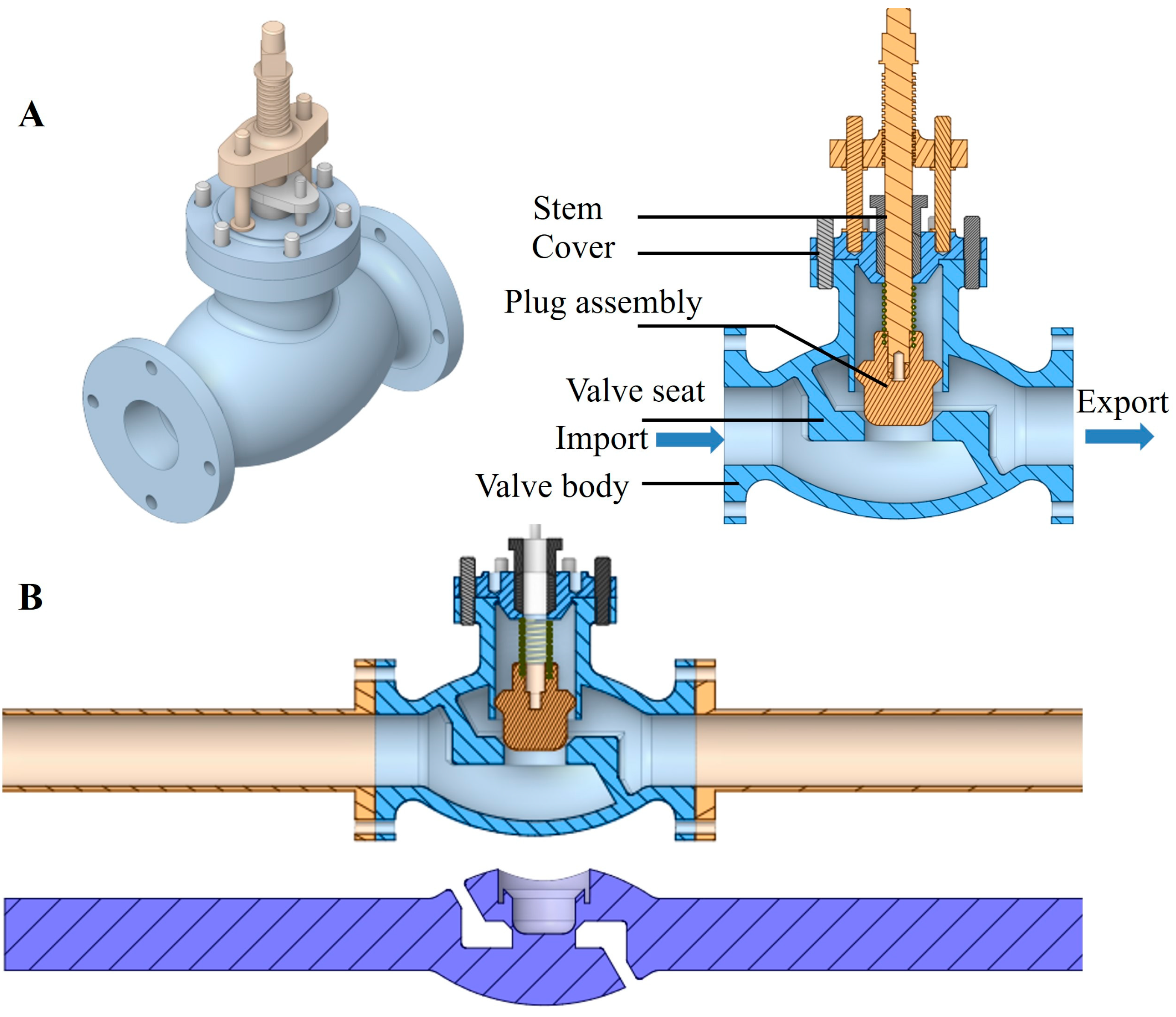
3.1. Establishment of the Geometric Model

The (K)TS control valve mainly consists of the main valve body, piston, valve seat, chamber bottom, chamber cover, and signal tube. To avoid the low work efficiency caused by the exponential increase in grid quantity, the initial model of the three-dimensional valve fluid domain was constructed by ignoring components such as the sealing ring, balancer, and signal tube, while retaining the features of the valve fluid passage based on the actual dimensions [17], as shown in Figure 1A. Some technical parameters of (K)TS control valve are listed in

Table 1. Technical parameters of (K)TS control valve.

Parameter	Value
Nominal diameter	80 mm
Nominal pressure grade	6.3 MPa
Valve body material	WCB
Valve cover material	Forged steel
Piston and valve seat materials	S30408 (Stainless steel)

. Additionally, the inlet and outlet sections of the valve were both sufficiently extended to ensure fluid flow through the valve and collect more accurate flow field data. The flow channel was extracted before the simulation analysis, and the fluid computational domain was modeled, as shown in Figure 1B.

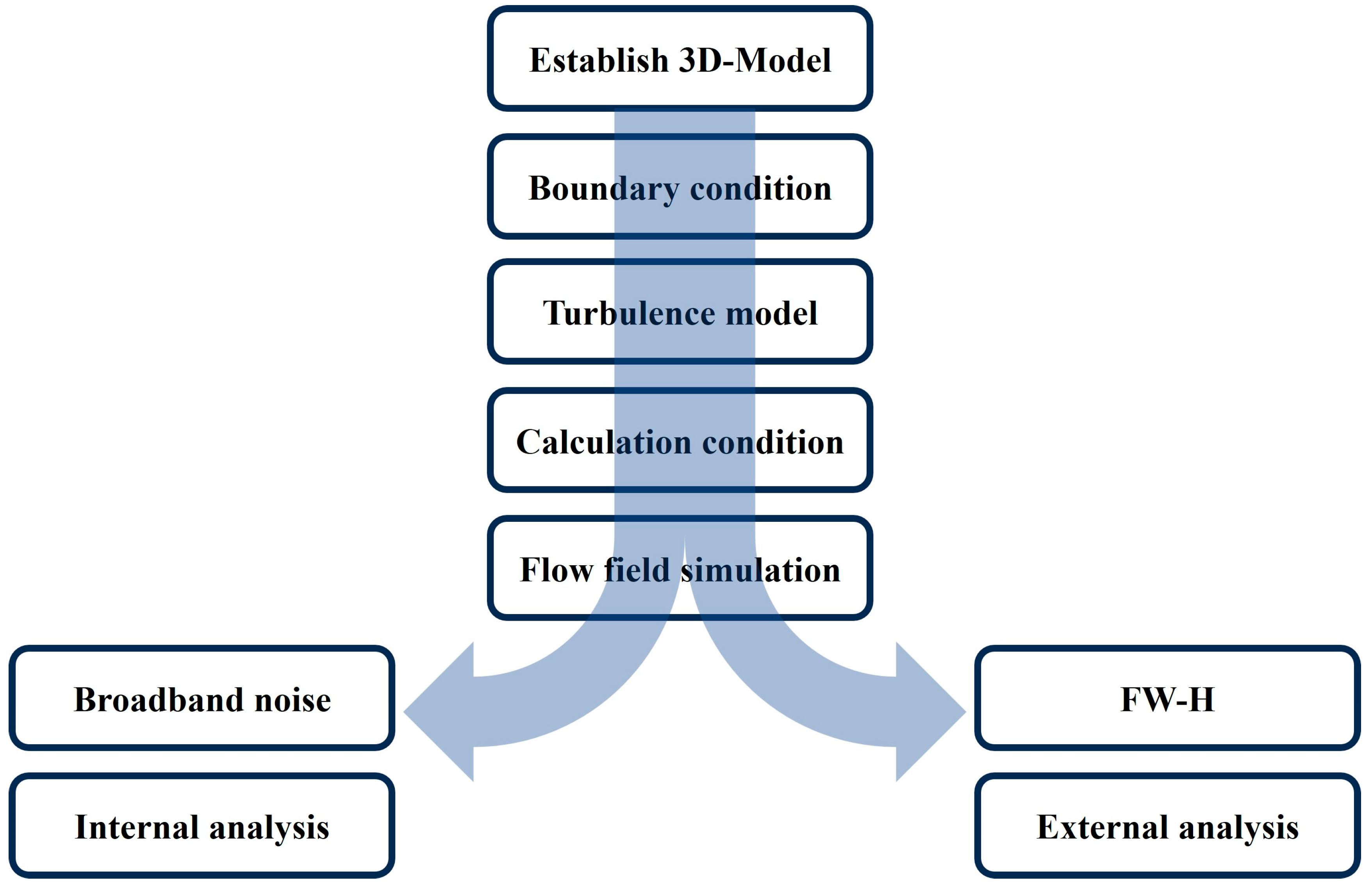
3.2. Simulation Method Settings

To conduct a simulation analysis of the aerodynamic noise flow field inside the valve, the boundary conditions for the simulation must be set. Referring to the methods of Hou et al. [18,19], the main boundary conditions for the valve in this study are set as follows: the inlet boundary is set as the velocity inlet, the pipeline flow velocity is controlled by the inlet boundary, the outlet boundary is set as the pressure outlet, and the pipeline pressure is controlled by the outlet boundary. The flow medium is natural gas (CH₄) with a density of 0.58 kg/m³ and a dynamic viscosity of 1.087 × 10⁻⁵ kg/(m·s). The total temperature was set to 297 K using adiabatic walls. The simulation calculations were performed using the computational fluid dynamics software ANSYS FLUENT (2022R2), focusing solely on the internal flow characteristics. The Realizable k-epsilon model was used as the turbulence model, and a standard wall function treatment was used near the wall surface. According to the pressure–velocity coupling scheme, the gradient was based on the least-squares method of the unit body, and the pressure and momentum were solved using the second-order upwind scheme, while the turbulent kinetic energy and turbulent dissipation rate were solved using the first-order upwind scheme. The simulation calculation process is illustrated in Figure 2.

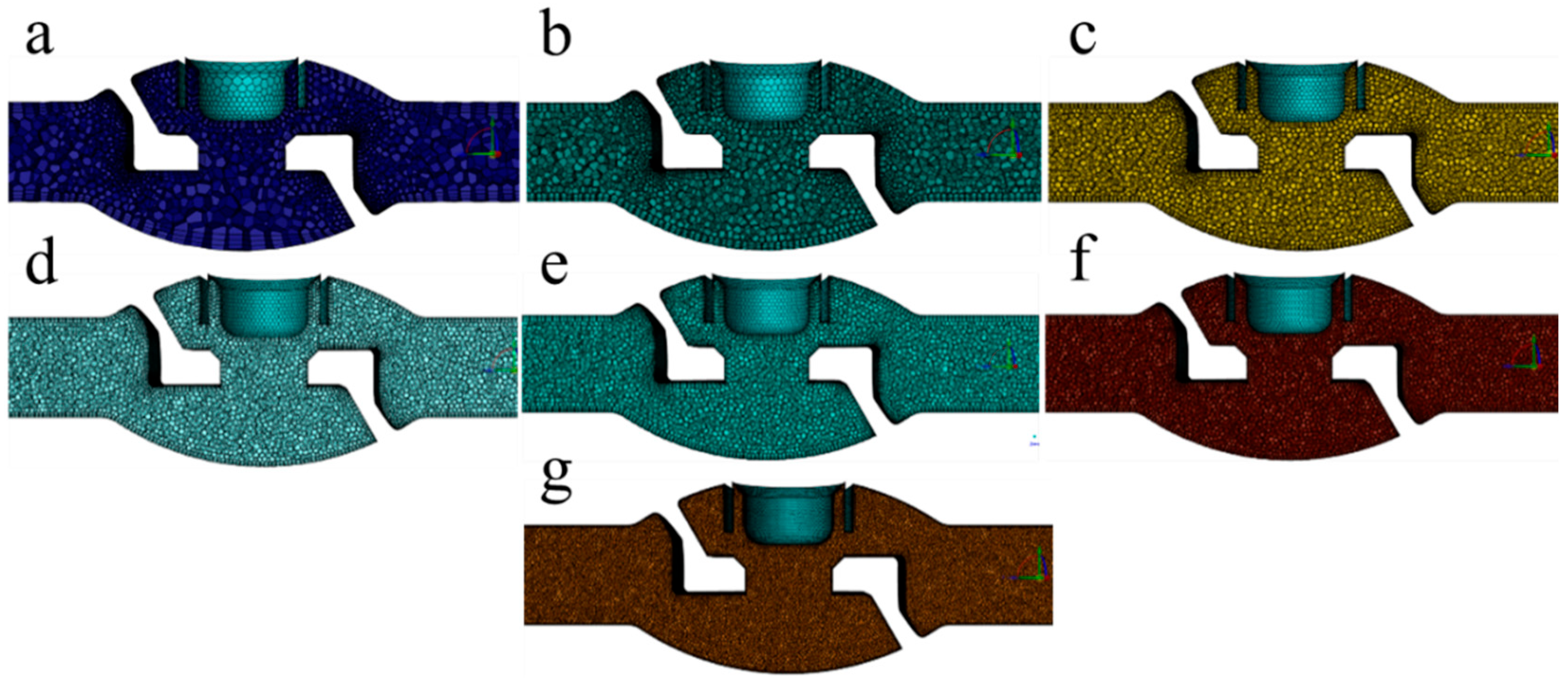
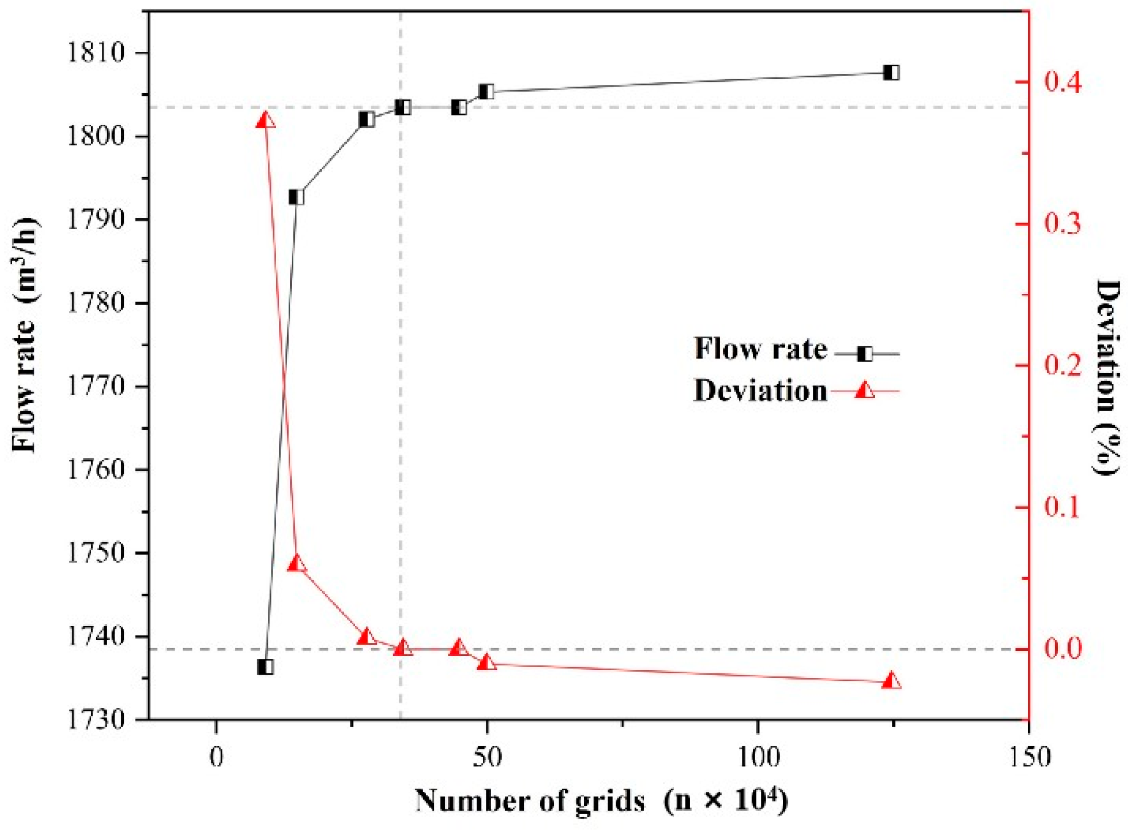
3.3. Grid Independence Verification

The accuracy of the grid affects the simulation calculation efficiency and the accuracy of the results. Therefore, before the formal calculation, to eliminate errors caused by the grid, the same boundary conditions and equipment environment were used, and the unit size was adjusted to verify the independence of the seven different sets of grids [20,21]. In this study, the grid configurations for each group are listed in

Table 2. Grid configuration for relevant verification.

No.	Maximum Unit Size (m)	Boundary Layers (n)	Number of Grids	Minimum Orthogonal Mass
1	0.0400	3	9 × 104	0.21
2	0.0060	3	1.4 × 105	0.21
3	0.0040	3	2.8 × 105	0.21
4	0.0036	3	3.4 × 105	0.20
5	0.0036	5	4.4 × 105	0.21
6	0.0030	3	5.0 × 105	0.20
7	0.0020	3	1.2 × 106	0.20

, and the polyhedral grids are shown in Figure 3. For convenience of comparison, the volumetric flow rate was used as the evaluation parameter, and the flow rate deviation of other grids was calculated based on the flow rate data of grid 4 (Q₀), with the following deviation formula:

$$\mathrm{Deviation}={\displaystyle \frac{Q_0-Q_1}{Q_0}}$$

(15)

The variation in the flow rate and the calculated deviation with the number of grids are shown in Figure 4. The flow rate calculated by the fine grid was significantly higher than that calculated by the coarse grid, and the flow rate tended to stabilize as the grid was refined. When the number of grids is less than 3.4 × 10⁵, the volumetric flow rate continues to increase with the increase in grid quantity. When the number of grids exceeded 3.4 × 10⁵, there was no significant change in the volumetric flow rate (less than 0.2%), and the number of grids had a relatively small effect on the calculation results, while the calculation efficiency decreased significantly. Therefore, in this study, a grid cell size of 3.6 mm and a boundary layer of 3 can ensure calculation accuracy to meet the requirements of grid independence verification.

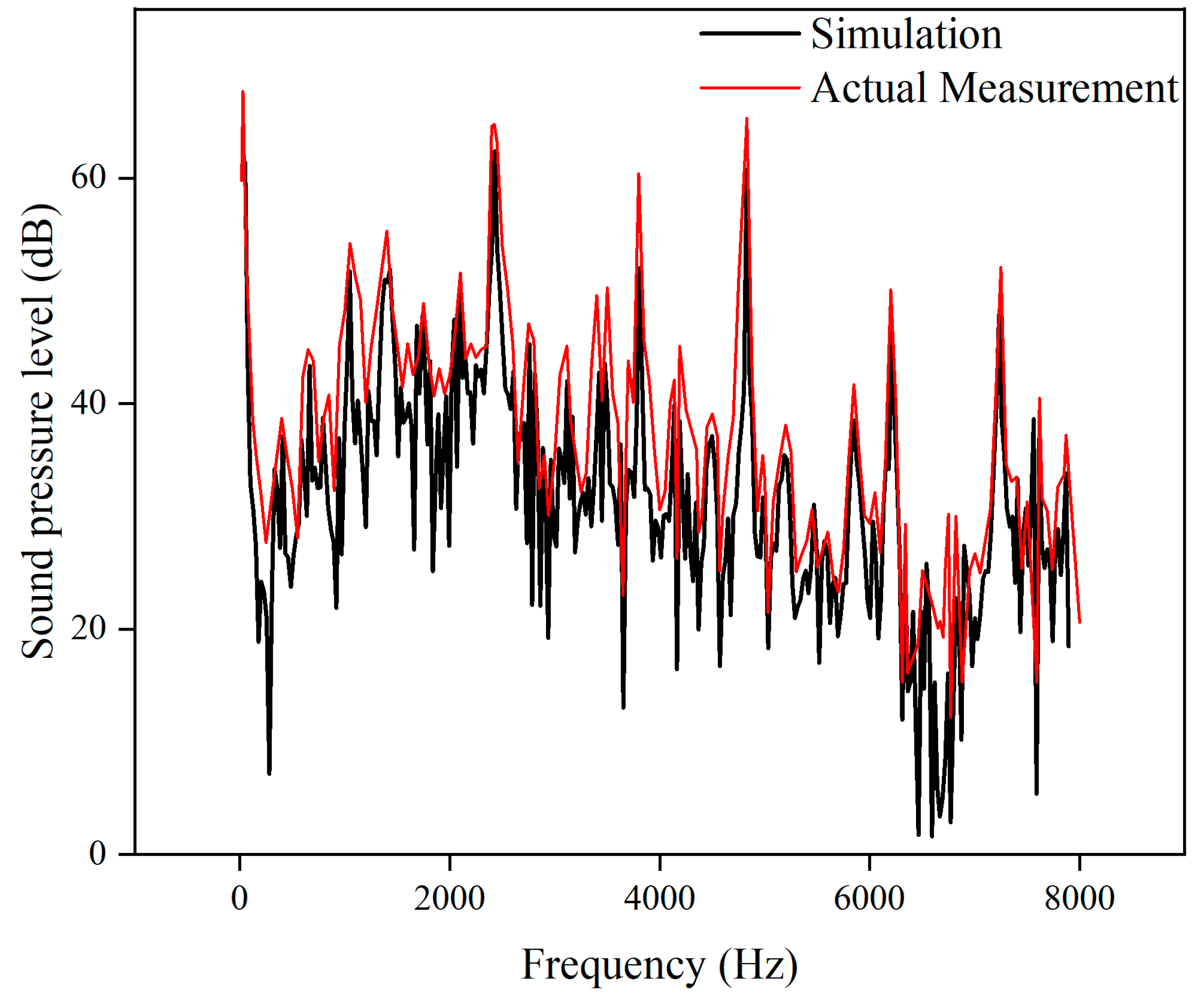
3.4. Model Validation

The feasibility of the numerical simulation method can be verified by comparing the numerical calculation results with actual monitoring results. In this study, frequency spectrum monitoring of the noise generated by the (K)TS valve under operating conditions at a newly built natural gas transmission and distribution station in Southwest China was conducted on 29 October 2023. This natural gas transmission and distribution station is located in a remote area where background noise can be almost ignored. The octave band sound pressure levels were recorded at a distance of 1 m from the valve. Using the calculation method of this study, the noise sound pressure levels at a distance of 1 m from the valve were also calculated under the same operating conditions as in the actual monitoring. It can be observed that the calculation results agree well with the actual monitoring results (Figure 5). The results show the same downward trend as the frequency increases, and the noise from this valve is broadband noise dominated by low- and mid-frequencies. The relative error of the SPL between the simulation results and actual measurement results at a distance of 1 m from the valve was less than 6%. Overall, the calculated frequency spectrum curves are similar to the measured noise spectrum curves, which indicates that this simulation method is effective and can serve as a basis for studying the noise characteristics and noise reduction analysis of the (K)TS valve.

4. Results and Analysis

To analyze the effects of different operating parameters (velocity of flow, outlet pressure, and valve opening) on the gas flow field and sound field, the pressure and velocity distribution, vortex structure, turbulence kinetic energy, turbulence dissipation rate, sound power level, time-domain fluctuation distribution of sound pressure generated with different inlet velocities ranging from 6 to 15 m/s, outlet pressure ranging from 1.6 to 2.8 MPa, and valve opening ranging from 40% to 100% were simulated, respectively. The different parameters under variable operating conditions are shown in

Table 3. Different parameters under variable operating conditions.

Parameters	Inlet Velocities v (m/s)	Outlet Pressure P (Pa)	Valve Opening Vo (%)
Value	6, 9 *, 12, 15	1.6, 2.0 *, 2.4, 2.8	40, 60, 80, 100 *

Note: * represents the value when the parameter remains unchanged.

. Unless otherwise specified, all cases in this study were simulated with one parameter changing while the other two parameters remained unchanged.

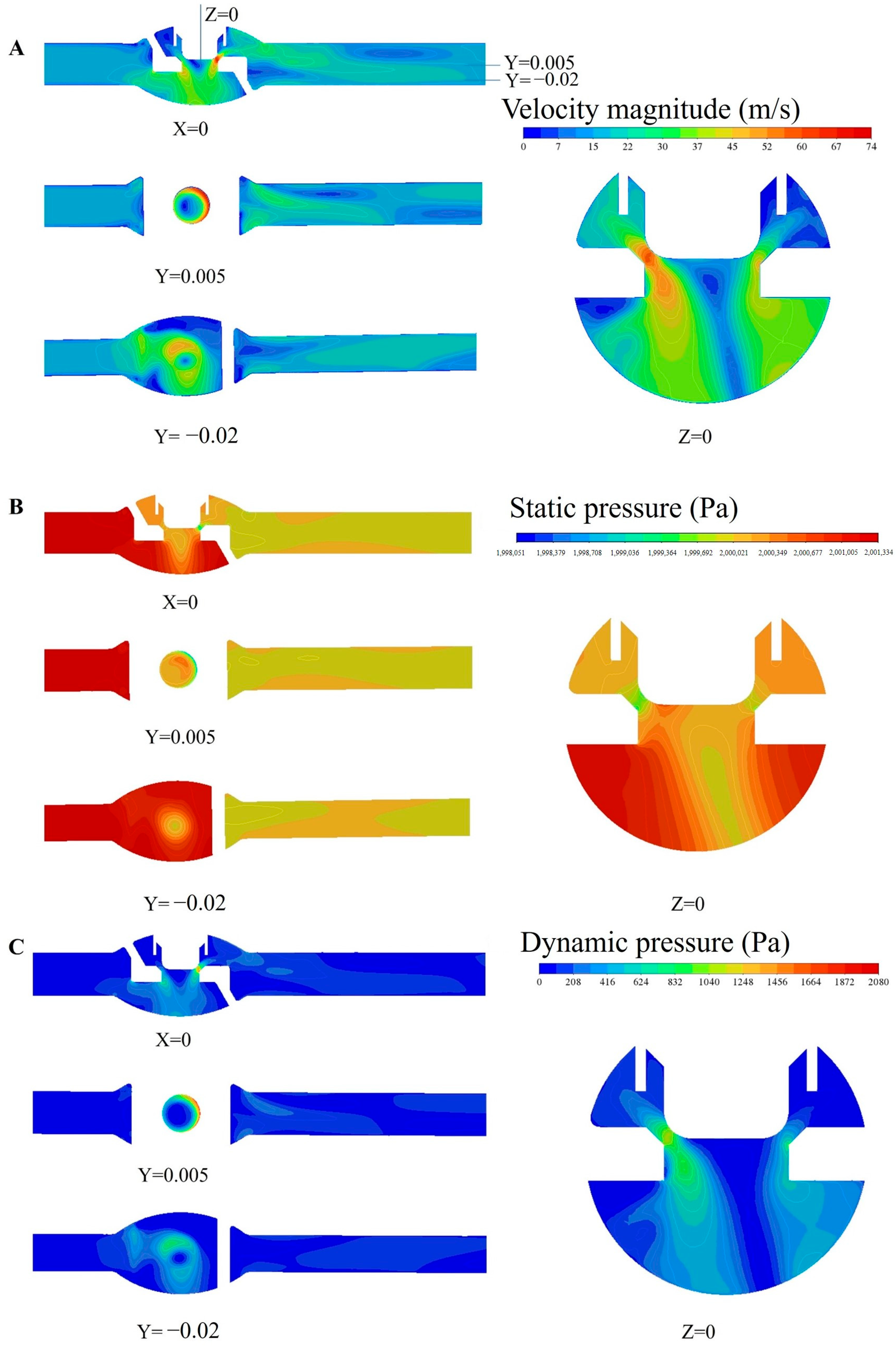
4.1. Flow Field Simulation Calculation

According to the on-site research results, the flow field characteristics of aerodynamic noise generated by the internal flow field of the (K)TS valve were studied under the working conditions of a valve opening of 60%, a pipeline flow velocity of 15 m/s, and a pipeline pressure of 2 MPa. The simulation results of the internal flow field characteristics of the valve and the velocity distributions of the different sections in the flow channel are shown in Figure 6A. Here, X = 0 represents the symmetry plane of the flow channel, with relative positions Y = −0.02, Y = 0.005, and Z = 0. The results indicate that when gas enters the valve body at a relatively low velocity, the reduction in the cross-sectional area of the flow channel owing to the contraction of the inlet pipeline increases the gas velocity, and the gas attaches to the valve wall, causing a reduction in velocity. When the simulated gas reached the lower part of the valve chamber, it underwent rotational mixing, passed through the throttle port, and collided with the bottom of the valve plug, altering the gas flow direction to move along the columnar surface of the valve plug towards the outlet. This process significantly decreases the near-wall gas velocity at the bottom of the valve plug. Owing to the sharp reduction in the cross-sectional area, the gas velocity showed a significant gradient and gradually reached its maximum when the simulated airflow passed through the throttling outlet. Finally, most of the gas reached the tail of the valve outlet, where the flow velocity decreased rapidly and formed a wake region. Additionally, a portion of the airflow can reach the upper chamber of the valve, where the flow velocity slows down, forming a low-speed zone and generating backflow. The simulation results of the static and dynamic pressure distributions on various sections of the flow channel are shown in Figure 6B and 6C, respectively. The results reveal that the dynamic pressure is higher and the static pressure is lower at the throttle port of the valve. This may be due to the fact that when natural gas flows inside the valve and encounters channel contraction, a portion of the static pressure is converted into dynamic pressure to meet the pressure required for fluid acceleration [19]. Compared to the inlet pressure, the static pressure decreases during the flow process by overcoming resistance and converting it to dynamic pressure. In areas with large corners, especially around the valve plug, the relatively dense isobaric lines indicate significant pressure variations and large pressure gradients, leading to complex separated and vortex flows.

The vortex structure generated by the gas fluid inside the valve was identified using the Q criterion, as shown in Figure 7A. The results indicated that the vortex structures were primarily concentrated at the valve inlet, valve chamber, and throttle outlet. Vortex structures are key components of turbulence and play crucial roles in fluid motion and energy conversion. When gas flows through the valve inlet and the upper part of the valve chamber, the fluid is affected by the wall surface and forms spiral vortices, but it can still maintain its own fluid structure and motion to a certain extent. As the gas reaches the lower part of the valve chamber, the vortex structures bend and twist, thereby affecting the rotation and mixing processes of the gas flow. When the gas exits the valve, the vortex structures elongate along the flow lines and rotate to form a strip vortex, which plays an important role in the mixing and transportation of gas flow. The formation of vortices indicates that the gas flow is unstable when passing through these positions. The energy in the turbulence is transferred through vortices of varying sizes until it reaches a sufficiently small vortex structure, where the energy is converted into other forms and dissipated. The turbulent kinetic energy and dissipation rate inside the valve are shown in Figure 7B. The results show that the turbulence at the center of the valve chamber has higher energy, suggesting intense turbulent motion and high fluid pulsation velocities. The areas with high turbulent dissipation rates were located near the corners of the throttle window and at the throttle outlet, indicating a rapid energy dissipation rate. Therefore, the complex gas flow inside the valve channel can generate significant rotations and vortices. The shedding of vortices can cause fluid pulsations and exciting noise that propagate through the fluid, which can be detected by monitoring equipment or the human ear. Therefore, stabilizing the internal flow state of the valve may be an important approach for reducing noise in natural gas transmission and distribution stations.

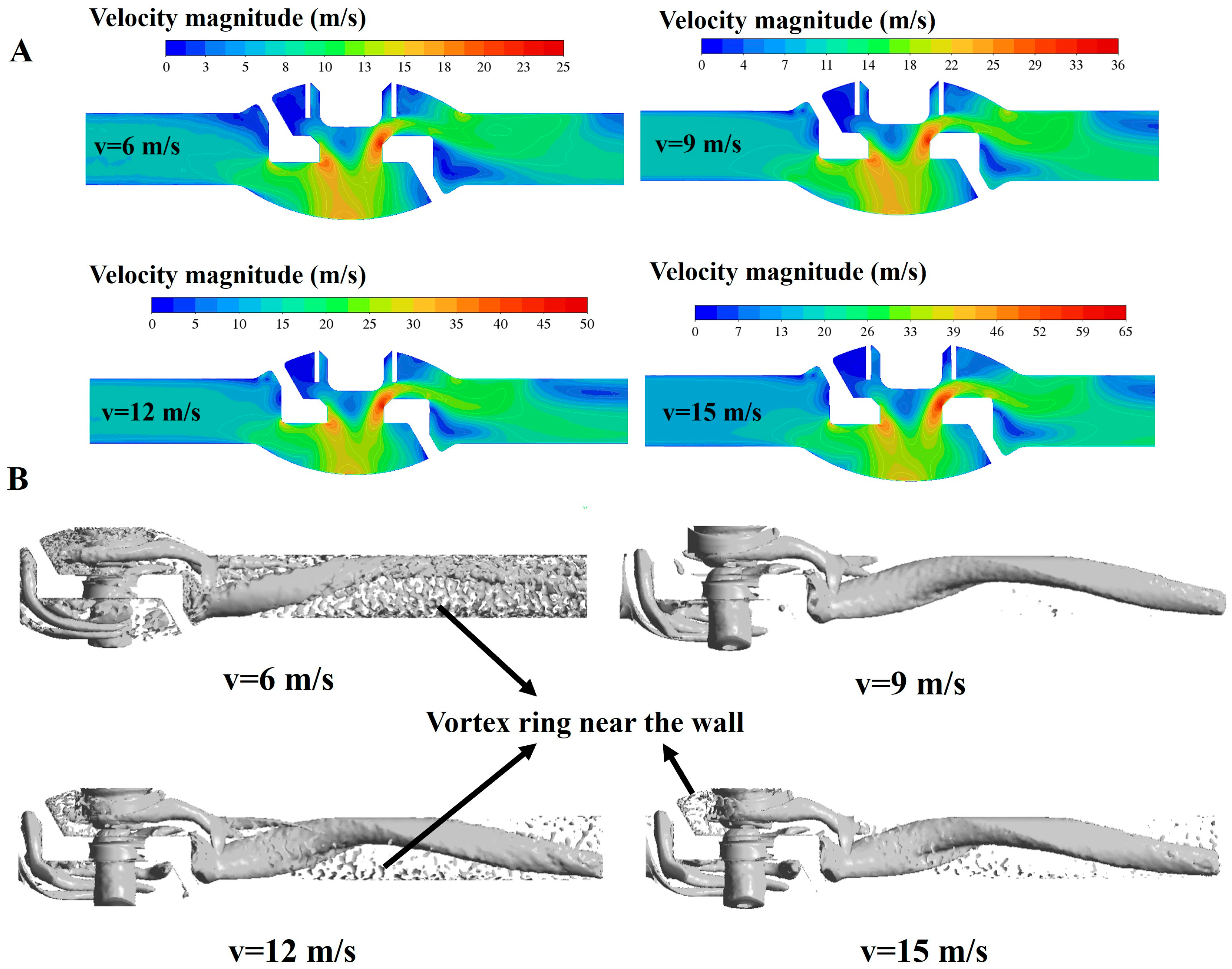
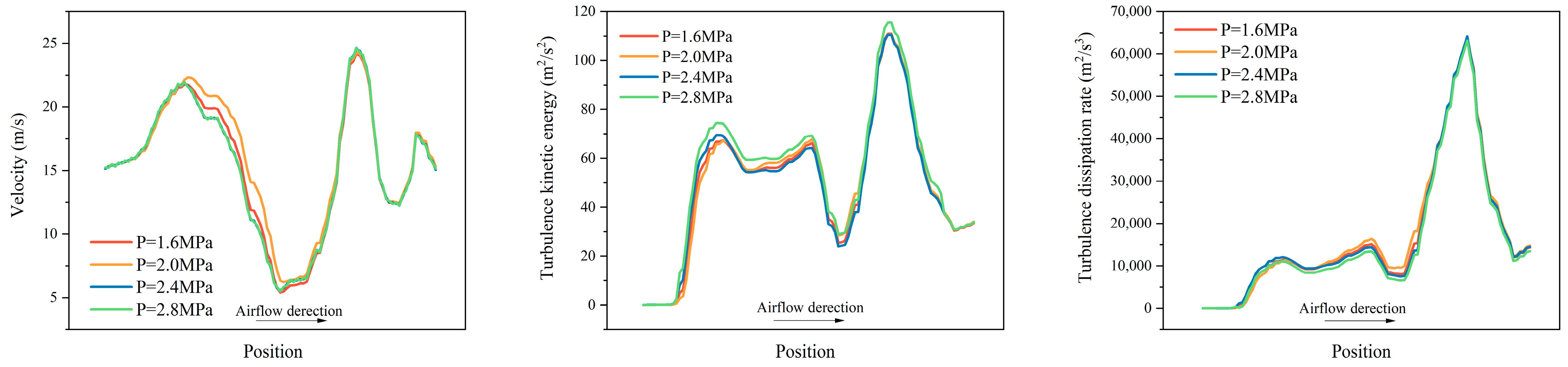
4.2. The Influencing Factors of Aerodynamic Noise Generation

Referring to the actual operating parameters of a natural gas transmission and distribution station in Southwest China, the impact of different operating conditions (gas flow velocity, outlet pressure, and valve opening) on aerodynamic noise was assessed by changing a single variable. When the valve opening and outlet pressure remained unchanged (100% and 2 MPa, respectively), and the inlet flow velocity increased from 6 m/s to 15 m/s at a rate gradient of 3 m/s, the maximum flow velocity inside the valve increased nonlinearly (as shown in Figure 8A). Simultaneously, with an increase in the inlet flow velocity, the fluid pressure undergoes significant changes. When the inlet flow velocity increased from 6 m/s to 12 m/s, the inlet static pressure increased by approximately 0.25 kPa for every 3 m/s increase, while from 12 m/s to 15 m/s, the inlet static pressure increased by 0.5 kPa. This is because the kinetic and potential energies of the fluid also increase as the flow velocity increases, and the increased potential energy is then converted into the pressure of the fluid. However, the distribution pattern of the pressure field inside the valve remains almost unchanged. The bottom of the valve chamber had more high-pressure areas than the top and was distributed in a circular pattern. Isobaric lines were dense at the throttle outlets and corners. Under different inlet flow velocities, many vortex rings with different structures were formed near the wall, and the vortex structures were mainly concentrated at the valve inlet, valve chamber, and throttle outlet (Figure 8B), with many vortex structures remaining at a certain distance after the outflow. This may be due to the fact that at lower flow velocity, although the fluid has less inertia, it is affected by wall obstruction and viscosity, resulting in unstable fluid flow and turbulence. At the same time, under high-speed flow conditions, the fluid has large inertia, resulting in uneven pressure and velocity, which also leads to turbulence. These results indicate that the inlet gas flow velocity significantly affects the internal flow field of the valve when the valve opening and outlet pressure remain unchanged.

Maintaining a constant inlet flow velocity (9 m/s) and valve opening (100%), the outlet pressure increased from 1.6 to 2.8 MPa at a rate gradient of 0.4 MPa to analyze the impact of changing the outlet pressure on the flow velocity. The results show that as the pipeline outlet pressure increases, both the magnitude and distribution of the flow velocity in the flow field and the internal vortex structure of the valve remain almost unchanged (Figure 9A,B). Figure 10 shows that the velocity, turbulent kinetic energy, and turbulent energy dissipation along the central streamline at different outlet pressures remained almost unchanged. These results indicate that, within the studied pressure range, the outlet pressure has a minimal impact on the internal flow field of the valve.

With a constant outlet pressure (2 MPa) and flow velocity (9 m/s), a valve opening change gradient of 20% was set to analyze its impact on the flow field velocity, as shown in Figure 11A. The results indicated that when the valve opening increased from 40% to 60%, the maximum fluid velocity rapidly decreased from 74 to 42 m/s. When the valve opening continued to increase to 80% and 100%, the maximum fluid velocity decreased to 37 m/s and 36 m/s, respectively, ultimately maintaining the stability. This may be because when the throttle window area is small at lower valve openings, the fluid requires higher flow velocities to meet the same flow rate demand. When the valve opening reaches a certain degree, no higher flow velocities are required to satisfy the flow rate demand. Moreover, the sizes of the vortex structures in region I (near the valve outlet) and region II (bottom of the valve chamber) underwent significant changes with increasing valve opening (Figure 11B). When the valve opening was 80%, the distribution of the vortex rings was the widest. These vortex structures influence fluid mixing and transport and can cause energy loss and noise generation [22,23]. These results indicate that the valve opening significantly impacts the internal flow field of the valve when the outlet pressure and flow velocity remain unchanged.

4.3. Acoustic Simulation

Figure 12 illustrates the distribution of aerodynamic noise sources on the symmetry plane of the flow channel when natural gas flows inside the valve under different operating conditions. In regions with higher sound power levels, the fluid velocity, turbulent kinetic energy, and turbulent dissipation rate inside the pipeline also increase accordingly. This indicates that a higher turbulence intensity and faster energy conversion in the flow channel increases the likelihood of aerodynamic noise generation. Compared with the distribution of vortex structures in the flow channel shown in Figure 7A, it can be observed that the area where vortex structures are formed has relatively high sound power levels in the flow channel, indicating that the formation and shedding of vortex structures also affect the generation of aerodynamic noise. Wei et al. [24] also compared the distribution of sound power levels with the distribution of fluid velocity and turbulence intensity, indicating that the alternating formation and shedding of vortices and shock waves in the pressure-reducing valve are the main causes of noise generation. Figure 13A illustrates the changes in the sound power levels along the flow direction of the natural gas inside the flow channel under different pipeline flow velocities. The results indicate that when the flow velocity increases from 6 m/s to 15 m/s in increments of 3 m/s, the maximum sound power level rises from 90.3 dB to 104.0 dB, 110.5 dB, and 116.2 dB, respectively. Although the sound power level inside the flow channel increases with increasing flow velocity, the rate of increase in the sound power level slows down. Increasing the flow velocity accelerates the irregular motion of fluid molecules and increases the frequency and energy transfer velocity of molecular collisions, resulting in larger pressure fluctuations and elevating sound energy and sound power levels inside the airflow. As the flow velocity continues to increase, the sound power released by the sound source gradually approaches saturation, and the rate of increase in the sound power level slows down or even stops increasing.

Figure 13B shows the changes in sound power levels along the central axis of the flow channel under different outlet pressures. The results indicate that when the outlet pressures are 1.6 MPa, 2.0 MPa, 2.4 MPa, and 2.7 MPa, the maximum sound power levels inside the flow channel are 103.4 dB, 104.1 dB, 103.8 dB, and 103.6 dB, respectively, showing less than 1% variation. This suggests that varying the outlet pressure did not significantly affect the maximum sound power level. Compared with Figure 10, it can be seen that under different outlet pressures, changes in velocity, turbulent kinetic energy, and turbulent dissipation rate inside the valve are not significant, indicating that outlet pressure variations have little effect on the flow field characteristics inside the valve and thus have almost no effect on the maximum sound power level.

Figure 13C illustrates the changes in the sound power levels along the central axis of the flow channel for different valve openings. The results show that at positions of 40%, 60%, 80%, and 100%, the maximum sound power levels inside the flow channel are 121.3 dB, 105.7 dB, 103.2 dB, and 104.0 dB, respectively. In the case of a smaller opening, the natural gas flow velocity at the throttle was higher, and the turbulent kinetic energy was greater, resulting in rapid energy conversion and an increase in the sound power level. As the opening gradually increased, the sound power level began to decrease, which may have been due to an increase in flow capacity at the throttle, a slowdown in natural gas flow velocity, and a weakening in turbulence intensity. When the valve opening exceeded 80%, the changes in the sound power level became insignificant. This may be attributed to the excessive flow area causing more oscillations and fluctuations in the fluid inside the flow channel, increasing the collision between fluid molecules, and thus raising the sound power level. However, Xu et al. [25] found in their study on the aerodynamic noise of control valves that with the increase in valve opening, the maximum sound pressure level of noise sources decreased nearly linearly to 121, 116, 89, and 81 dB, respectively. This is because the control valve in their study had a gate structure, and the valve control and fluid flow modes were different from the research object in this study. This indicates that the valve structure affected the aerodynamic acoustic characteristics.

4.4. The Characteristics of Propagation of Noise Outside the Valve

When the aerodynamic noise generated by the fluid inside the valve propagates outward, it can cause noise pollution outside of the valve. Sound pressure describes the properties of the sound field and typically varies with distance. Figure 14A illustrates the sound pressure fluctuations at monitoring points 1, 2, 8, and 12 m from the valve under different pipeline flow velocities. When v = 6 m/s, the sound pressure fluctuates periodically in a spindle shape between −28 and 28 Pa; when v = 9 m/s, it fluctuates periodically in a rectangular shape between −1 and 1 Pa; when v = 12 m/s and v = 15 m/s, it fluctuates in a sawtooth shape between −0.64 and 0.64 Pa. The results showed that as the flow velocity increased, the sound pressure peak decreased, and the fluctuation range narrowed. Drastic changes in flow velocity may cause refraction, reflection, and scattering of sound waves, thereby affecting the sound pressure distribution and propagation. Sound pressure may also be influenced by factors such as the Mach number and turbulence effects. Figure 14B illustrates the sound pressure fluctuations at monitoring points 1, 2, 8, and 12 m from the valve under different outlet pressures. When the outlet pressure is 1.6 MPa, the sound pressure fluctuates in a sawtooth shape between −0.48 and 0.48 Pa; at 2.0 MPa, it fluctuates in a rectangular shape between −1 and 1 Pa; at 2.4 MPa, it fluctuates in a spindle shape between −1.3 and 1.3 Pa; and at 2.7 MPa, it fluctuates in a sawtooth shape between −0.8 and 0.8 Pa. As the outlet pressure increases, the sound pressure peak first increases and then decreases, and the fluctuation range of the sound pressure first widens and then narrows. Figure 14C illustrates the sound pressure fluctuations at monitoring points 1, 2, 8, and 12 m from the valve under different valve openings. When the valve opening is 40%, the sound pressure fluctuates in a spindle shape between −0.8 and 0.8 Pa; at 60% and 80%, it fluctuates in a sawtooth shape between −0.6 and 0.6 Pa; and at 100%, it fluctuates in a rectangular shape between −1 and 1 Pa.

From Figure 14A–C, it can also be observed that when the sound pressure distribution is spindle-shaped, the sound pressure peak is relatively large; when it is rectangular, the sound pressure peak is moderate; and when it is sawtooth-shaped, the sound pressure peak is relatively small. Therefore, different pipeline flow velocities, outlet pressures, and valve openings can affect the shape of the sound pressure distribution and magnitude of the sound pressure peak, thus altering the propagation characteristics of the aerodynamic noise outside the valve. Moreover, under the same working conditions, the shape of the sound pressure fluctuation curve for different sound wave propagation distances was similar, and the sound pressure valve decreased almost linearly as the distance increased.

4.5. Directional Analysis of Aerodynamic Noise

Figure 15 illustrates the directional distribution of noise from the valve under various pipeline flow velocities. The results indicated that under different outlet pressures, flow velocities, and valve openings, the directional distribution of noise was symmetrical along the central axis of the flow channel, and the overall trend was similar. At a distance of 1 m from the valve, regions with high sound pressure levels were concentrated around 25°, 90°, 155°, 205°, 270°, and 335°; with a single-side radiation range of approximately 90°; and the directional distribution tended to be in the shape of a six-leaf flower shape. At a distance of 2 m from the valve, regions with high sound pressure levels were concentrated around 0°, 90°, 180°, and 270°; the radiation range was reduced to 50°; and the directional distribution tended to be in the shape of a four-leaf flower. This indicates that as the distance increased, the noise propagation became more focused and concentrated in the vertical and flow directions of the valve. Additionally, with constant outlet pressure and valve opening, when the fluid velocity increases from 6 m/s to 15 m/s in 3 m/s increments, the difference in sound pressure levels gradually decreases, indicating that the directional distribution of sound pressure levels gradually becomes uniform. With constant fluid flow velocity and valve opening, when the outlet pressure increases from 1.6 MPa to 2.8 MPa, the sound pressure level first increases and then decreases. With constant fluid flow velocity and outlet pressure, as the valve opening increased from 40% to 100%, the sound pressure level at the monitoring points first decreased and then increased, especially at 2 m. Notably, the sound pressure levels were very low at angles of 45°, 135°, 225°, and 315° relative to the valve–pipe connection. This may be due to obstacles encountered by sound waves when propagating in air, resulting in reflection, transmission, or diffraction. Owing to the inability of sound waves to reach behind obstacles, a sound-shadow area is formed, which is a typical interference effect in the sound field. The directional propagation of noise can spread further in specific directions and has a broader impact on the surrounding environment and humans. Therefore, in practical engineering applications, the directional noise of valves should be considered, and corresponding measures should be taken to reduce or control the propagation of noise in a specific direction.

5. Conclusions

In this study, the natural gas flow inside the (K)TS control valve was simulated under different operating conditions to analyze the characteristics of the gas flow field and sound field inside the valve. The mechanisms of aerodynamic noise generation inside the (K)TS control valve and its directional propagation characteristics are elucidated in detail. The main conclusions are as follows.

(1)

A grid cell size of 3.6 mm and boundary layer of 3 were used to ensure the accuracy of the 3D valve model calculations. The spectral curves of the measured aerodynamic noise data closely matched the simulation results, thus validating the effectiveness of the model.

(2)

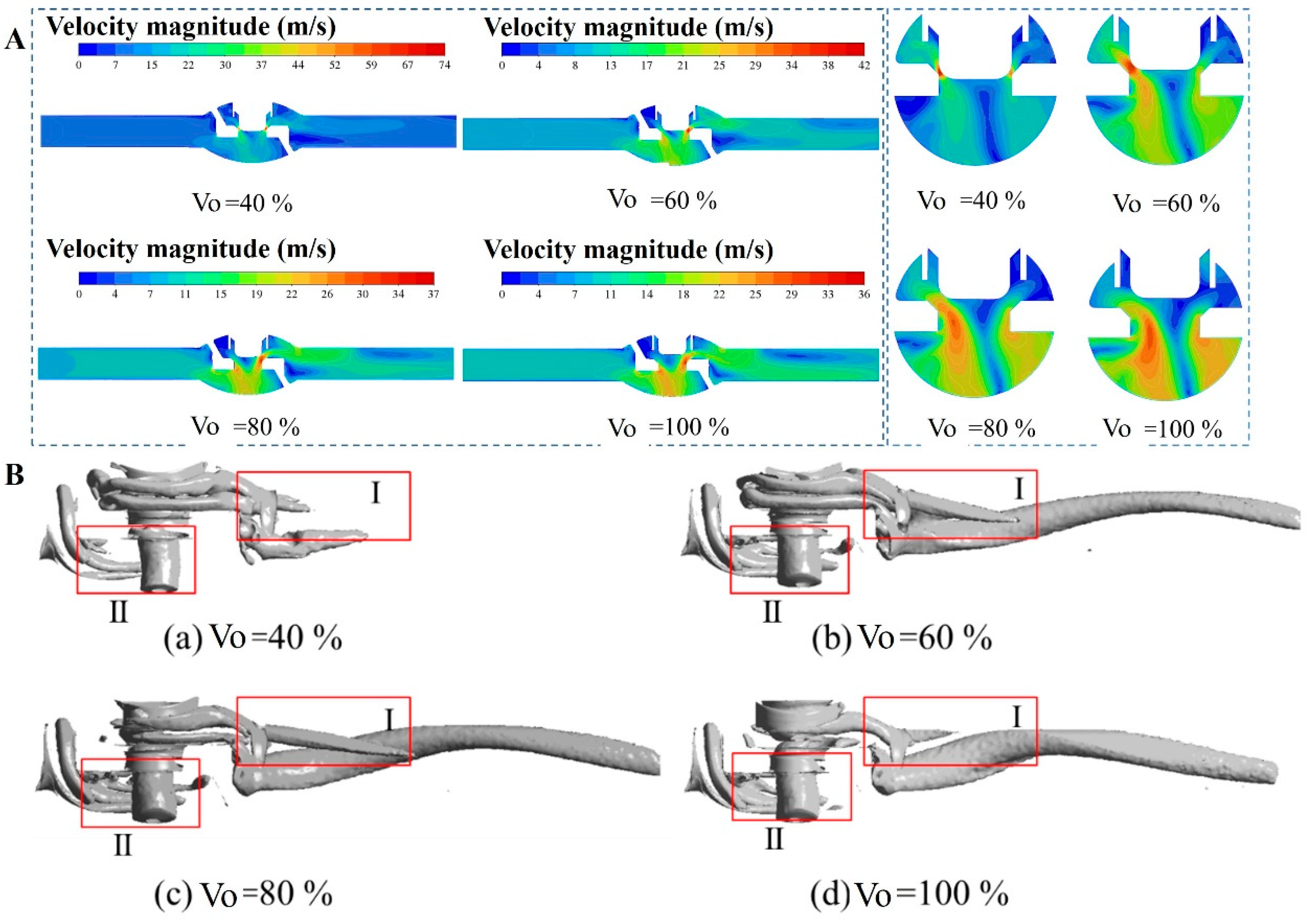
Increasing the pipeline inlet flow velocity leads to more intense turbulence and faster energy dissipation inside the valve, whereas the outlet pressure minimally affects the flow field characteristics. The valve opening primarily affected the size of the vortex rings at the valve chamber and throttle outlet.

(3)

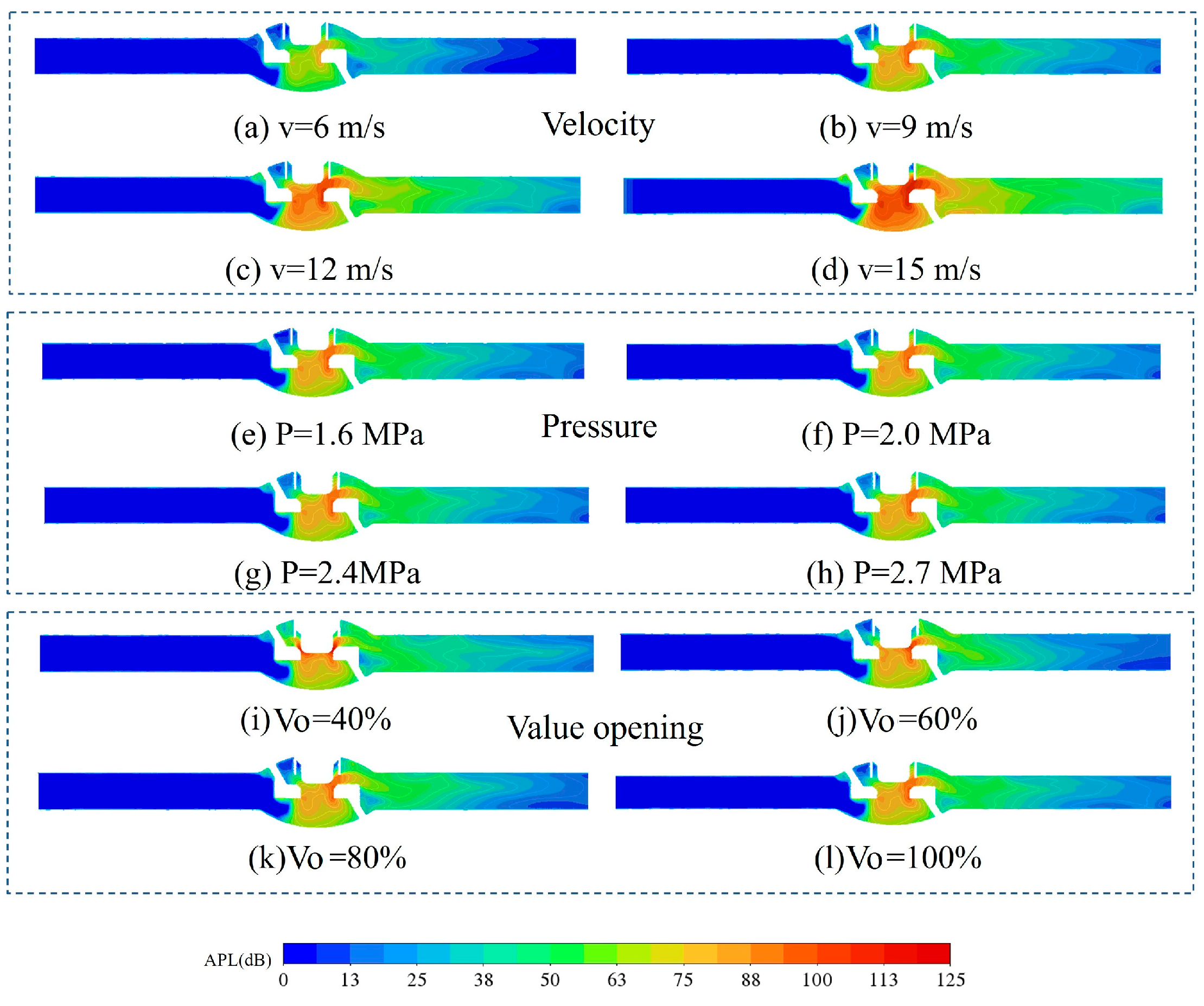
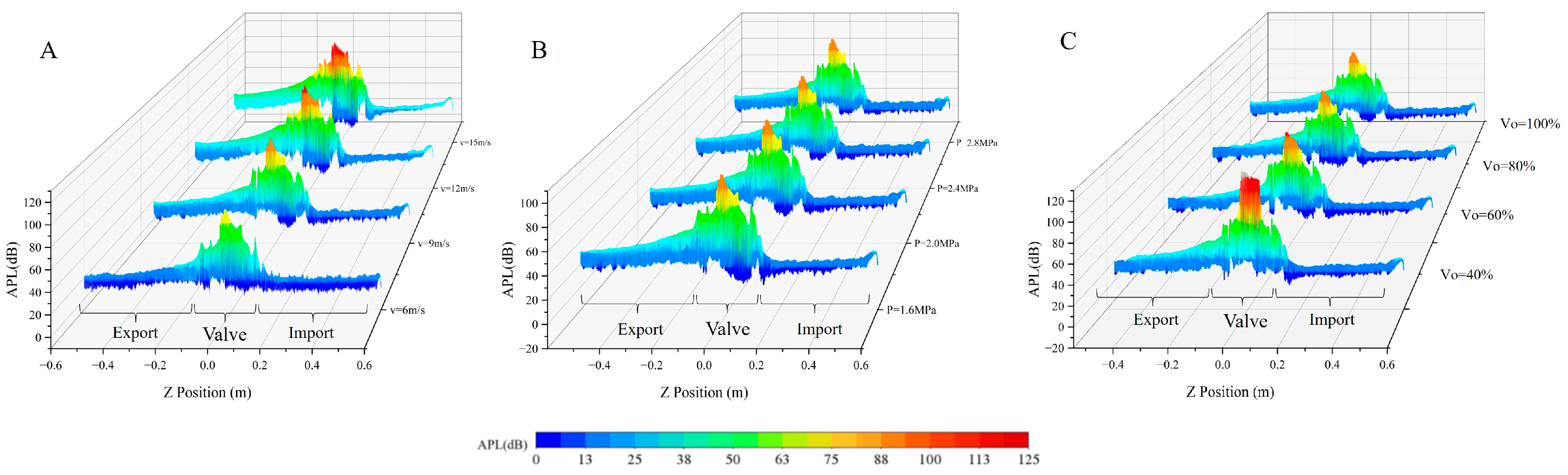
High flow velocity gradients, strong turbulence intensity, and rapid turbulent energy dissipation, along with vortex formation and shedding, were the primary causes of aerodynamic noise generated inside the valve. Noise-generating regions were primarily concentrated at the throttle port, valve chamber, and valve inlet.

(4)

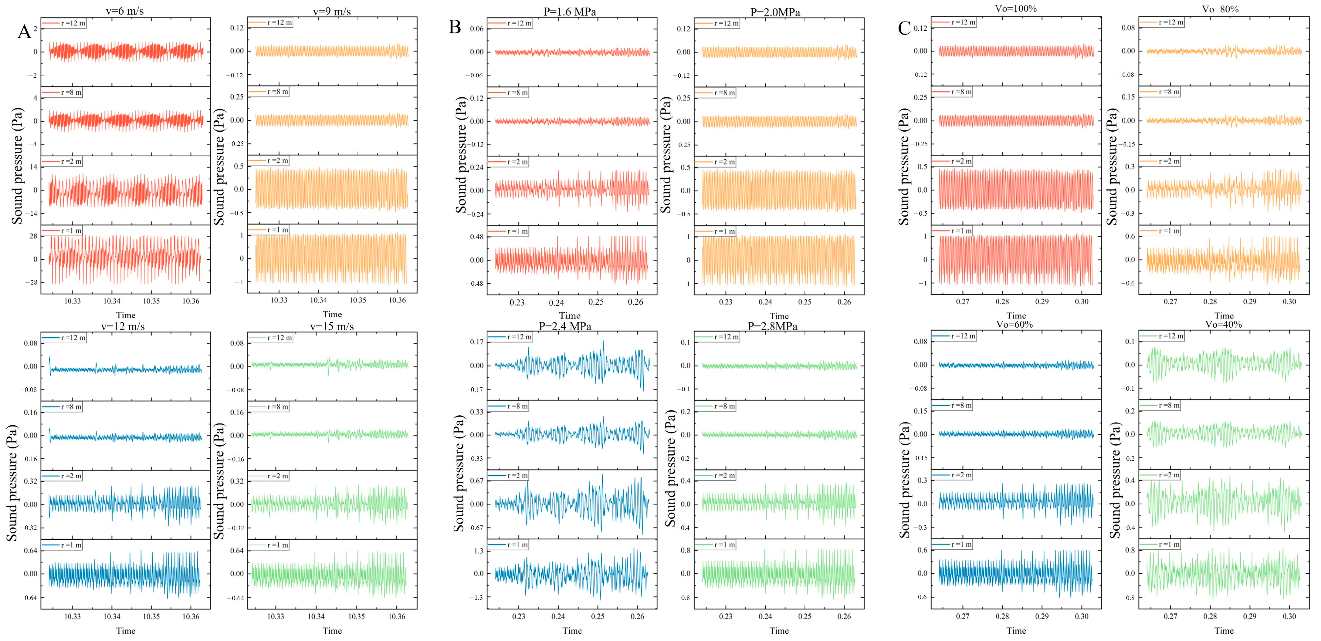
Under different operating conditions, the directional noise distribution was similar, exhibiting symmetry along the central axis of the flow channel, resembling six-leaf or four-leaf flower shapes. The aerodynamic noise of the valve propagated along the pipeline. However, with increasing distance, it became more concentrated in the vertical direction of the valve.

These results indicate that stabilizing the internal flow state of the valve and considering noise propagation in specific directions may be one of the key strategies to reduce the noise of (K)TS valves in natural gas transmission and distribution stations in Southwest China. These findings provide theoretical basis for understanding the mechanism of aerodynamic noise inside (K)TS control valves during the process of natural gas transmission and can guide the design of noise reduction products for (K)TS valve, which is useful for the prevention and control of noise pollution in natural gas transmission and distribution stations.

References

1. Thomson, H.; Corbett, J.J.; Winebrake, J.J. Natural gas as a marine fuel. Energy Policy 2015, 87, 153–167. [Google Scholar] [CrossRef]
2. Zhou, X.Y.; Wu, Y.S. A study of the similarity relationship in hydrodynamic noise. J. ACTA Acust. 2002, 27, 373–378. [Google Scholar]
3. Hays, J.; McCawley, M.; Shonkoff, S.B.C. Public Health Implications of Environmental Noise Associated with Unconventional Oil and Gas Development. Sci. Total Environ. 2017, 580, 448–456. [Google Scholar] [CrossRef] [PubMed]
4. Cinto, M.E.; McClure, C.J.W.; Barber, J.R. Large-scale Manipulation of the Acoustic Environment Can Alter the Abundance of Breeding Birds: Evidence from a Phantom Natural Gas Field. J. Appl. Ecol. 2019, 56, 2091–2101. [Google Scholar] [CrossRef]
5. Alzamzam, W.S.; Alfaghi, W.B. Noise Evaluation in Oil and Gas Fields and Associated Risk Assessment. Euro-Mediterr. J. Environ. Integrat. 2021, 6, 78. [Google Scholar] [CrossRef]
6. Liu, E.B.; Yan, S.K.; Peng, S.B.; Huang, L.Y.; Jiang, Y. Noise Silencing Technology for Manifold Fow Noise Based on ANSYS Fluent. J. Nat. Gas Sci. Eng. 2016, 29, 322–328. [Google Scholar] [CrossRef]
7. Su, Z.Y.; Liu, E.B.; Xu, Y.W.; Xie, P.; Shang, C.; Zhu, Q.Y. Flow Field and Noise Characteristics of Manifold in Natural Gas Station. Oil Gas Sci. Technol. 2019, 74, 70. [Google Scholar] [CrossRef]
8. Ma, D.Y.; Li, P.Z.; Dai, G.H.; Wang, H.Y. Pressure Dependence of Turbulent Jet Noise. Acta Phys. Sin. Ed. 1978, 2, 122–125. [Google Scholar]
9. Ma, D.; Li, P.; Dai, G.; Wang, H. Shock Associated Noise From Choked Jets. Acta Acust. 1980, 3, 172–182. [Google Scholar]
10. Zhao, M.; Liu, D.; Hou, J.; Zhang, X.; Li, S. Numerical Simulation of Inverted Bucket Steam Valve Noise Based on Multiband Analysis. J. Appl. Fluid Mech. 2024, 17, 1002–1014. [Google Scholar]
11. Shi, H.; Zhou, X.; Zhou, A.M.; Zhang, B.H.; Li, S.X. Numerical Simulation of Fluid-Solid Coupling Noise in Marine Three-Way Control Valve. J. Appl. Acoust. 2024, 43, 142–150. [Google Scholar]
12. Han, N.; Mak, C.M. Estimation of Breakout Sound Power Level due to Turbulence Caused by an In-Duct Element. Tech. Acoust. 2007, 5, 653–657. [Google Scholar]
13. Williams, J.E.F.; Hawkings, D.L. Sound Generation by Turbulence and Surfaces in Arbitrary Motion. Philos. Trans. R. Soc. A 1969, 264, 321–342. [Google Scholar]
14. Li, Y.A.; Cui, W.Z.; Jiang, X.F.; Li, L.J.; Liu, J.F. Numerical Study of Thermal and Resistance Characteristics in the Vortex-Enhanced Tube. Energies 2025, 18, 13. [Google Scholar] [CrossRef]
15. Yan, S.K.; Li, C.J.; Xia, Y.F.; Li, G.L. Analysis and Prediction of Natural Gas Noise in a Metering Station Based on CFD. Eng. Fail Anal. 2020, 108, 104296. [Google Scholar] [CrossRef]
16. Zhang, N.; Xie, H.; Wang, X.; Wu, B.S. Computation of Vortical Flow and Flow Induced Noise by Large Eddy Simulation with FW-H Acoustic Analogy and Powell Vortex Sound Theory. J. Hydrodyn. 2016, 28, 255–266. [Google Scholar] [CrossRef]
17. Tan, J.; Dong, P.; Gao, J.; Wang, C.; Zhang, L. Coupling Bionic Design and Numerical Simulation of the Wavy Leading-Edge and Seagull Airfoil of Axial Flow Blade for Air-Conditioner. J. Appl. Fluid Mech. 2023, 16, 1316–1330. [Google Scholar]
18. Hou, J.J.; Li, S.X.; Yang, L.X.; Liu, D.; Zhao, Q. Numerical Simulation and Reduction of Balance Valve Noise Based on Considering Quadrupole and Dipole in Different Frequency Bands. Appl. Acoust. 2023, 211, 109504. [Google Scholar] [CrossRef]
19. Li, S.X.; Hou, J.J.; Pan, W.L.; Wang, Z.H.; Kang, Y.X. Study on Aerodynamic Noise Numerical Simulation and Characteristics of Safety Valve Based on Dipole and Quadrupole. Acoust. Aust. 2020, 48, 441–454. [Google Scholar] [CrossRef]
20. Huang, J.Y.; Zhang, K.; Li, H.Y.; Wang, A.R.; Yang, M.Y. Numerical Simulation of Aerodynamic Noise and Noise Reduction of Range Hood. Appl. Acoust. 2021, 175, 107806. [Google Scholar] [CrossRef]
21. Sun, L.H.; Zhe, C.T.; Guo, C.; Cheng, S.; He, S.Y.; Gao, M. Numerical Simulation Regarding Flow-Induced Noise in Variable Cross-Section Pipelines Based on Large Eddy Simulations and Ffowcs Williams—Hawkings Methods. AIP Adv. 2021, 11, 065118. [Google Scholar] [CrossRef]
22. Jia, J.B.; Shi, Y.; Meng, X.Y.; Zhang, B.; Li, D.M. Pneumatic Noise Study of Multi-Stage Sleeve Control Valve. Processes 2023, 11, 2544. [Google Scholar] [CrossRef]
23. Guo, G.; Zhu, L.; Xing, B.Y. Density Distribution Characteristics of Fluid Inside Vortex in Supersonic Mixing Layer. Acta Phys. Sin. 2020, 69, 144701–144715. [Google Scholar] [CrossRef]
24. Wei, L.; Zhang, M.; Jin, Z.J.; Chen, L.L. Numerical Analysis of Aerodynamic Noise in a High Parameter Pressure Reducing Valve. Appl. Mech. Mater. 2013, 397–400, 274–277. [Google Scholar] [CrossRef]
25. Xu, W.W.; Wang, Q.G.; Wu, D.Z.; Li, Q. Simulation and Design Improvement of a Low Noise Control Valve in Autonomous Underwater Vehicles. Appl. Acoust. 2019, 146, 23–30. [Google Scholar] [CrossRef]
Figure 1. Valve structure (A) and the positive profile of valve pipeline and flow channel extraction (B).
Energies 18 00968 g001
Figure 2. Schematic diagram of simulation calculation process.
Energies 18 00968 g002
Figure 3. The polyhedral grids of flow channel (a, b, c, d, e, f, and g represent grids 1, 2, 3, 4, 5, 6, and 7, respectively).
Energies 18 00968 g003
Figure 4. The variation of flow rate and the calculated deviation with the number of grids.
Energies 18 00968 g004
Figure 5. Comparison of the SPL between simulation and actual measurement at a distance of 1 m from the valve.
Energies 18 00968 g005
Figure 6. (A) Velocity profile of different sections in the flow channel. (B) Static pressure distribution diagram of different sections. (C) Dynamic pressure distribution diagram of different sections.
Energies 18 00968 g006
Figure 7. (A) The vortex structure in flow channel. (B) The distribution of turbulent kinetic energy and turbulent dissipation rate at section.
Energies 18 00968 g007
Figure 8. (A) Velocity profile of different sections in the flow channel. (B) Vortex structure under different inlet flow velocities.
Energies 18 00968 g008
Figure 9. (A) Velocity distribution at section X = 0 under different outlet pressures. (B) Vortex structure under different outlet pressures.
Energies 18 00968 g009
Figure 10. Changes in velocity (A), turbulence kinetic energy (B), and turbulence dissipation rate (C) on streamlines under different outlet pressure.
Energies 18 00968 g010
Figure 11. (A) Velocity distribution of different valve positions at section X = 0 and Z = 0. (B) Vortex structure with different valve openings.
Energies 18 00968 g011
Figure 12. Sound power level distribution at section X = 0 under different operating conditions.
Energies 18 00968 g012
Figure 13. Sound power levels varying with Z-coordinates under different operating conditions: (A) sound power levels at different pipe flow velocities; (B) sound power levels at different outlet pressures; (C) sound power levels with different valve openings.
Energies 18 00968 g013
Figure 14. (A) Time-domain fluctuation distribution of sound pressure under different flow velocities. (B) Time-domain fluctuation distribution of sound pressure under different outlet pressures. (C) Time-domain fluctuation distribution of sound pressure with different valve openings.
Energies 18 00968 g014
Figure 15. Directional analysis of noise under different flow velocities, outlet pressures, and valve openings.
Energies 18 00968 g015