Abstract
The performance of a conventional Ground-Source Refrigeration and Air Conditioning (GSRAC) system with a borehole heat exchanger (BHE) can be enhanced by addressing the soil thermal imbalance issue that affects these systems. This study proposes a novel concept for seasonal cold energy storage using a Thermal Diode Tank (TDT). The TDT consists of an insulated water tank fitted with an array of heat pipes. By integrating the TDT into a conventional GSRAC system, “cold” energy can be passively collected from ambient air during winter, injected into the BHE, and stored in the soil. The stored “cold” energy can then be retrieved in the summer, facilitating cross-seasonal cold energy storage (CS). Thus, a conventional GSRAC system can be transformed into a GSRAC system with cross-seasonal cold energy storage capability, i.e., GSRAC + CS system. The validated BHE model previously developed by the authors is used to predict the performance improvements achieved using the GSRAC + CS system. The results indicate that the Annual Net Cold Energy Storage Efficiency (ANESE) increased from 5.7% to 10.7% over a ten year period. The average Borehole Performance Improvement (BPI) due to the addition of cold storage capability is 11% over the same timeframe. This study also discusses the impacts of varying design and operational parameters on ANESE and BPI. The results demonstrate that GSRAC + CS systems not only mitigate the soil thermal imbalance issue faced by conventional GSRAC systems, but also require less BHE depth to achieve equivalent performance.
1. Introduction
Over the past century, there has been a dramatic increase in demand for space cooling [1]. This demand has been even more rapidly grown over the past decade because of new, emerging, largely cooling-dominant applications, namely cold facilities for vaccine and food storage [2]. One promising approach to address this growing demand is to make use of seasonal temperature changes; therefore, several studies have been conducted to investigate this approach to cooling buildings [3,4,5].
The sources of seasonal cold storage can be in the form of snow, cold air, or low-temperature water, which are widely available in relatively cold regions [6]. However, one of the primary challenges is the possibility of storing this energy for extended periods of time [7]. More recent attention has focused on enabling the storage of these sources for space cooling [8]. Borehole Thermal Energy Storage (BTES) systems have the potential to store thermal energy during offseason periods [9].
Utilising BTES systems can help reduce the energy consumption of cooling-dominant applications by making use of underground thermal reservoirs as heat sinks for refrigeration and air conditioning (RAC) systems [10]. An underground thermal reservoir has a relatively stable temperature, unlike ambient air temperature [11]. Therefore, BTES system can be used to enhance the efficiency of cooling facilities by exchanging heat with underground thermal reservoirs. However, where cooling alone is required, the continuous use of underground thermal reservoirs as heat sinks in cooling applications may potentially cause soil thermal imbalance issues [12]. The soil temperature near the borehole heat exchanger (BHE) may increase over the lifetime of the system, thereby reducing the efficiency of the air conditioning system [13]. Several research studies have addressed the issues associated with unbalanced thermal loading and performance degradation in BHEs [14].
One widely used approach to reduce the soil thermal imbalance problem is certain design solutions, which, for example, may include increasing the spacing between BHEs and BHE depth. However, these measures may lead to a significant increase in the system installation cost and the size of the system, which would require a larger area. The latter may not be readily available in urban environments [15].
Another approach is to utilise the supplementary heat rejection equipment to reject the accumulated underground heat to maintain the ground in thermal equilibrium. Rejection of the accumulated heat of the ground leads to a higher temperature difference between the BHE wall and the ground, thereby increasing the efficiency of BHEs [16]. Although several technologies have been proposed for BHEs in heating-dominated applications, such as waste-heat utilisations [17], supplementary boilers [18], solar collectors [19], and air sources [20], only cooling towers and dry-air coolers [21] have been proposed for BHEs in cooling-dominated applications. Cooling towers dissipate the accumulated heat via the evaporation of water, which is sprayed on the outer surface of the pipe, whereas dry-air coolers rejects heat by causing air to move across the carrier fluid [22]. The efficacy advantages associated with using cooling towers and dry-air coolers in BTES systems can be limited once their energy and water consumptions exceed their potential energy savings [23]. The literature offers no guidance on passive solutions (like solar collectors in heating-dominated applications) for the problem of soil thermal imbalance in cooling-dominated applications. In addition, there is a gap in the literature regarding the coupled system for seasonal and diurnal cooling, as revealed in [24]. Consequently, this paper aims to fill this gap by proposing a new passive seasonal cold storage concept to address the problems faced by conventional GSRAC systems, i.e., soil thermal imbalance and performance deterioration. The new concept is expected to further improve the efficiency of GSRAC systems operating in cooling-dominated applications.
The basic concept suggested in this work is to utilise a passive supplementary heat rejection module, a Thermal Diode Tank (TDT), to collect the seasonal cold energy from the cold ambient air and use it to extract the accumulated heat from the soil. The TDT is made from an array of thermosyphon heat pipes and a water tank. It serves as a Cold Storage (CS) unit. By integration of the GSRAC system into the CS unit, the seasonal cold energy can be harvested and stored in the soil in winter and recovered in summer to achieve utilisation of cross-seasonal energy. The proposed CS facility, the TDT, can potentially be a more efficient alternative to cooling towers and dry-air coolers. The advantages of the proposed system mainly rely on the fact that it does not require any external energy or water supply [4,25]. Ultimately, this paper aims to theoretically demonstrate the advantages of an integrated GSRAC system with CS unit (GSRAC + CS) in terms of the improvement of the overall system performance.
The structure of this paper is as follows: In Section 2, the description of the proposed system is presented. In Section 3, the simulation method and the main input parameters are provided. In Section 4, a comparison between the GSRAC system with CS facility (GSRAC + CS) and the conventional GSRAC system in terms of their soil temperature profiles, ANESE, and BPI is performed. In Section 5, the impacts of changing the parameters affecting the GSRAC + CS performance are analysed. The main findings and conclusions are outlined in Section 6.
2. GSRAC + CS System
2.1. The Conventional GSRAC System
A conventional GSRAC incorporates a refrigeration and air conditioning (RAC) system with a single BHE. The BHE harvests the (cold) energy from the relatively low subsurface ground temperature in summer to enhance system performance. A conventional GSRAC system typically includes a BHE that is connected to the RAC unit. This system consists of two flow loops, namely the RAC and BHE loops, which are dedicated to the space cooling system during warm seasons, as shown in Figure 1.
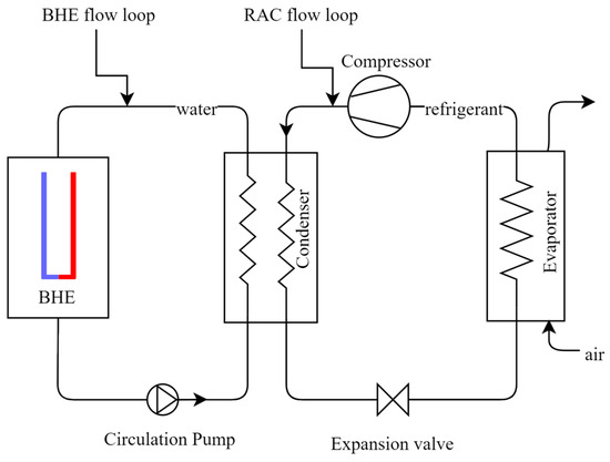
Figure 1.
The Ground Source Refrigeration and Air Conditioning system (GSRAC).
2.2. Thermal Diode Tank (TDT)
A TDT consists of an insulated water tank beneath or above ground and heat pipes, as shown in Figure 2. It is built as a thermal diode, so it allows heat transfer in only one direction, i.e., it can only release heat to the environment when the water temperature is higher than the ambient temperature, but it does not absorb heat from the environment, even when the ambient temperature is higher than that of the water inside the tank. Being an insulated passive system, the TDT consumes no water and operates at no cost. Another important advantage is that it does not need maintenance after installation.
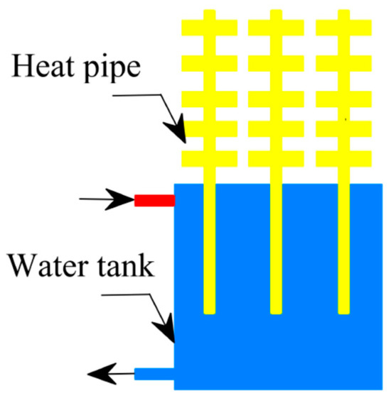
Figure 2.
Schematic of a Thermal Diode Tank (TDT).
2.3. The Proposed GSRAC + CS System
To reduce the thermal imbalance of conventional GSRAC systems used in warm regions, a cold energy storage (CS) unit based on heat pipes is proposed. The GSRAC + CS technology is a hybrid of the TDT and GSRAC, as illustrated in Figure 3. The proposed system consists of three flow loops, namely the RAC, BHE, and TDT flow loops. The RAC-BHE flow loops are dedicated to the space cooling system during warm seasons, while the BHE-TDT flow loop is used for “cold” energy charging during cold seasons.
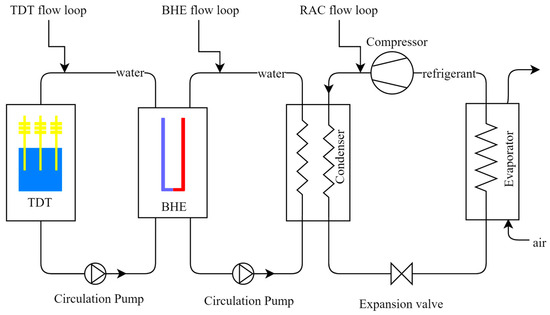
Figure 3.
The proposed Ground Source Refrigeration and Air Conditioning system with cross-seasonal Cold energy Storage capability (GSRAC + CS).
In winter, water circulates between the TDT and BHE, while the RAC system is not functioning (refer to Figure 4a). The TDT passively reduces the water temperature inside the tank to the same level as the minimum ambient temperature. This process, as mentioned above, does not need any additional energy supply. The low-temperature water is then injected into the soil through the existing BHE of the GSRAC system, thereby storing chilled energy in the soil. The stored energy then can be recovered and used in warm seasons by circulating water between the BHE and the RAC system (refer to Figure 4b). The GSRAC + CS system, therefore, has a cross-seasonal “cold” energy storage (CS) capability. The TDT can also harvest day/night ambient temperature fluctuations during summer to enhance the performance of the RAC system; however, the diurnal energy storage of TDT is beyond the scope of this paper.
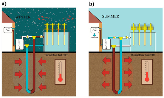
Figure 4.
A schematic diagram of the GSRAC + CS’s working principle during (a) charging operation; (b) discharging operation.
3. Calculation Method and Input Parameters
3.1. Calculation Method
The outlet water temperature from the BHE and the soil temperature are simulated using the Borehole Field-MATLAB based Programme (BMP), which was developed and validated previously by the current authors [26]. The model, which is based on the BMP, considers seasonal soil temperature fluctuations by integrating an internal heat source term concept [27] to the governing equations. In this model, the soil domain is modelled using a three-dimensional finite-difference approach, whilst a quasi-steady-state model is employed to model the heat transfer inside the BHE. The model output includes the temperature profiles of the soil, working fluid, and BHE wall. These outputs were validated against several published experimental studies in [26].
The water temperature on entry to the BHE during the discharging period (), i.e., summer seasons, depends on the refrigeration and air conditioning system’s performance. Therefore, this variable is set as the input parameter for the simulations.
The entering water temperature to the BHE during the “cold” energy charging period (), i.e., winter seasons, is assumed to be the average water temperature inside the water tank. This parameter depends on the ambient air temperature () and the thermal capacity of the TDT. The thermal capacity of a TDT is its ability to achieve a certain temperature difference () between the water inside the TDT and the ambient air. To simplify the problem, the variable is set as the input parameter in the simulations, and then the number of heat pipes required to achieve this temperature difference is calculated. Thus, the inlet water temperature to the BHE during the charging period can be written as follows:
To determine the required number of thermosyphon heat pipes to achieve the temperature difference of , a simple model based on energy balance is developed. The description of this model is provided in Appendix A.
3.2. Case Study
3.2.1. Borehole Heat Exchanger (BHE)
In this study, a single BHE with an effective depth of 80 m, which is typically used in Australia [28], is considered. A single U-tube pipe with an inner and outer radius of 0.013 m and 0.017 m and a half shank spacing of 0.025 m is inserted into the BHE with a radius of 0.055 m. Then, the BHE is filled with grouting material with a thermal conductivity of 1.4 W/(m K). The soil thermal conductivity and its volumetric heat capacity are assumed to be 1.5 W/(m K) and 3.2 MJ/(m3 K), respectively. The average undisturbed soil temperature along the BHE depth is set at 20.5 °C.
3.2.2. Thermal Diode Tank (TDT) Used in the Study
The TDT, as explained previously, is used to accumulate “cold” energy in the form of low-temperature water. The heat extraction inside the TDT is realised using heat pipe modules. Heat pipes are reorganised as passive heat transfer devices that efficiently move heat in only one direction [29]. The extracted heat in the TDT depends on the number of heat pipes and ambient weather conditions (temperature and wind). To reduce energy losses from the TDT, the tank is insulated using materials with low thermal conductivity. The heat pipe considered in this study is made from stainless steel with thermal conductivity of 15 W/(m K) and partially filled with the refrigerant R134a. The condenser and evaporator lengths of the heat pipe module are assumed to be 1 m and 2 m, respectively. The condenser section consists of 30 Aluminium fins with 200 mm diameter and 1 mm outer diameter. The inner and outer radii of the heat pipe are 8.5 mm and 9.1 mm, respectively. The heat transfer coefficient of the heat pipe between the inner wall and refrigerant is 900 W/(m2 K), and the heat transfer coefficient between the outer wall of the evaporator and water inside the tank is 200 W/(m2 K). The ambient temperature and wind speed in the charging seasons are assumed to be 8 °C and 5.5 m/s, respectively. Using Equations (A3)–(A8) in Appendix A, the values of thermal resistances are calculated and listed in Table 1.

Table 1.
The calculated thermal resistances of the heat pipe module.
Using Equation (A13), the required number of heat pipe modules to reject the accumulated underground heat with various values of is calculated and presented in Figure 5.
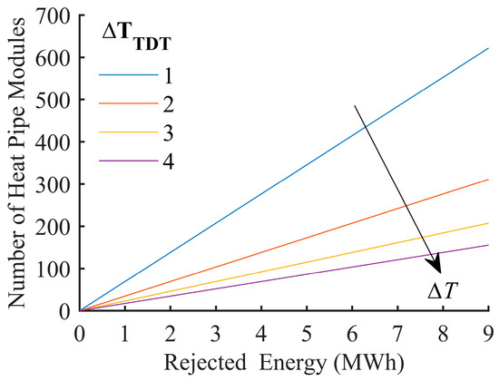
Figure 5.
Heat pipe module requirements for TDT with respect to the rejected accumulated energy. The arrow indicates the ascending order of .
3.2.3. Operation Schemes
Two different thermal load scenarios are examined: the scenarios with and without the “cold” energy storage. It is assumed that in the system with the CS, there is a sufficient heat transfer capacity for the TDT, so the water temperature inside TDT can be maintained (in winter) at 3 °C above the ambient temperature all the time. In other words, the number of heat pipes inside the TDT is selected so that a temperature difference of 3 °C between the water inside the tank and the ambient air can be achieved. The average minimum ambient temperature in winter (June–August in Adelaide, Australia), i.e., the cold energy charging (into soil) period, is assumed to be 8 °C [30]. In summer (December–February), the GSRAC and the GSRAC + CS systems are operated.
The baseline scenario with heat rejection is for the GSRAC system equipped with TDT. In summer, the condensing heat is injected through the BHE into the soil. In winter, the heat is extracted/discharged from the soil by circulating the low-temperature water provided by the TDT through the BHE. In summary, the operational scheme for the GSRAC + CS system is the following:
- In winter (June–August), from days 1 to 92, water circulates between the TDT and BHE. The inlet water temperature to the BHE is assumed to be 3 °C more than the average ambient temperature in winter.
- In spring (September–November), from days 93 to 183, the BHE is out of operation.
- In summer (December–February), from days 184 to 273, water circulates between the RAC and BHE. The inlet water temperature to the BHE is assumed to be 40 °C.
- Afterwards (March–May), from days 274 to 365, the BHE is out of operation.
Meanwhile, the operational scheme for the conventional GSRAC system, i.e., the baseline scenario without heat rejection, is the following:
- In summer (December–February), from days 184 to 273, water circulates between the RAC and BHE. The inlet water temperature to the BHE is assumed to be 40 °C, the same as that in the GSRAC + CS case.
- At other times, the BHE is out of operation.
Table 2 summarises the main parameters used for the case study and simulations.
Table 2.
The main simulation parameters.
3.3. Energy Storage Performance Evaluation Criteria
To evaluate the energy storage and performance of the BHE, three criteria of volumetric average soil temperature, annual net energy storage efficiency, and borehole performance improvement are defined and utilised in the current study. The volumetric average soil temperature determines the ability of a storage media to keep the “cold” energy within the storage region. The annual net energy storage efficiency determines the efficiency of the system to inject the extracted energy from the BHE during winter and summer. The borehole performance improvement determines the enhancement in thermal performance of the BHE due to the “cold” energy charging.
3.3.1. Volumetric Average Temperature (VAT)
The Volumetric Average Temperature (VAT) of the soil storage region is used as the “cold” energy charging performance indicator. This parameter is used to indicate the average soil temperature around the BHE at a particular time. The Volumetric Average (soil) Temperature (VAT) can be evaluated as follows:
where is the volume of the storage region, is the temperature of this control volume, and is the infinitesimal volume. A lower VAT at the beginning of summer is preferable because it implies a higher heat transfer rate between the BHE and the soil, thus improving the performance of the RAC unit during the cooling seasons.
To calculate the VAT, the volume of the storage region needs to be identified. The extent of the simulation domain in the BMP is evaluated, based on the Eskilson [31] approach, as follows:
where is the maximum distance to which the heat released by a line source (m) can be transmitted, is the thermal diffusivity of the soil (m2/s), and is the simulation time (s). For the reference case, the radius of the simulation domain is calculated based on 10 years of simulation time to eliminate the boundary effect after 10 years, i.e., substituting = 315,360,000 (s) in Equation (3). However, the radius of the storage region is taken as half of the maximum radius () for 3 months of simulation time, which is equal to the duration of the heat injection period at each year cycle. The reason is that the maximum temperature gradient occurs within the inner half of . The thermal diffusivity of soil is taken as 4.6 × 10⁻⁷ m2/s in this study. As a result, the radius of the simulation domain and storage region are 41.70 m and 2.85 m from the surface of the BHE, respectively, as shown in Figure 6.
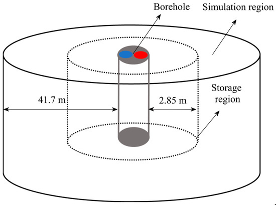
Figure 6.
Schematic of the simulation and “cold” storage regions.
3.3.2. Annual Net Energy Storage Efficiency (ANESE)
The Annual Net Energy Storage Efficiency (ANESE) is accepted in this work as the basic performance improvement indicator. This parameter is used to estimate the useful stored energy that can be extracted from the system. As given in Equation (4), the ANESE due to the hybrid effect was defined as the ratio of the increase in the injected heat during discharging period to the extracted heat during the charging period. The higher the ANESE is, the more extracted heat can be injected. Namely, the ANESE in year i is the following:
The “cold” energy charged in (heat extraction) in winter and the discharged out (heat injection) in summer are calculated by considering the temperature differences between the inlet and the outlet of the BHE and the mass flow rates through the BHE, as follows:
and
In the above equations, denotes the heat extracted from or the “cold” energy charged into the soil during the charging period, and and denote the heat injected into or the “cold” energy discharged from the soil during the discharging period of the GSRAC + CS and GSRAC systems, respectively. The variables and are the start time of charging and discharging periods, respectively. The variables and are the end time of the charging and discharging periods, respectively.
It should be noted that the current definition of the ANESE parameter in this paper is different from the energy storage efficiency used in [32,33]. Here, the ANESE represents the enhancement in the energy storage efficiency due to the hybridisation only, while in the mentioned references, the energy storage efficiency includes the enhancement achieved from both the hybridisation and natural recovery of soil temperature.
3.3.3. Borehole Performance Improvement (BPI)
The Borehole (thermal) Performance Improvement (BPI) is utilised to indicate the improvement of borehole performance. The BPI can be calculated as the ratio of the fluid temperature difference at the BHE outlet of the GSRAC and GSRAC + CS systems to that of between the BHE inlet and outlet of the GSRAC system. It is used to evaluate the effect of cold energy charging on the overall performance of the BHE. The Borehole Performance Improvement (BPI) in year can be evaluated as follows:
where and are the average outlet temperatures from the BHE of the GSRAC and GSRAC + CS systems during the “cold” energy discharging of year , respectively. The parameter is the inlet temperature to the BHE of GSRAC during the “cold” energy discharging of year , which was assumed to be 40 °C in this study.
4. Performance of the GSRAC + CS System
In this section, the performance of GSRAC and GSRAC + CS systems are compared, based on the developed simulation approach in terms of their soil temperature profiles (VAT), ANESE, and BPI for ten years.
4.1. Soil Temperature Profile
To understand the natural and forced recovery of the storage region, the soil temperature profiles of the baseline scenario without and with heat rejection (the GSRAC and GSRAC + S systems) at the beginning of the discharging phase (day 184) are simulated. The outcomes are illustrated in Figure 7. In the cold storage field, the VAT of the GSRAC system continuously increased from 20.92 °C to 22.14 °C over ten years, while for the GSRAC + CS system, the increase in VAT was much less (20.97 °C) after ten years, indicating that there would be a less severe thermal imbalance issue with GSRAC + CS system. In particular, the lower VAT would be better for the RAC system, since the rate of heat transfer between the soil and the BHE increases; therefore, a higher amount of heat can be injected into the ground. Therefore, in the GSRAC + CS system, the BHE can be operated sustainably for extended periods, while, for the GSRAC system, the performance of the BHE and RAC unit deteriorated over time.
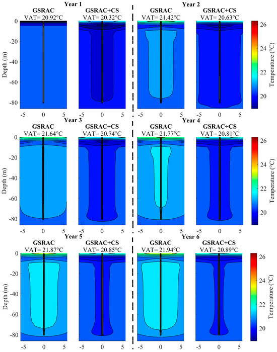
Figure 7.
The soil temperature profiles for a system with and without CS capability at the beginning of summer (after the first hour of pump operation) over a 10-year simulation. VAT indicates the average soil temperature over the storage region.
Figure 8a presents the outcomes of the simulation for the soil temperature difference between the GSRAC and GSRAC + CS systems at different distances from the BHE wall in the transverse direction at the end of the summer seasons. As can be seen, the maximum temperature difference occurred at around 3 m to the BHE wall, and it progressively increased from year to year. The results suggest that the bulk of thermal energy is stored in the 2–3 m zone around the BHE, implying that the radius of 2.85 m for the storage volume, which is considered in the simulations, is appropriate. A temperature comparison of the soil between GSRAC and GSRAC + CS systems indicates that the difference in temperature distribution between two systems increased gradually over the time from <0.3 °C in first 2 years to >0.9 °C in year 10. Figure 8b presents the soil temperature difference between GSRAC and GSRAC + CS systems at different distances from the bottom end of the BHE in the vertical direction at the end of the summer seasons. As opposed to the temperature difference in the transverse direction, the maximum temperature difference in the vertical direction occurs at around 0.3 m from the bottom end of the BHE, implying that the cold losses from the storage region in the vertical direction are much slower than those in the transverse direction. The temperature increase in the storage region would become even more significant when a high amount of heat would be injected into the soil. After being integrated with the TDT, the GSRAC system can maintain a good thermal balance and a stable soil temperature. Thus, the main result of these simulations is that the problem of soil thermal imbalance in cooling-dominated applications can be mitigated by integrating GSRAC systems with TDT units.
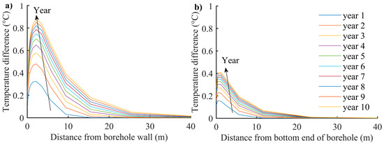
Figure 8.
The soil temperature difference between GSRAC and GSRAC + CS system at the end of summer over a simulation time, (a) at different distances from the BHE wall in the transverse direction, and (b) at different distances from the bottom end of the BHE in the vertical direction. The arrows indicate the ascending order of the year.
4.2. Annual NET Energy Storage Efficiency (ANESE)
Figure 9 shows the ANESE during each year of the ten-year simulation period. The results indicate that the proposed GSRAC + CS system can achieve a performance improvement of about 6% in the first year; moreover, it increases to more than 10% after ten years. This performance improvement is attributed to the difference of 0.07 to 0.92 °C in the outlet fluid temperatures between the GSRAC and GSRAC + CS systems during discharging seasons. Although this performance improvement may not be considered to be very significant, it may indeed be very essential if the rejected heat is achieved from a passive strategy, i.e., using the TDT.
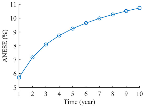
Figure 9.
Variations in the annual net energy storage efficiency (ANESE).
4.3. Results of Borehole Performance Improvement (BPI)
Figure 10 presents the fluid temperature difference between the BHE inlet and outlet for the GSRAC and GSRAC + CS systems in black (left axis) and BPI in blue (right axis) during each year of a simulation. What can be clearly seen in this figure is the rapid decrease in the fluid temperature difference between the BHE inlet and outlet of the GSRAC system from approximately 3.70 °C to 3.46 °C during the system operation. By contrast, in the GSRAC + CS system, the fluid temperature difference between the BHE inlet and outlet, decreased from 4.00 °C to only 3.90 °C. The effects of cold energy charging on the overall performance of BHE can also be revealed in Figure 11. Compared with the conventional GSRAC system, the performance of the BHE is enhanced, on average, by 11% over the system operation. Due to this performance enhancement, the required depth of BHE can be reduced. Thus, the simulation results imply that the overall performance of the BHE is relatively improved by integrating TDT into the GSRAC system.
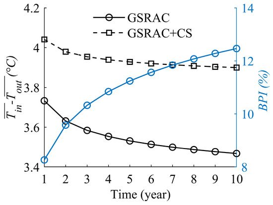
Figure 10.
Fluid temperature differences at the BHE inlet and outlet for the GSRAC and GSRAC + CS systems in black in the left axis, along with the Borehole Performance Improvement (BPI) in blue in the right axis during each year of a simulation.
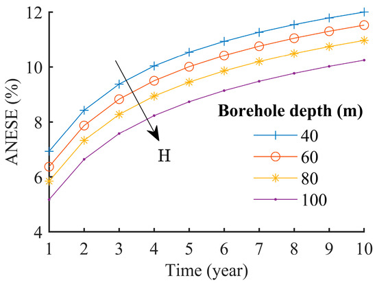
Figure 11.
Variations in annual net energy storage efficiency (ANESE) for different values of BHE depth. The arrow indicates the ascending order of the borehole depth.
5. Parameters Affecting the Performance of GSRAC + CS Systems
In the current study, the four parameters, BHE depth, soil thermal conductivity, spring season duration, and schedule of cold charging and discharging are selected to assess their relative influences on the performance improvement achieved from the addition of CS capability to a conventional GSRAC system.
5.1. The BHE Depth
Figure 11 shows the variations in the ANESE for different values of the BHE depth. The reference simulation is presented for a BHE depth of 80 m. Simulations are also completed for the following BHE depth: 40 m, 60, and 100 m. Although the maximum temperature with a 40 m BHE is much higher than for 100 m, which gives appropriate fluid temperatures, the effect of the thermal rejection is higher in the case of a shallow BHE. This can be explained by the fact that a higher amount of cold energy is expected to dissipate from a larger surface area; therefore, the rate of cold loss is higher for deeper BHEs. Analysis of annual thermal injection of the GSRAC and GSRAC + CS systems indicates that the thermal injection of the conventional system for the 40 m BHE reduces by 7% over ten years, while that for the GSRAC + CS system reduces only by 2.5%, implying that the GSRAC + CS system can work efficiently for a long-term operation. Thus, the effect of integrating TDT into the GSRAC system is to reduce the impact of the soil thermal imbalance problem.
Table 3 presents the average of annual injected energy (into the soil in summer, termed as heat discharged, Qd) and rejected energy (from soil to ambient through heat pipes in winer, termed as head charged, Qc) over the ten years (GWh/year), achieved from the systems with and without heat rejection as well as the average energy storage efficiency, BPI, and the required number of heat pipes to reject the accumulated heat underground for different values of BHE depth.
Table 3.
The annual average injected and rejected energy, average ANESE, and BPI for different borehole depth over ten years, along with the required number of heat pipe modules to reject the accumulated heat underground when the entering water temperature to the BHE during charging and discharging are 11 °C and 40 °C, respectively.
Table 3 reveals that the enhancement in discharged energy due to the “cold” energy charging ( increased with increasing BHE depth because the contact heat transfer area of the BHE and the soil increases. However, a deep BHE demonstrated a lower average ANESE, since the energy dissipation increases with increasing contact heat transfer area.
The BPI decreases with increasing the BHE depth, since the performance deterioration caused by soil thermal imbalance problem is reduced by increasing the BHE depth; therefore, the enhancement in performance of the BHE due to cold energy charging (BPI) is lower for a deep BHE than a shallow one.
Also, from these data, one can calculate the required BHE depth with the heat rejection to achieve the equivalent injected heat without the heat rejection. For example, it is found that to achieve 28.96 GWh heat injection during the warm season by the system with heat rejection, 90 m BHE depth is required. Thus, integrating TDT into the GSRAC system enables the reduction in BHE depth of approximately 10%, thereby reducing the cost of system installation.
5.2. Soil Thermal Conductivity
Figure 12 shows the variations in the ANESE for different values of the soil thermal conductivity. The reference simulation was for a soil thermal conductivity of 1.5 W/(m K). Simulations correspond to the following values of soil thermal conductivity: 1 W/(m K), 2 W/(m K), and 2.5 W/(m K). The high thermal conductivity of the ground leads to an improving heat transfer rate between the ground and the BHE, although it causes more cold accumulation near the BHE, which results in decreasing the ANESE. These results suggest that locations with a lower thermal conductivity of the ground are more appropriate for the installation of BTES systems.
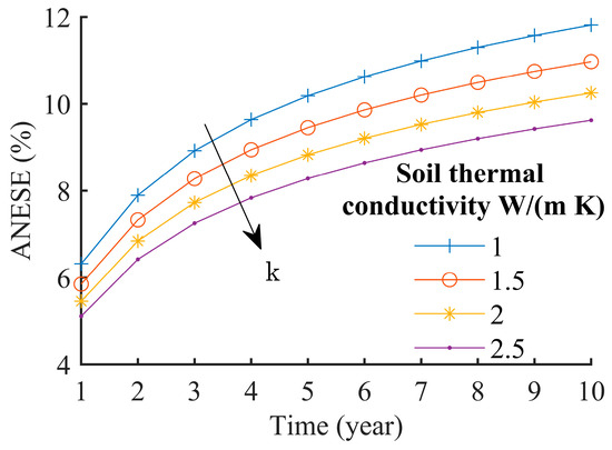
Figure 12.
Variations in annual net energy storage efficiency (ANESE) for different values of soil thermal conductivity. The arrow indicates the ascending order of soil thermal conductivity.
Table 4 presents the average of the annual injected energy (into the soil in summer, termed as heat discharged, Qd) and rejected energy (from soil to ambient through heat pipes in winer, termed as head charged, Qc) over the ten years (GWh/year), achieved from systems with and without heat rejection as well as the average ANESE, BPI, and the required number of heat pipes to reject the accumulated heat underground for different values of soil thermal conductivity. As can be seen from Table 4, as the soil thermal conductivity increases, the enhancement in discharged energy due to the “cold” energy charging ( increases, while the average ANESE and BPI decrease.
Table 4.
The annual average injected and rejected energy, average ANESE, and BPI for different values of thermal conductivity over ten years, along with the required number of heat pipe modules to reject the accumulated heat underground when the entering water temperature to the BHE during charging and discharging are 11 °C and 40 °C, respectively.
From these data, one can also calculate the equivalent thermal conductivity of the ground for a GSRAC + CS to achieve the same performance of a GSRAC system in a better thermal conductivity area. For example, it is found that the performance of GSRAC + CS in an area where the soil thermal conductivity was 2 W/(m K) would be the same as that of a GSRAC in an area where the soil thermal conductivity was 1.85 W/(m K) due to the heat rejection of 15.34 GWh during winter. Thus, the effect of integrating the TDT into the GSRAC system is to compensate for the low thermal conductivity of the ground to some degree.
5.3. Spring Duration
Figure 13 presents the variation in the ANESE for different durations of the spring season, i.e., time intervals between charging and discharging seasons. The reference simulation was for the charging season from June to August and the discharging period from December to February, which represents the spring duration of 3 months, from September to November. Simulations correspond to the following input data:
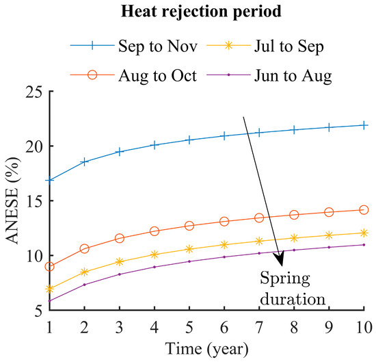
Figure 13.
Variations in annual energy storage efficiency (ANESE) for different durations of spring. The arrow indicates the ascending order of spring duration.
- 0 months (no spring season): charging period from September to November (91 days);
- 1 month: charging period from August to October (92 days);
- 2 months: charging period from July to September (92 days);
- 3 months: charging period from June to August (92 days).
As illustrated in Figure 14, the ANESE increases by reducing the time interval between the charging and discharging seasons (location with no or a short spring season). This can be explained by the fact that the heat accumulated around the BHEs is aggravated when the spring season is longer; therefore, the heat transfer performance and ANESE would deteriorate. Thus, shortening the time interval between the charging and discharging period is beneficial for borehole energy storage systems.
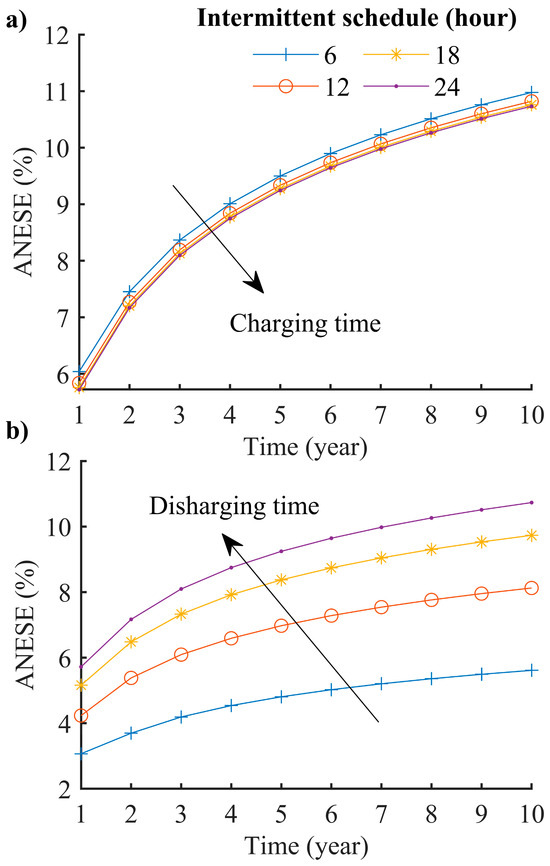
Figure 14.
Variations in annual net energy storage efficiency (ANESE) for different intermittent operations of (a) charging and (b) discharging. The arrows indicate the ascending order of the charging and discharging hours.
Table 5 presents the average of annual injected and rejected energy over the ten years (GWh/year), achieved from the systems with and without heat rejection as well as the average ANESE, BPI, and the required number of heat pipes to reject the accumulated heat underground for different intervals between the charging and discharging periods. Because the spring season duration affects only the GSRAC + CS system, the injected heat for the system without heat rejection is similar for all simulation conditions.
Table 5.
The annual average injected and rejected energy, average ANESE, and BPI for different durations of the spring season over ten years, along with the required number of heat pipe modules to reject the accumulated heat underground when the entering water temperature to the BHE during charging and discharging are 11 °C and 40 °C, respectively.
As it can be seen from Table 5, the injected thermal energy in the case of no spring is much higher than that of a 3-month interval, since there are smaller amounts of energy losses from the storage in case of a no-spring season. Therefore, the enhancement in discharged energy due to the “cold” energy charging ( is maximum in the no-spring case. The increase in spring duration increases the migration rate of cold energy to a far distance from a BHE, thereby reducing the average ANESE and BPI.
5.4. Intermittent Operation for Charging and Discharging Seasons
Figure 14 shows the variation in ANESE for different intermittent operations of charging and discharging. The reference simulation is completed for charging and discharging operations over 24 h. Simulations were run for intermittent operation of 6, 12, 18, and 24 h for charging and discharging operations in such a way that only one of the charging or discharging schedules is changed at any one instance. The intermittent operation of GSRAC can allow for the soil temperature to recover, but the intermittent operation of TDT leads to reducing non-operational hours for soil charging. As can be seen from Figure 14a, the ANESE increases by applying intermittent operation for TDT. This is because the continuous cold charging leads to aggravating thermal energy at a relatively far distance from the BHE and, in the absence of neighbouring boreholes, discharging this aggravated energy is not expected to be possible. However, a reduction in the operating time for the GSRAC system results in reducing the ANESE, as illustrated in Figure 14b. This is due to the fact that the heat injection hours are not long enough to make use of the charged energy in winter; therefore, the aggravated energy near the BHE is much higher than that when the GSRAC system works for 24 h.
Table 6 presents the average of the annual injected and rejected energy over the ten years (GWh/year), achieved from the systems with and without heat rejection as well as the average ANESE, BPI, and the required number of heat pipes to reject the accumulated heat underground for different intermittent operations for charging and discharging. Table 6 suggests that as the daily charging hours increases from 6 to 24 h, the enhancement in discharging energy increases from 0.65 to 1.24 GWh/season, and the average ANESE decreases from 9.27% to 9.03%. However, the BPI increases from 8.48% to 11.1%. Similarly, when the daily discharging operation hours increases from 6 to 24 h, the discharging energy is improved from 0.6 to 1.24 GWh/season, while the average ANESE and BPI increase from 4.7% and 7.73% to 9.03% and 11.1%, respectively.
Table 6.
The annual average injected and rejected energy, average ANESE, and BPI for different intermittent operations of charging and discharging over ten years, along with the required number of heat pipe modules to reject the accumulated heat underground when the entering water temperature to the BHE during charging and discharging are 11 °C and 40 °C, respectively.
As can be seen the injected thermal energy in the case of 6 h charging time was very similar to that of 24 h charging time, implying that a significant amount of charged energy is accumulated near the BHE in the case of the 24 h charging time. Thus, it would be beneficial to select the intermittent operation during charging seasons.
Moreover, the net injected heat in the case of the 24 h discharging time without heat rejection was approximately 23.77 GWh/season, with an average hourly value of 11,005 kWh. This case is comparable to that of the 21 h discharging time with heat rejection, which had an average annual injected heat of approximately 23.77 GWh/season with an average hourly value of 12,576 kWh. Thus, the effect of integrating TDT into the GSRAC system is to reduce the working hours of the RAC unit by 3 h.
Furthermore, one can calculate the energy storage efficiency using the average charged and discharged energy instead of using the net value. The former would be comparable to the calculated ANESE using the net value obtained from the case with a similar intermittent operation for both charging and discharging, for example, a 6 h internment operation for both charging and discharging. It is found that applying intermittent operation for both charging and discharging seasons enhances the ANESE from approximately 9% to 18%, implying that the heat rejection (forced recovery) is more efficient when coupled with natural recovery rather than alone. This is because the rate of accumulated energy near BHE decreases when the soil temperature is close to its undisturbed condition, therefore the ANESE enhances. Thus, it can be concluded that selecting intermittent operation for both charging and discharging periods would generally result in increasing the ANESE.
6. Conclusions
The aim of this paper was to introduce the novel concept of the GSRAC + CS system and demonstrate the performance improvement, which can be achieved from the utilisation of a TDT in the GSRAC system. To limit the impact of soil thermal imbalance, the GSRAC system is coupled with a TDT to collect the “cold” energy from ambient air and store it in the underground soil. In a region with cold winters and hot summers, the TDT can harvest seasonal cold energy and use it to reject the accumulated heat around BHEs to maintain the ground in thermal equilibrium. It was also demonstrated that the TDT improves the efficiency of the GSRAC system in summer. The integration of TDT into the GSRAC system can allow for the utilisation of the GSRAC system in various cooling-dominant applications, such as cooling loads for data centres and food processing plants.
In this study, the soil temperature profiles of systems with and without CS capability were simulated and compared for a ten-year simulation period. It was demonstrated that the soil temperature in the system with CS capability is much lower than that without CS capability. It was also shown that the maximum temperature difference between the two systems occurred at around 2–3 m and 0.3 m from the BHE wall and bottom end of the borehole, respectively.
The main outcomes of the case study indicate the following:
- The integration of TDT into the GSRAC system can not only help to reduce the impact of soil thermal imbalance and the required BHE depth, but can also help to compensate for the low thermal conductivity of the ground and reduce the operational time of the RAC unit;
- In comparison with the GSRAC system, the GSRAC + CS system requires 10% less BHE depth to achieve a similar amount of heat injected into the ground;
- A comparison between the fluid temperatures at the inlet and outlet of the two systems revealed that the seasonal energy storage can improve the overall performance of a single BHE on average by 11%;
- The accumulated energy near a BHE is the most critical factor influencing the ANESE while using a single BHE thermal energy storage system;
- The shallower BHEs demonstrated slightly better ANESE and BPI, but a higher amount of energy can be discharged from deeper BHEs;
- To achieve better performance and reduce accumulated energy in the storage region, the time interval between charging and discharging periods should be set to a minimum value;
- To maximise the ANESE of a single BHE and reduce the accumulated energy near a BHE, it would be beneficial to select an intermittent operation for both charging and discharging seasons.
As mentioned earlier, the primary aim of the current study was to introduce the GSRAC + CS system concept; therefore, further research is needed to confirm the theoretically obtained effects and dependencies. For example, a small-scale demonstration rig would provide a better understanding of the feasibility and efficiency of the GSRAC + CS system. Further research can also be focused on the study of the factors affecting the performance of TDT, for instance, a sensitivity study on the changing ambient weather conditions and the capacity of TDT and their effects on the performance of the GSRAC system. Further research might also explore the possible integration of TDT into a GSRAC system with multiple BHEs. By increasing the number of BHEs, the thermal energy stored by each BHE can be discharged by adjacent BHEs. Therefore, the aggravated thermal energy in the soil would reduce and the ANESE and BPI would increase.
Author Contributions
Conceptualization, E.H.; Methodology, E.H.; Formal analysis, A.D.; Investigation, A.D.; Writing—original draft, A.D.; Writing—review & editing, E.H.; Supervision, E.H. and A.K. All authors have read and agreed to the published version of the manuscript.
Funding
This research received no external funding.
Data Availability Statement
The original contributions presented in this study are included in the article. Further inquiries can be directed to the corresponding author.
Acknowledgments
We would like to acknowledge the support provided by the School of Mechanical Engineering at The University of Adelaide, Australia. The first-named author has received an Adelaide Graduate Research Scholarship. This work was supported with supercomputing resources provided by the Phoenix HPC service at The University of Adelaide.
Conflicts of Interest
The authors declare no conflict of interest.
Abbreviations
| Nomenclature | Greek Symbols | ||
| Area of the heat pipe [m2] | [K] | ||
| Thermal capacity of the fluid [J/(K kg)] | Subscripts | ||
| End time of charging period | ambient | ||
| End time of discharging period | Condenser section of the heat pipe | ||
| Borehole depth [m] | Evaporator section of the heat pipe | ||
| Heat transfer coefficient | inner | ||
| Thermal conductivity [W/(m K)] | outer | ||
| Length of heat pipe [m] | v | Vapour inside the heat pipe | |
| Number of heat pipes | w | Water inside the TDT | |
| Heat injection into the soil during discharging period [Wh/year] | Abbreviations | ||
| Heat injection into the soil during discharging period [Wh/year] | ANESE | Annual Net Energy Storage Efficiency | |
| Heat extraction from the soil during charging period [Wh/year] | BHEs | Borehole Heat Exchanger(s) | |
| Heat extraction from the soil [W] | BMP | Borehole field MATLAB-based Programme | |
| Heat dissipation from the TDT [W] | BPI | Borehole Performance Improvement | |
| Thermalfrom days 184 to 273 resistance [(m K)/W] | Borehole Thermal Energy Storage | ||
| Convective thermal resistance [(m K)/W] | FDM | Finite Difference Method | |
| Radiative thermal resistance [(m K)/W] | TDT | Thermal Diode Tank | |
| Half shank spacing [m] | GSRAC | Ground Source Refrigeration and Air-Conditioning | |
| Start time of charging period | CS | Cold energy Storage | |
| Start time of discharging period | RAC | Refrigeration and Air Conditioning | |
Appendix A. The Thermal Diode Tank (TDT) Model
This appendix describes the TDT model. This model is developed to find the required numbers of heat pipes to achieve a certain temperature difference between the water inside the tank and the ambient air (). Therefore, the fluid temperature inside the TDT is estimated based on the energy balance equation under steady-state conditions. The model is based on two assumptions:
- The axial conduction in the fluid is negligible;
- Heat losses from the TDT wall to the ambient are negligible.
The energy balance can be written as follows:
In the above equation, denotes the extracted heat from the soil, denotes the heat dissipation from the TDT to the ambient air using the thermosyphon heat pipe, and is the number of thermosyphon heat pipes inside the water tank. When the BHE is connected to the TDT unit, the value of can be found as follows:
where is the flow rate of the upcoming fluid from the BHE, is the specific heat capacity of the upcoming fluid from the BHE, is the outlet water temperature from the BHE to TDT, and is the inlet fluid temperature to the BHE from the TDT, which is assumed to be equal to the mean water temperature inside the TDT. The value of can be found using the thermal resistance terminology, as shown in Figure A1.

Figure A1.
Thermal resistance diagram of the TDT.
In the above figure, is the ambient air temperature; is the temperature of the outer surface of the condenser wall, is the temperature of the inner surface of the condenser wall, is the vapour temperature of the refrigerant inside the thermosyphon heat pipe, is the temperature of the inner surface of the evaporator wall, is the temperature of the outer surface of the evaporator wall, is the mean water temperature inside the tank that is equal to in charging operation, and is the heat extraction rate from the soil in charging seasons. The equations for thermal resistances are listed in Table A1.
Table A1.
Thermal resistance equations.
Table A1.
Thermal resistance equations.
| R | Description | Equation | |
|---|---|---|---|
| The convective-radiative resistance from the outer surface of the condenser to the ambient air | (A3) | ||
| The conductive resistance between the outer and inner surfaces of the condenser | (A4) | ||
| The convective resistance between the vapour and inner surface of the condenser | (A5) | ||
| The convective resistance between the vapour and the inner surface of the evaporator | (A6) | ||
| The conductive resistance between the outer and inner surface of the evaporator | (A7) | ||
| The convective resistance from the outer surface of the evaporator to the water | (A8) |
Therefore, can be written as follows:
Based on the assumption that the required temperature difference between the water temperature inside the tank and the ambient air temperature is , the following can be written:
Substituting Equations (A3) and (A8) to (A1) leads to the following:
Substituting Equation (A10) into the above equation, leads to the following:
Finally, solving the above equation for the required number of the heat pipe modules leads to the following:
References
- Zhang, H.; Shao, S.; Xu, H.; Zou, H.; Tang, M.; Tian, C. Numerical investigation on integrated system of mechanical refrigeration and thermosyphon for free cooling of data centers. Int. J. Refrig. 2015, 60, 9–18. [Google Scholar] [CrossRef]
- Santos, A.F.; Gaspar, P.D.; de Souza, H.J. Refrigeration of COVID-19 Vaccines: Ideal Storage Characteristics, Energy Efficiency and Environmental Impacts of Various Vaccine Options. Energies 2021, 14, 1849. [Google Scholar] [CrossRef]
- Cansino, J.M.; Pablo-Romero, M.d.P.; Román, R.; Yñiguez, R. Promoting renewable energy sources for heating and cooling in EU-27 countries. Energy Policy 2011, 39, 3803–3812. [Google Scholar] [CrossRef]
- Yan, C.; Shi, W.; Li, X.; Wang, S. A seasonal cold storage system based on separate type heat pipe for sustainable building cooling. Renew. Energy 2016, 85, 880–889. [Google Scholar] [CrossRef]
- Li, G.; Hwang, Y.; Radermacher, R. Review of cold storage materials for air conditioning application. Int. J. Refrig. 2012, 35, 2053–2077. [Google Scholar] [CrossRef]
- IRENA. Innovation Outlook: Thermal Energy Storage; International Renewable Energy Agency Abu Dhabi: Abu Dhabi, United Arab Emirates, 2020. [Google Scholar]
- Fleuchaus, P.; Godschalk, B.; Stober, I.; Blum, P. Worldwide application of aquifer thermal energy storage—A review. Renew. Sustain. Energy Rev. 2018, 94, 861–876. [Google Scholar] [CrossRef]
- Brown, D.R. Thermal Energy for Space Cooling-Federal Technology Alert; Pacific Northwest National Lab: Richland, WA, USA, 2000. [Google Scholar]
- Abbas, Z.; Chen, D.; Li, Y.; Yong, L.; Wang, R.Z. Experimental investigation of underground seasonal cold energy storage using borehole heat exchangers based on laboratory scale sandbox. Geothermics 2020, 87, 101837. [Google Scholar] [CrossRef]
- Kharseh, M.; Al-Khawaja, M.; Suleiman, M.T. Potential of ground source heat pump systems in cooling-dominated environments: Residential buildings. Geothermics 2015, 57, 104–110. [Google Scholar] [CrossRef]
- Hwang, Y.; Lee, J.K.; Jeong, Y.M.; Koo, K.M.; Lee, D.H.; Kim, I.K.; Jin, S.W.; Kim, S.H. Cooling performance of a vertical ground-coupled heat pump system installed in a school building. Renew. Energy 2009, 34, 578–582. [Google Scholar] [CrossRef]
- You, T.; Wu, W.; Shi, W.; Wang, B.; Li, X. An overview of the problems and solutions of soil thermal imbalance of ground-coupled heat pumps in cold regions. Appl. Energy 2016, 177, 515–536. [Google Scholar] [CrossRef]
- Zhao, Z.; Shen, R.; Feng, W.; Zhang, Y.; Zhang, Y. Soil thermal balance analysis for a ground source heat pump system in a hot-summer and cold-winter region. Energies 2018, 11, 1206. [Google Scholar] [CrossRef]
- Bayer, P.; de Paly, M.; Beck, M. Strategic optimization of borehole heat exchanger field for seasonal geothermal heating and cooling. Appl. Energy 2014, 136, 445–453. [Google Scholar] [CrossRef]
- Wu, W.; You, T.; Wang, B.; Shi, W.; Li, X. Simulation of a combined heating, cooling and domestic hot water system based on ground source absorption heat pump. Appl. Energy 2014, 126, 113–122. [Google Scholar] [CrossRef]
- Emmi, G.; Zarrella, A.; De Carli, M.; Donà, M.; Galgaro, A. Energy performance and cost analysis of some borehole heat exchanger configurations with different heat-carrier fluids in mild climates. Geothermics 2017, 65, 158–169. [Google Scholar] [CrossRef]
- Fang, H.; Xia, J.; Lu, A.; Jiang, Y. An operation strategy for using a ground heat exchanger system for industrial waste heat storage and extraction. Build. Simul. 2014, 7, 197–204. [Google Scholar] [CrossRef]
- Ni, L.; Song, W.; Zeng, F.; Yao, Y. Energy Saving and Economic Analyses of Design Heating Load Ratio of Ground Source Heat Pump with Gas Boiler as Auxiliary Heat Source. In Proceedings of the 2011 International Conference on Electric Technology and Civil Engineering (ICETCE), Lushan, China, 22–24 April 2011; pp. 1197–1200. [Google Scholar] [CrossRef]
- Naranjo-Mendoza, C.; Oyinlola, M.A.; Wright, A.J.; Greenough, R.M. Experimental study of a domestic solar-assisted ground source heat pump with seasonal underground thermal energy storage through shallow boreholes. Appl. Therm. Eng. 2019, 162, 114218. [Google Scholar] [CrossRef]
- You, T.; Wang, B.; Wu, W.; Shi, W.; Li, X. A new solution for underground thermal imbalance of ground-coupled heat pump systems in cold regions: Heat compensation unit with thermosyphon. Appl. Therm. Eng. 2014, 64, 283–292. [Google Scholar] [CrossRef]
- Rees, S. Advances in Ground-Source Heat Pump Systems; Woodhead Publishing: Amsterdam, The Netherlands, 2016. [Google Scholar]
- Sun, Y.; Guan, Z.; Hooman, K. A review on the performance evaluation of natural draft dry cooling towers and possible improvements via inlet air spray cooling. Renew. Sustain. Energy Rev. 2017, 79, 618–637. [Google Scholar] [CrossRef]
- Wang, X.; Bierwirth, A.; Christ, A.; Whittaker, P.; Regenauer-Lieb, K.; Chua, H.T. Application of geothermal absorption air-conditioning system: A case study. Appl. Therm. Eng. 2013, 50, 71–80. [Google Scholar] [CrossRef]
- Lanahan, M.; Tabares-Velasco, P.C. Seasonal thermal-energy storage: A critical review on BTES systems, modeling, and system design for higher system efficiency. Energies 2017, 10, 743. [Google Scholar] [CrossRef]
- Singh, R.; Mochizuki, M.; Mashiko, K.; Nguyen, T. Heat pipe based cold energy storage systems for datacenter energy conservation. Energy 2011, 36, 2802–2811. [Google Scholar] [CrossRef]
- Delazar, A.; Hu, E.; Kotousov, A.; Sofyan, S.E. A novel three-dimensional implicit numerical model of a borehole field heat exchanger that accounts for seasonal fluctuations of the soil temperature. Geothermics 2021, 97, 102236. [Google Scholar] [CrossRef]
- Sofyan, S.E.; Hu, E.; Kotousov, A.; Riayatsyah, T.M.I. A new approach to modelling of seasonal soil temperature fluctuations and their impact on the performance of a shallow borehole heat exchanger. Case Stud. Therm. Eng. 2020, 22, 100781. [Google Scholar] [CrossRef]
- Lu, Q.; Narsilio, G.A.; Aditya, G.R.; Johnston, I.W. Economic analysis of vertical ground source heat pump systems in Melbourne. Energy 2017, 125, 107–117. [Google Scholar] [CrossRef]
- Remeli, M.F.; Tan, L.; Date, A.; Singh, B.; Akbarzadeh, A. Simultaneous power generation and heat recovery using a heat pipe assisted thermoelectric generator system. Energy Convers. Manag. 2015, 91, 110–119. [Google Scholar] [CrossRef]
- Bureau of Meteorology. Greater Adelaide in Winter 2021. Available online: http://www.bom.gov.au/climate/current/season/sa/adelaide.shtml (accessed on 17 November 2021).
- Eskilson, P. Thermal Analysis of Heat Extraction Boreholes. Ph. D. Thesis, University of Lund, Lund, Sweden, 1987. [Google Scholar]
- Catolico, N.; Ge, S.; McCartney, J.S. Numerical Modeling of a Soil-Borehole Thermal Energy Storage System. Vadose Zone J. 2016, 15, 1–17. [Google Scholar] [CrossRef]
- Wołoszyn, J. Global sensitivity analysis of borehole thermal energy storage efficiency on the heat exchanger arrangement. Energy Convers. Manag. 2018, 166, 106–119. [Google Scholar] [CrossRef]
Disclaimer/Publisher’s Note: The statements, opinions and data contained in all publications are solely those of the individual author(s) and contributor(s) and not of MDPI and/or the editor(s). MDPI and/or the editor(s) disclaim responsibility for any injury to people or property resulting from any ideas, methods, instructions or products referred to in the content. |
© 2025 by the authors. Licensee MDPI, Basel, Switzerland. This article is an open access article distributed under the terms and conditions of the Creative Commons Attribution (CC BY) license (https://creativecommons.org/licenses/by/4.0/).